Ultraslow Helical Optical Bullets and Their Acceleration in Magneto-Optically Controlled Coherent Atomic Media

Abstract

We propose a scheme to produce ultraslow (3+1)-dimensional helical optical solitons, alias helical optical bullets, in a resonant three-level $\Lambda$-type atomic system via quantum coherence. We show that, due to the effect of electromagnetically induced transparency, the helical optical bullets can propagate with an ultraslow velocity up to $10^{-5}$ $c$ ($c$ is the light speed in vacuum) in longitudinal direction and a slow rotational motion (with velocity $10^{-7}$ $c$) in transverse directions. The generation power of such optical bullets can be lowered to microwatt, and their stability can be achieved by using a Bessel optical lattice potential formed by a far-detuned laser field. We also show that the transverse rotational motion of the optical bullets can be accelerated by applying a time-dependent Stern-Gerlach magnetic field. Because of the untraslow velocity in the longitudinal direction, a significant acceleration of the rotational motion of optical bullets may be observed for a very short medium length.

I Introduction

In recent years, the formation and propagation of a new type of optical solitons, i.e. ultraslow optical solitons, created in resonant multi-level media via electromagnetically induced transparency (EIT) fle , has attracted much attention wu ; huang ; hang1 ; yang . By the quantum interference effect induced by a control field, the absorption of a probe field can be largely suppressed. Simultaneously, a drastic change of dispersion and a giant enhancement of Kerr nonlinearity can be achieved via EIT. It has been shown that, by the balance of the dispersion and the Kerr nonlinearity, temporal optical solitons with very small propagating velocity and very low generation power can form and propagate stably for a long distance. The possibility of producing weak-light spatial and spatia-temporal optical solitons in EIT-based media has also been suggested hong ; hang2 ; MPP ; HK ; LWH .

On the other hand, the optical beam deflection in an atomic system with inhomogeneous external magnetic fields has been the subject of many previous works SW ; hol ; ZZWYS . Physically, atomic energy levels are space-dependent if an inhomogeneous magnetic field is applied, which results in a spatial dependence of optical refraction index of the atomic medium and hence a deflection of optical beam when passing through the medium. In a remarkable experiment KW , Karpa and Weitz demonstrated that photons can acquire effective magnetic moments when propagating in EIT media, and hence can deflect significantly in a transverse gradient magnetic field, which is regarded as an optical analog of Stern-Gerlach (SG) effect of atoms. The work by Karpa and Weitz KW has stimulated a flourished theoretical and experimental studies on the SG effect of slow light via EIT ZLZS ; liy ; GZKS ; KW1 . Recently, a scheme to exhibit EIT-enhanced SG deflection of weak-light vector optical solitons in an EIT medium has been suggested HH .

In this article, we propose a scheme to produce ultraslow (3+1)-dimensional helical optical solitons, alias helical optical bullets, in a resonant three-level $\Lambda$-type atomic system via quantum coherence. We show that due to the EIT effect the helical optical bullets found can propagate with ultraslow velocity up to $10^{-5}$ $c$ ($c$ is the light speed in vacuum) in longitudinal direction and a slow rotational motion (with velocity $10^{-7}$ $c$) in transverse directions. The generation power of such optical bullets can be lowered to the magnitude of microwatt, and their stability can be achieved by using a Bessel optical lattice potential formed by a far-detuned laser field. We also show that the transverse rotational motion of the optical bullets can be accelerated by the use of a time-dependent SG magnetic field. Because of the ultraslow velocity in the longitudinal direction, a significant acceleration of the rotational motion of the optical bullets may be observed for a very short medium length.

We stress that the ultraslow helical optical bullets found here have many attractive features. First, because of the giant Kerr nonlinearity induced by the EIT effect the optical bullets can form in a very short distance (at the order of centimeter) with extremely low generation power (at the order of microwatt). Second, they have ultraslow propagating velocity which prolongs the interaction time between light and atoms. Third, their motional trajectories are helical curves (see Fig. 4(c) below). Fourth, because of the active character of our system it is very easy to realize an efficient magneto-optical manipulation of the helical optical bullets by using the energy-level structure of atoms and selection rules of optical transitions. Due to these features, the ultraslow helical optical bullets obtained here may become candidates for light information processing and transmission at a very weak light level. Note that in recent years several authors have done interesting works on linear and nonlinear matter waves in Bose-Einstein condensates with toroidal traps and realized their acceleration JPY1 ; DJM ; RACN ; BK . However, in those works no ultraslow bullets and their helical motion have been obtained.

Our article is arranged as follows. In Sec. II, the physical model of a three-state atomic system with a $\Lambda$-type energy-level configuration is described. Maxwell-Bloch (MB) equations governing the motion of density matrix elements and the probe-field Rabi frequency are given. In Sec. III, a nonlinear envelope equation governing the motion of the probe-field is derived based on a standard method of multiple-scales. In Sec. IV, the formation and propagation of ultraslow high-dimensional helical optical bullets are discussed. In Sec. V, the stability of helical optical solitons is analyzed and their acceleration is investigated in detail. The last section (Sec. VI) contains a discussion and summary of main results of our work.

II Model

We consider a resonant, lifetime-broadened atomic gas with a $\Lambda$-type energy-level configuration (Fig. 1(a) ), which

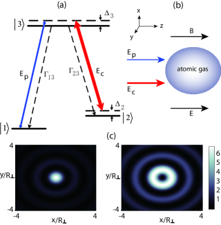
Figure 1: (Color online) (a): Energy-level diagram and excitation scheme of $\Lambda$-type three-level atoms interacting with a weak pulsed probe field $E_{p}$ and a strong CW control field $E_{c}$. $\Delta_{2}$ and $\Delta_{3}$ are the two- and one-photon detunings, respectively. $\Gamma_{13}$ and $\Gamma_{23}$ are the decay rates from $|3\rangle$ to $|1\rangle$ and from $|3\rangle$ to $|2\rangle$, respectively. (b): The coordinate frame used for calculations and geometrical arrangement of the system. The shadow region denotes the atomic gas confined in a cell, $B$ and $E$ are gradient magnetic field and far-detuned laser field, respectively. (c): Left (right) part corresponds to the light-intensity distribution of the zero (first) order Bessel lattice $J_{0}^{2}(2r)$ ($J_{1}^{2}(2r)$ ) in the $(x,y)$ plane, with $r=(x^{2}+y^{2})^{1/2}$ and $R_{\bot}$ the probe beam radius.

interacts with a strong, continuous-wave (CW) control field of angular frequency $\omega_{c}$ that drives the transition $|2\rangle\leftrightarrow|3\rangle$ and a weak, pulsed probe field (with the pulse length $\tau_{0}$ and radius $R_{\bot}$ at the entrance of the medium) of center angular frequency $\omega_{p}$ that drives the transition $|1\rangle\leftrightarrow|3\rangle$, respectively. $\Delta_{2}$ and $\Delta_{3}$ are respectively the two- and one-photon detunings, $\Gamma_{13}$ and $\Gamma_{23}$ are respectively the decay rates from $|3\rangle$ to $|1\rangle$ and from $|3\rangle$ to $|2\rangle$. The electric-field vector of the system can be written as $\mathbf{E}=\mathbf{E}_{p}+\mathbf{E}_{c}=\sum_{l=c,p}{\mathbf{e}_{l}\mathcal{E}}_{l}\exp[i(k_{l}z-\omega_{l}t)]+{\rm c.c}.$, where $\mathbf{e}_{c}$ and $\mathbf{e}_{p}$ ($\mathcal{E}_{c}$ and $\mathcal{E}_{p}$) are respectively the polarization unit vectors (envelopes) of the control and probe fields, $k_{p}=\omega_{p}/c$ and $k_{c}=\omega_{c}/c$ are respectively the center wavenumbers of the probe and control fields. For simplicity, both the probe and the control fields are taken to propagate along $z$-direction.

We assume a weak, time-dependent gradient magnetic field with the form

$${\bf B}(t)=\hat{\bf z}f(t)Bx,$$ (1)

is applied to the system, where $\hat{\bf z}$ is the unit vector in $z$-direction and $B$ characterizes magnitude of the gradient and $f(t)$ describes its time dependence. Due to the presence of ${\bf B}(t)$, Zeeman level shift $\Delta E_{j,\rm Zeeman}=\mu_{B}g_{F}^{j}m_{F}^{j}f(t)Bx$ occurs for all levels. Here $\mu_{B}$, $g_{F}^{j}$, and $m_{F}^{j}$ are Bohr magneton, gyromagnetic factor, and magnetic quantum number of the level $|j\rangle$, respectively. The aim of introducing the SG gradient magnetic field (1) is to produce an external force in transverse directions to control the motion of optical bullets formed by the probe field.

In addition, we assume further a weak, far-detuned laser field with the form

$${\bf E}(r,t)=\hat{\bf z}\,pJ_{l}(\sqrt{2b}r)\cos(\omega_{E}t),$$ (2)

is also applied into the system. Here $r=\sqrt{x^{2}+y^{2}}$, $J_{l}$ is the $l$-order Bessel function with $p$ and $b$ characterizing respectively its amplitude and radius, and $\omega_{E}$ is oscillating angular frequency. Due to the presence of ${\bf E}(r,t)$, Stark level shift $\Delta E_{j,\rm Stark}=-\frac{1}{2}\alpha_{j}\langle E^{2}\rangle_{t}=-\frac{1}{4}\alpha_{j}p^{2}J_{l}^{2}(\sqrt{2b}r)$ occurs for all levels, where $\alpha_{j}$ is the scalar polarizability of the level $|j\rangle$. Shown in the left (right) part of Fig. 1(c) is the light-intensity distribution corresponding to the zero (first) order Bessel lattice $J_{0}^{2}(2r)$ ($J_{1}^{2}(2r)$ ). The aim of introducing the far-detuned laser field (2) is to form a trapping lattice potential in the transverse directions to stabilize the optical bullets. A possible geometrical arrangement of the system is given in Fig. 1(b).

Under electric-dipole and rotating-wave approximations, in interaction picture equations of motion for the density matrix elements are given by

$$i\frac{\partial}{\partial t}\sigma_{11}-i\Gamma_{13}\sigma_{33}+\Omega_{p}^{\ast}\sigma_{31}-\Omega_{p}\sigma_{31}^{\ast}=0,$$ (3a)

$$i\frac{\partial}{\partial t}\sigma_{22}-i\Gamma_{23}\sigma_{33}+\Omega_{c}^{\ast}\sigma_{32}-\Omega_{c}\sigma_{32}^{\ast}=0,$$ (3b)

$$i\frac{\partial}{\partial t}\sigma_{33}+i\Gamma_{3}\sigma_{33}-\Omega_{p}^{\ast}\sigma_{31}+\Omega_{p}\sigma_{31}^{\ast}-\Omega_{c}^{\ast}\sigma_{32}+\Omega_{c}\sigma_{32}^{\ast}=0,$$ (3c)

$$\left(i\frac{\partial}{\partial t}+d_{21}\right)\sigma_{21}-\Omega_{p}\sigma_{32}^{\ast}+\Omega_{c}^{\ast}\sigma_{31}=0,$$ (3d)

$$\left(i\frac{\partial}{\partial t}+d_{31}\right)\sigma_{31}-\Omega_{p}(\sigma_{33}-\sigma_{11})+\Omega_{c}\sigma_{21}=0,$$ (3e)

$$\left(i\frac{\partial}{\partial t}+d_{32}\right)\sigma_{32}-\Omega_{c}(\sigma_{33}-\sigma_{22})+\Omega_{p}\sigma_{21}^{\ast}=0,$$ (3f)

where $\Omega_{p}=\mathbf{e}_{p}\cdot\mathbf{p}_{31}\mathcal{E}_{p}/\hbar$ and $\Omega_{c}=\mathbf{e}_{c}\cdot\mathbf{p}_{32}\mathcal{E}_{c}/\hbar$ are respectively the half Rabi frequencies of the probe and the control fields, with $\mathbf{p}_{jl}$ being the electric dipole matrix element associated with the transition from $|l\rangle$ to $|j\rangle$. In Eq. (3), we have defined $d_{21}=\Delta_{2}+i\gamma_{21}$, $d_{31}=\Delta_{3}+i\gamma_{31}$, and $d_{32}=(\Delta_{3}-\Delta_{2})+i\gamma_{32}$, where $\Delta_{2}$ and $\Delta_{3}$ are two- and one-photon detunings given respectively by $\Delta_{2}=\delta_{2}+\mu_{21}f(t)Bx-\frac{1}{4}\alpha_{21}p^{2}J_{l}^{2}(\sqrt{2b}r)$ and $\Delta_{3}=\delta_{3}+\mu_{31}f(t)Bx-\frac{1}{4}\alpha_{31}p^{2}J_{l}^{2}(\sqrt{2b}r)$, with $\mu_{jl}=\mu_{B}(g_{F}^{j}m_{F}^{j}-g_{F}^{l}m_{F}^{l})/\hbar$ and $\alpha_{jl}=(\alpha_{j}-\alpha_{l})/\hbar$. Here $\delta_{2}=\omega_{p}-\omega_{c}-\omega_{21}$ and $\delta_{3}=\omega_{p}-\omega_{31}$, where $\omega_{jl}=(E_{j}-E_{l})/\hbar$ with $E_{j}$ being the eigenenergy of the state $|j\rangle$. $\gamma_{jl}=(\Gamma_{j}+\Gamma_{l})/2+\gamma_{jl}^{\rm col}$, where $\Gamma_{j}=\sum_{j<l}\Gamma_{jl}$ with $\Gamma_{jl}$ being the spontaneous emission decay rate from $|l\rangle$ to $|j\rangle$ and $\gamma_{jl}^{\rm col}$ being the dephasing rate reflecting the loss of phase coherence between $|j\rangle$ and $|l\rangle$ without changing of population, as might occur by elastic collisions.

The equation of motion for $\Omega_{p}(x,y,z,t)$ can be obtained by the Maxwell equation, which under slowly-varying envelope approximation reads

$$i\left(\frac{\partial}{\partial z}+\frac{1}{c}\frac{\partial}{\partial t}\right)\Omega_{p}+\frac{c}{2\omega_{p}}\left(\frac{\partial^{2}}{\partial x^{2}}+\frac{\partial^{2}}{\partial x^{2}}\right)\Omega_{p}+\kappa_{13}\sigma_{31}=0,$$ (4)

where $\kappa_{13}=N_{a}\omega_{p}|\mathbf{p}_{13}|^{2}/(2\varepsilon_{0}c\hbar)$ with $N_{a}$ being the atomic concentration.

Our model can be easily realized by experiment. One of candidates is the cold ⁸⁵Rb atomic gas with the energy-levels in Fig. 1(a) assigned as $|1\rangle=|5^{2}S_{1/2},F=2\rangle$, $|2\rangle=|5^{2}S_{1/2},F=3\rangle$, and $|3\rangle=|5^{2}P_{1/2},F=2\rangle$. Then, the decay rates in the Bloch Eq. (3) are given by $\Gamma_{13}\approx\Gamma_{23}=5.9$ MHz and $\gamma_{13}^{\rm col}\approx\gamma_{23}^{\rm col}=50$ Hz. In addition, we take $N_{a}=10^{12}$ cm^-3, then $\kappa_{13}$ in the Maxwell Eq. (4) takes the value $1.0\times 10^{9}$ cm^-1s^-1. We shall use these system parameters in the following calculations.

III (3+1)-dimensinal nonlinear envelope equation

The base state solution (i.e. the steady-state solution for vanishing $\Omega_{p}$) of the MB Eqs. (3) and (4) is $\sigma_{11}=1$ and other $\sigma_{jl}$ are zero. When a weak probe field (i.e. $\Omega_{p}$ is very small) is applied, the system undergoes a linear evolution. In this case, the MB Eqs. (3) and (4) can be linearized with the solution given by

$$\Omega_{p}=Ae^{i[K(\omega)z-\omega t]},$$ (5a)

$$\sigma_{j1}=\frac{\delta_{j3}(\omega+\delta_{2}+i\gamma_{21})-\delta_{j2}\Omega_{c}^{\ast}}{D(\omega)}Ae^{i(K(\omega)z-\omega t)},\quad(j=2,3)$$ (5b)

together with $\sigma_{jj}=\delta_{j1}$ and $\sigma_{32}=0$. Here $A$ is a constant, $\delta_{jk}$ is Kronecker delta symbol, and $K(\omega)$ is the linear dispersion relation of the system

$$K(\omega)=\frac{\omega}{c}+\kappa_{13}\frac{\omega+\delta_{2}+i\gamma_{21}}{D(\omega)}$$ (6)

with $D(\omega)=|\Omega_{c}|^{2}-(\omega+\delta_{2}+i\gamma_{21})(\omega+\delta_{3}+i\gamma_{31})$. Here $\omega$ and $K(\omega)$ are respectively the deviations of the frequency and wavenumber of the probe field note1 . In obtaining Eq. (6) we have neglected the transverse diffraction effect which is usually negligible in the leading order approximation of Eq. (4). For illustration, in the panels (a)

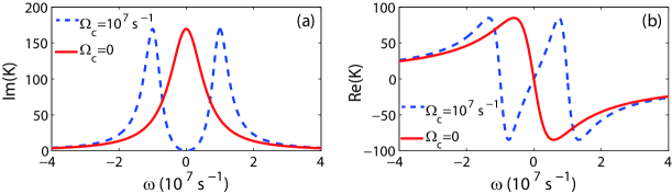
Figure 2: (Color online) Im$(K)$ (a) and Re$(K)$ (b) as functions of $\omega$. The dashed and solid lines in each panel correspond to the presence ($\Omega_{c}=1.0\times 10^{7}$ ${\rm s}^{-1}$) and the absence ($\Omega_{c}=0$) of the control field, respectively.

and (b) of Fig. 2 we have plotted the real part Re$(K)$ and the imaginary part Im$(K)$ as a function of $\omega$ for $\Delta_{2}=\Delta_{3}=0$. The dashed and solid lines in the figure correspond respectively to the absence ($\Omega_{c}=0$) and the presence ($\Omega_{c}=1.0\times 10^{7}$ ${\rm s}^{-1}$) of the control field. One sees that when $\Omega_{c}=0$, the probe field has a large absorption (the solid line of panel (a) ); however, when $\Omega_{c}\neq 0$ and increases to a large value, a transparency window is opened in the probe-field absorption spectrum (the dashed line of panel (a) ), and hence the probe field can propagate in the resonant atomic system with negligible absorption, a basic character of EIT. On the other hand, for the large control field the slope of Re$(K)$ is drastically changed and steepened (see the dashed line of panel (b) ) which results in a significant reduction of the group velocity of the probe field (and hence slow light). All these interesting characters are due to the quantum interference effect induced by the control field fle .

However, although the absorption is largely suppressed by the EIT effect, the probe pulse may still suffers a serious distortion during propagation because of the existence of the dispersion and diffraction. To avoid such distortion and obtain a long-distance propagation of shape-preserving probe pulses, a natural idea is to use nonlinear effect to balance the dispersion and diffraction. One of important shape-preserving (3+1)-dimensional probe pulses is optical bullet.

For this aim, we first derive a (3+1)-dimensional nonlinear envelope equation that includes the dispersion, diffraction, and nonlinearity of the system. We take the asymptotic expansion

$$\sigma_{jk}=\sigma_{jk}^{(0)}+\epsilon\sigma_{jk}^{(1)}+\epsilon^{2}\sigma_{jk}^{(2)}+\epsilon^{3}\sigma_{jk}^{(3)}+\cdots,\quad(j,\,k=1,\,2,\,3),$$ (7a)

$$\Omega_{p}=\epsilon\Omega_{p}^{(1)}+\epsilon^{2}\Omega_{p}^{(2)}+\epsilon^{3}\Omega_{p}^{(3)}+\cdots,$$ (7b)

$$d_{j1}=d_{j1}^{(0)}+\epsilon d_{j1}^{(1)}+\epsilon^{2}d_{j1}^{(2)}+\cdots,\quad(j=2,\,3),$$ (7c)

$$d_{32}=d_{32}^{(0)}+\epsilon d_{32}^{(1)}+\epsilon^{2}d_{32}^{(2)}+\cdots,$$ (7d)

with $\sigma_{jk}^{(0)}=\delta_{j1}\delta_{k1}$. Additionally, we assume both the gradient magnetic field (1) and the far-detuned laser field (2) are of order of $\epsilon$. Thus we have $d_{21}^{(0)}=\delta_{2}+i\gamma_{21}$, $d_{31}^{(0)}=\delta_{3}+i\gamma_{31}$, $d_{32}^{(0)}=\delta_{3}-\delta_{2}+i\gamma_{32}$, $d_{21}^{(1)}=d_{31}^{(1)}=d_{32}^{(1)}=0$, $d_{21}^{(2)}=\mu_{21}f(t_{2})Bx_{1}-\frac{1}{4}\alpha_{21}p^{2}J_{l}^{2}(\sqrt{2b}r_{1})$, $d_{31}^{(2)}=\mu_{31}f(t_{2})Bx_{1}-\frac{1}{4}\alpha_{31}p^{2}J_{l}^{2}(\sqrt{2b}r_{1})$, and $d_{32}^{(2)}=\mu_{32}f(t_{2})Bx_{1}-\frac{1}{4}\alpha_{32}p^{2}J_{l}^{2}(\sqrt{2b}r_{1})$. Here $\epsilon$ is a dimensionless small parameter characterizing the amplitude of the probe field. All quantities on the right hand side of the expansion (7) are considered as functions of the multi-scale variables $z_{l}=\epsilon^{m}z$ ($m=0$ to $2$), $t_{2}=\epsilon^{2}t$, $x_{1}=\epsilon x$, $y_{1}=\epsilon y$, and $r_{1}=\sqrt{x_{1}^{2}+y_{1}^{2}}$.

Substituting the expansions (7) into the MB Eqs. (3) and (4), and comparing the coefficients of $\epsilon^{m}$ ($m=1,2,3\cdots$), we obtain a set of linear but inhomogeneous equations which can be solved order by order (see Appendix A for more details).

At the leading order ($m=1$), we have the solution in the linear regime the same as that given by Eq. (5). However, now $A$ is a yet to be determined envelope function of the slow variables $t_{2}$, $x_{1}$, $y_{1}$, and $z_{j}$ ($j=1$, $2$).

At the next order ($m=2$), a divergence-free condition requires $\partial A/\partial z_{1}=0$, i.e. $A$ is independent on $z_{1}$. The second-order solution reads $\sigma_{31}^{(2)}=\sigma_{21}^{(2)}=0$, $\sigma_{jj}^{(2)}=a_{jj}^{(2)}|A|^{2}e^{-\bar{\alpha}z_{2}}$ $(j=1,\,2)$, and $\sigma_{32}^{(2)}=a_{32}^{(2)}|A|^{2}e^{-\bar{\alpha}z_{2}}$, where

$$a_{11}^{(2)}=\frac{\left[i\Gamma_{23}-2|\Omega_{c}|^{2}\left(\dfrac{1}{d_{32}^{(0)}}-\dfrac{1}{d_{32}^{(0)\ast}}\right)\right]G-i\Gamma_{13}|\Omega_{c}|^{2}\left(\dfrac{1}{Dd_{32}^{(0)\ast}}-\dfrac{1}{D^{\ast}d_{32}^{(0)}}\right)}{i\Gamma_{13}|\Omega_{c}|^{2}\left(\dfrac{1}{d_{32}^{{(0)}\ast}}-\dfrac{1}{d_{32}^{(0)}}\right)},$$

$$a_{22}^{(2)}=\frac{G-i\Gamma_{13}a_{11}^{(2)}}{i\Gamma_{13}},$$

$$a_{32}^{(2)}=\frac{1}{d_{32}^{(0)}}\left[\frac{\Omega_{c}}{D^{\ast}}-\Omega_{c}(a_{11}^{(2)}+2a_{22}^{(2)})\right],$$

and $\bar{\alpha}=\epsilon^{-2}\alpha=\epsilon^{-2}\text{Im}[K(\omega)]$, with $G=(\omega+d_{21}^{(0)\ast})/D^{\ast}-(\omega+d_{21}^{(0)})/D$ .

With the above results we proceed to the third order ($m=3$). The divergence-free condition in this order yields the nonlinear equation for the envelope function $A$:

$$i\left(\frac{\partial}{\partial z_{2}}+\frac{1}{V_{g}}\frac{\partial}{\partial t_{2}}\right)A+\frac{c}{2\omega_{p}}\left(\frac{\partial^{2}}{\partial x_{1}^{2}}+\frac{\partial^{2}}{\partial y_{1}^{2}}\right)A+U(t_{2},r_{1})A-W|A|^{2}Ae^{-2\bar{\alpha}z_{2}}=0.$$ (9)

where $V_{g}=(\partial K/\partial\omega)^{-1}$ is the group velocity of $A$, and

$$W = -\kappa_{13}\frac{\Omega_{c}a_{32}^{(2)\ast}+\left(\omega+d_{21}^{(0)}\right)(2a_{11}^{(2)}+a_{22}^{(2)})}{D(\omega)},$$

$$U = \kappa_{13}\frac{d_{21}^{(2)}|\Omega_{c}|^{2}+d_{31}^{(2)}(\omega+d_{21}^{(0)})^{2}}{D^{2}(\omega)}.$$

Here $W$ is proportional to Kerr coefficient characterizing self-phase modulation (SPM) effect and $U$ represents a trapping potential with the form

$$U(t_{2},r_{1})={\cal B}f(t_{2})Bx_{1}+{\cal E}p^{2}J_{l}^{2}\left(\sqrt{2\bar{b}}r_{1}\right),$$ (10)

where ${\cal B}=\kappa_{13}[|\Omega_{c}|^{2}\mu_{21}+(\omega+d_{21}^{(0)})^{2}\mu_{31}]/D^{2}(\omega)$ and ${\cal E}=-\kappa_{13}[|\Omega_{c}|^{2}\alpha_{21}+(\omega+d_{21}^{(0)})^{2}\alpha_{31}]/[4D^{2}(\omega)]$, with $\bar{b}=\epsilon^{-2}b$. We see that the potential $U$ consists of two parts, contributed respectively by the time-dependent gradient magnetic field (1) and the far-detuned laser field (2).

When returning to original variables, Eq. (9) can be written into the dimensionless form

$$i\left[\left(\frac{\partial}{\partial s}+\frac{1}{g}\frac{\partial}{\partial\tau}\right)+d_{0}\right]{\cal A}+\frac{1}{2}\left(\frac{\partial^{2}}{\partial\xi^{2}}+\frac{\partial^{2}}{\partial\eta^{2}}\right){\cal A}+{\cal U}(\tau,\rho){\cal A}+d_{1}|{\cal A}|^{2}{\cal A}=0,$$ (11)

where we have introduced the dimensional variables $s=z/L_{\rm Diff}$, $\tau=t/\tau_{0}$, $(\xi,\eta)=(x,y)/R_{\bot}$, $g={\rm Re}(V_{g})\tau_{0}/L_{\rm Diff}$, $\rho=\sqrt{\xi^{2}+\eta^{2}}$, ${\cal A}=(\Omega_{p}/U_{0})e^{-i{\rm Re}[K|_{\omega=0}]z}$, and ${\cal U}(\tau,\rho)=UL_{\rm Diff}$, with $L_{\rm Diff}=\omega_{p}R_{\bot}^{2}/c$ being the diffraction length. We have also introduced the characteristic absorption and nonlinearity lengths respectively defined by $L_{\rm Abs}=1/\alpha|_{\omega=0}$ and $L_{\rm Nonl}=1/(|W|U_{0}^{2})$, with $U_{0}$ being the typical Rabi frequency. Dimensionless coefficients $d_{j}$ ($j=0,1$) in Eq. (11) are given by $d_{0}=L_{\rm Diff}/L_{\rm Abs}$ and $d_{1}=-{\rm sign}({\rm Re}(W))L_{\rm Diff}/L_{\rm Nonl}$, respectively. Notice that when deriving Eq. (11) we have set $\omega=0$ and assumed the imaginary part of $V_{g}$ and $W$ can be made much smaller than their corresponding real part, which can be indeed achieved because of the EIT effect in the system (see a typical example given in the next section).

Equation (11) has the form of (3+1)-dimensional  note2 nonlinear Schrödinger (NLS) equation. However, it is still too complicated for analytical and numerical studies. For simplicity, we neglect the small absorption (i.e disregarding the term proportional to $d_{0}$). Furthermore, we assume Re($W)<0$ and $L_{\rm Diff}=L_{\rm Nonl}$ (i.e. $d_{1}=1$; see the a typical example given in the next section). Then Eq. (11) can be written into

$$i\left(\frac{\partial}{\partial s}+\frac{1}{g}\frac{\partial}{\partial\tau}\right){\cal A}+\frac{1}{2}\left(\frac{\partial^{2}}{\partial\xi^{2}}+\frac{\partial^{2}}{\partial\eta^{2}}\right){\cal A}+[F(\tau)\xi+PJ_{l}^{2}(\sqrt{2\beta}\rho)]{\cal A}+|{\cal A}|^{2}{\cal A}=0,$$ (12)

where $F(\tau)={\cal B}f(\tau)BR_{\bot}L_{\rm Diff}$, $P={\cal E}p^{2}L_{\rm Diff}$, and $\beta=bR_{\bot}^{2}$.

IV Ultraslow helical optical solitons and their stability

We now consider the evolution of a probe wave packet having the form

$${\cal A}(\tau,\xi,\eta,s)=\psi(\tau,s)\varphi(\tau,\xi,\eta),$$ (13)

with

$$\psi(\tau,s)=\frac{1}{\sqrt[4]{2\pi\sigma^{2}}}e^{-(s-g\tau)^{2}/(4\sigma^{2})}=\frac{1}{\sqrt[4]{2\pi\sigma^{2}}}e^{-(z-{\rm Re}(V_{g})t)^{2}/(4\sigma^{2}L_{\rm Diff}^{2})},$$ (14)

where $\sigma$ is a free real parameter. Obviously, $\psi(\tau,s)$ describes a shape-preserving Gaussian pulse propagating with the group velocity Re($V_{g}$) along the $z$-axis. Substituting (13) into Eq. (12) and integrating over the variable $s$, we obtain the equation for $\varphi(\tau,\xi,\eta)$:

$$i\frac{1}{g}\frac{\partial}{\partial\tau}\varphi+\frac{1}{2}\left(\frac{\partial^{2}}{\partial\xi^{2}}+\frac{\partial^{2}}{\partial\eta^{2}}\right)\varphi+[F(\tau)\xi+PJ_{l}^{2}(\sqrt{2\beta}\rho)]\varphi+\frac{1}{2\sqrt{\pi}\sigma}|\varphi|^{2}\varphi=0.$$ (15)

If the solutions for $\varphi(\tau,\xi,\eta)$ localized in both $\xi$ and $\eta$ directions can be found, the solutions for probe-field envelope ${\cal A}$ will be optical bullets localized in all three spatial dimensions.

For the convenience of the following calculations, we take a set of realistic system parameters given by $\Omega_{c}=1.6\times 10^{7}$ s^-1, $\delta_{2}=-8.0\times 10^{5}$ s^-1, $\delta_{3}=4.0\times 10^{7}$ s^-1, $R_{\bot}=5.0\times 10^{-3}$ cm, $\tau_{0}=6.0$ $\mu$s, and $U_{0}=5.6\times 10^{6}$ s^-1. We then have $K|_{\omega=0}=-2.78+i0.05$ cm^-1, $(\partial K/\partial\omega)|_{\omega=0}=(3.09-i0.10)\times 10^{-6}$ cm^-1 s, and $W=(-1.62+i0.04)\times 10^{-14}$ cm^-1 s². Note that the imaginary parts of these quantities are indeed much smaller than their corresponding real parts, as we indicated above. The characteristic lengths of the system are $L_{\rm Abs}=20.58$ cm, $L_{\rm Diff}=1.98$ cm, and $L_{\rm Nonl}=1.98$ cm, leading to $d_{0}=0.09$ and $d_{1}=1$. The group velocity reads

$${\rm Re}(V_{g})=1.08\times 10^{-5}c,$$ (16)

which is much slower than the light speed in the vacuum and gives $g\approx 1$ in Eq. (15).

We now turn to seek nonlinear localized solutions of Eq. (15). We first consider the situation in the absence of the gradient magnetic field (i.e $F(\tau)=0$). The case of the presence of the gradient magnetic field (i.e $F(\tau)\neq 0$) will be considered in the next section. Assuming $\varphi=Q(\rho)\exp(-iu\tau)$, Eq. (15) reduces to

$$\frac{d^{2}Q}{d\rho^{2}}+\frac{1}{\rho}\frac{dQ}{d\rho}+2\left[PJ_{l}^{2}(\sqrt{2\beta}\rho)-u\right]Q+2Q^{3}=0,$$ (17)

which can be solved by a shooting method. The lowest-order optical bullet solution whose intensity maximum coincides with the center of the zero-order (i.e. $l=0$) Bessel optical lattice potential (the corresponding light intensity has been illustrated in the left part of Fig. 1(c) ). Shown in Fig. 3

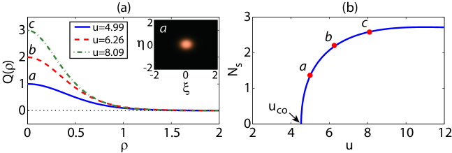
Figure 3: (Color online) (a): Profile $Q$ of the lowest-order ($l=0$) optical bullet for $u=4.99$ (solid line, labeled by “a”), 6.26 (dashed line, labeled by “b”), and 8.09 (dot-dashed line, labeled by “c”). Inset: Intensity distribution of the optical bullet for $u=4.99$ in the $(\xi,\eta)$ plane (corresponding to the profile “a”). (b): The norm of the optical bullet $N_{s}$ as a function of $u$. The cutoff value of $u$ is $u_{\rm co}\approx 4.529$. The solid circles indicated by “a”, “b”, and “c” are relevant to the profiles “a”, “b”, and “c” in the panel (a).

is the result of numerical simulation for the lowest-order ($l=0$) optical bullet and its stability. Fig. 3(a) gives profile $Q$ of the optical bullets for different values of $u$. In the simulation, $P=10$ and $\beta=2$ in Eq. (17) for $l=0$ have been chosen. The solid, dashed, and dotted-dashed lines in Fig. 3(a) are for $u=4.99$, 6.26, and 8.09, respectively. The inset shows the intensity distribution of the optical bullet for $u=4.99$ in the ($\xi,\eta$) plane. We see that the optical-bullet amplitude grows when $u$ increases.

The norm of the optical bullet, defined by $N_{s}=2\pi\int_{0}^{\infty}Q^{2}(\rho)\rho d\rho$, is found to be a monotonically growing function of $u$, i.e. $\partial N_{s}/\partial u>0$ (see Fig. 3(b) ), which implies the optical bullet is stable according to Vakhitov-Kolokolov criterion VK . However, the optical bullet exists only for $u\geq u_{\rm co}$. The cutoff value $u_{\rm co}$ grows when the strength $P$ of the Bessel optical lattice potential increases, and the optical bullet’s norm vanishes for $u\rightarrow u_{\rm co}$. For $P=10$, we obtain $u_{\rm co}\approx 4.529$. The solid circles indicated by “a”, “b”, and “c” in the panel (b) are relevant to the profiles “a”, “b”, and “c” in the panel (a).

We have also found high-order (i.e. $l\geq 1$) optical bullets in the system, which are stable nonlinear localized solutions in the presence of the high-order ($l\geq 1$) Bessel optical lattice. Such high-order optical bullets are trapped in the rings of off-center radial maxima of the Bessel optical lattice, where the refractive index contributed by the optical lattice are maximum. An example of a 1-order optical bullet in the 1-order Bessel optical lattice (the corresponding light intensity has been illustrated in the right part of Fig. 1(c) ) has been shown in Fig. 4(a).

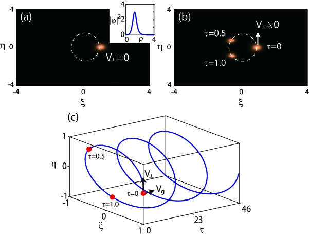
Figure 4: (Color online) (a): Intensity distribution in ($\xi,\eta$) plane of a stationary first-order ($l=1$) optical bullet without transverse velocity (i.e. $V_{\perp}=0$). The radius of the first ring (denoted by dashed circle) of the first-order Bessel lattice is $R_{L}\approx 0.92$. The inset shows the distribution $|\varphi|^{2}$ as a function of $\rho$. (b): Intensity distribution of a rotational first-order optical bullet with initial transverse velocity $V_{\perp}=1.07\times 10^{-7}$ $c$ for $\tau=0$, $0.5$, and $1.0$, respectively. (c): The helical motional trajectory (solid line) of the ultraslow optical bullet, which has the longitudinal velocity $V_{g}$ and the transverse velocity $V_{\perp}$. The solid circles indicate the position of the the optical bullet for $\tau=0$, $0.5$, and $1.0$, respectively.

The optical bullet locates in the first ring of the Bessel optical lattice, and has no transverse (i.e. $\xi$- and $\eta$-direction) velocity (i.e. $V_{\perp}=0$). The stability of the optical bullet has been verified using direct numerical simulations by considering the time evolution of the optical bullet with added random perturbations of relative amplitude up to 10% level.

The optical bullets obtained above have no transverse velocity, but, from expressions (13) and (14), they have a longitudinal velocity $V_{g}$ along the $z$-direction. We now show that, in fact, the high-order (i.e. $l\geq 1$) optical bullets can acquire a transverse velocity, and hence they can display a helical motion in the 3-dimensional space. This is possible because in each ring of the Bessel optical lattice the potential energy is degenerate, therefore an optical bullet will move around the ring with the minimum potential energy if an initial transverse velocity $V_{\perp}$ tangent to the ring is given rotary . Shown in Fig. 4(b) is the result of the rotation of a 1-order optical bullet with $V_{\perp}=1.07\times 10^{-7}$ $c$ for $\tau=0$, 0.5, and 1 (corresponding to $t$=0, 3, and 6 $\mu$s), respectively. Since now the optical bullet has the longitudinal velocity $V_{g}$ and also the transverse velocity $V_{\perp}$, it makes a helical motion in the 3-dimensional space. Fig. 4(c) shows such helical motion of the optical bullet, where the red solid circles indicate the position of the the optical bullet for $\tau=0$, $0.5$, and $1.0$, respectively. Because both $V_{g}$ and $V_{\perp}$ are much smaller than $c$, the nonlinear localized structure obtained here is indeed an ultraslow helical optical bullet.

V Acceleration of ultraslow helical optical bullets

Since the SG gradient magnetic fields can be used to change the propagating direction of optical beams KW , it can also be used to change the propagating velocity of optical pulses. We now study the acceleration of the ultraslow helical optical bullets. To this end, both the Bessel optical lattice and the time-dependent SG magnetic field must be applied simultaneously.

In order to describe the optical-bullet acceleration analytically, we assume that the ring-shaped trap formed by the Bessel optical lattice is narrow enough so that it ensures a quasi one-dimensional distribution of the light intensity of the optical bullet along the ring-shaped trap. On the other hand, the ring-shaped trap is also deep enough so that we can look for the solution with the form

$$\varphi(\tau,\rho,\theta)=\Phi(\rho)\Xi(\tau,\theta),$$ (18)

where $\Phi$ is the normalized ground state of the eigenvalue problem

$$\frac{1}{2\rho}\frac{d}{d\rho}\rho\frac{d}{d\rho}\Phi(\rho)+PJ_{l}^{2}(\sqrt{2\beta}\rho)\Phi(\rho)=E_{r}\Phi(\rho),$$ (19)

with $E_{r}$ the eigenvalue and $\Phi$ satisfying the normalization condition $\int_{0}^{\infty}\Phi^{2}\rho d\rho=1/(2\pi)$. Notice that the eigenvalue, and also $\Phi(\rho)$, depend on $l$. Here for simplicity we focus on the special situation $l=1$. After integrating over the variable $\rho$ and writing the equation into polar coordinates $(\rho,\,\theta)$, Eq. (15) becomes

$$i\frac{\partial}{\partial\tau}\Xi+\frac{R_{1}}{2}\frac{\partial^{2}}{\partial\theta^{2}}\Xi+[E_{r}+R_{2}F(\tau)\cos\theta]\Xi+\frac{R_{3}}{2\sqrt{\pi}\sigma}|\Xi|^{2}\Xi=0,$$ (20)

where $R_{j}$ ($j=1,2,3$) are given by $R_{1}=\int_{0}^{\infty}(\Phi^{2}/\rho)d\rho$, $R_{2}=\int_{0}^{\infty}\Phi^{2}\rho^{2}d\rho$, and $R_{3}=\int_{0}^{\infty}\Phi^{4}\rho^{2}d\rho$, respectively.

Let $\tilde{\Xi}=\sqrt{\frac{R_{3}}{2\sqrt{\pi}\sigma}}e^{-iE_{r}\tau}\Xi$, Eq. (20) can be further simplified to

$$i\frac{\partial}{\partial\tau}\tilde{\Xi}+\frac{1}{2}\frac{\partial^{2}}{\partial\vartheta^{2}}\tilde{\Xi}+\tilde{F}(\tau)\cos(\sqrt{R_{1}}\vartheta)\tilde{\Xi}+|\tilde{\Xi}|^{2}\tilde{\Xi}=0,$$ (21)

where $\vartheta=\theta/\sqrt{R_{1}}$ and $\tilde{F}=R_{2}F$. If the time-dependent gradient magnetic field is absent, i.e. $\tilde{F}(\tau)=0$, we can obtain the exact solution of Eq. (21) expressed by a Jacobi elliptic function, which, when taking the modulus of the Jacobi elliptic function as unity, reduces to a bright soliton moving with a constant velocity $v$:

$$\tilde{\Xi}(\tau,\vartheta)=e^{iv(\vartheta-v\tau)-i\Omega\tau}\eta\,{\rm sech}[\eta(\vartheta-v\tau)],$$ (22)

with $\Omega=-\eta^{2}/2+v^{2}/2$. We should bear in mind that $v$ in Eq. (22) is an angular velocity which is related to the transverse velocity by the relation $V_{\perp}=(v\sqrt{R_{1}})R_{L}$ with $R_{L}$ being the radius of the first (i.e. $l=1$) ring of the Bessel lattice. Returning to original variables, the soliton solution (22) reads

$$\Xi(\tau,\theta)=\sqrt{\frac{2\sqrt{\pi}\sigma}{R_{3}}}e^{iE_{r}\tau+iv(\theta/\sqrt{R_{1}}-v\tau)-i\omega\tau}\eta\,{\rm sech}\left[\eta\left(\frac{\theta}{\sqrt{R_{1}}}-v\tau\right)\right].$$ (23)

If the time-dependent SG gradient magnetic field is present, i.e. $\tilde{F}(\tau)\neq 0$, the velocity $v$ of the soliton is no longer preserved. Based on the solution (22), under adiabatic approximation the solution of the perturbed equation (20) can be assumed as the form

$$\tilde{\Xi}(\tau,\vartheta)=e^{iv(\tau)[\vartheta-\Theta(\tau)]-i\omega(\tau)\tau}\eta\,{\rm sech}(\eta[\vartheta-\Theta(\tau)]),$$ (24)

where $\Theta(\tau)$ is a time-dependent function yet to be determined. Using the variational method employed in ST , it is easy to obtain the equation of motion for $\Theta(\tau)$:

$$\frac{d^{2}\Theta}{d\tau^{2}}=-\sqrt{R_{1}}\tilde{F}(\tau)\sin(\sqrt{R_{1}}\Theta).$$ (25)

We are interested in the acceleration of the soliton when it undergoes a rotational motion along the ring. Actually, this acceleration can be achieved by using a steplike time dependence of $\tilde{F}(\tau)$ BK . To this end we assume that the soliton is initially centered at $\Theta(\tau=0)=0$ and require $\tilde{F}(\tau)$ to be zero for time intervals such that $\Theta(\tau)\in[2q\pi/\sqrt{R_{1}},(2q+1)\pi/\sqrt{R_{1}}]$ and to be a constant $\tilde{F}_{0}>0$ for $\Theta(\tau)\in[(2q+1)\pi/\sqrt{R_{1}},(2q+2)\pi/\sqrt{R_{1}}]$ with $q=0,1,2,\cdots$. In this way, the soliton acquires an acceleration at each time because the force contributed by the SG gradient magnetic field (see the right hand side of Eq. (25) ) is always positive.

Now our task is to find time intervals $T_{n}=[\tau_{n},\tau_{n+1}]$ ($n=0,\,1,\,2,\cdots$), with $\tau_{0}=0$, such that $\tilde{F}(\tau)=0$ for $\tau\in T_{2q}$ and $\tilde{F}(\tau)=\tilde{F}_{0}$ for $\tau\in T_{2q+1}$. During the time intervals $T_{2q}$, the soliton has to cross intervals $[2q\pi/\sqrt{R_{1}},(2q+1)\pi/\sqrt{R_{1}}]$ with a constant velocity while during the time intervals $T_{2q+1}$, the bullet has to cross intervals $[(2q+1)\pi/\sqrt{R_{1}},(2q+2)\pi/\sqrt{R_{1}}]$ with a growing velocity. By solving Eq. (25), we obtain

$$T_{2q}=\tau_{2q+1}-\tau_{2q}=\frac{\pi}{\sqrt{R_{1}}v_{2q}},$$ (26)

where $v_{2q}$ is the velocity at the point $2q\pi/\sqrt{R_{1}}$, and

$$T_{2q+1}=\tau_{2q+2}-\tau_{2q+1}=\int_{\pi/\sqrt{R_{1}}}^{2\pi/\sqrt{R_{1}}}\frac{d\Theta}{\sqrt{2\tilde{F}_{0}[\cos(\sqrt{R_{1}}\Theta)+1]+v_{2q+1}^{2}}},$$ (27)

where $v_{2q+1}$ is the velocity at the point $(2q+1)\pi/\sqrt{R_{1}}$. In addition, we have $v_{2q+1}=v_{2q}$ and $v_{2q+2}=\sqrt{4\tilde{F}_{0}+v_{2q+1}^{2}}$.

In a mechanical viewpoint, the acceleration of the soliton is caused by the magnetic force exerted by the SG gradient magnetic field, and hence the soliton possesses an effective magnetic moment KW ; HH . Note that the probe field is proportional to ${\cal A}$ (i.e. (13) ) which has a Gaussian factor $\psi$ (see (14) ), thus ${\cal A}$ is an optical bullet bounded in all three spatial directions and displays an accelerated motion along the first ring of the Bessel optical lattice. Since the optical bullet has also an untraslow motional velocity $V_{g}$ in the longitudinal (i.e. $z$) direction, its transverse acceleration can be observed for a very short medium length. Similarly, one can also realize a deceleration of the optical bullet along the ring by designing an appropriate force sequence, i.e. another steplike time dependence of $\tilde{F}(\tau)$.

In Fig. 5(a)

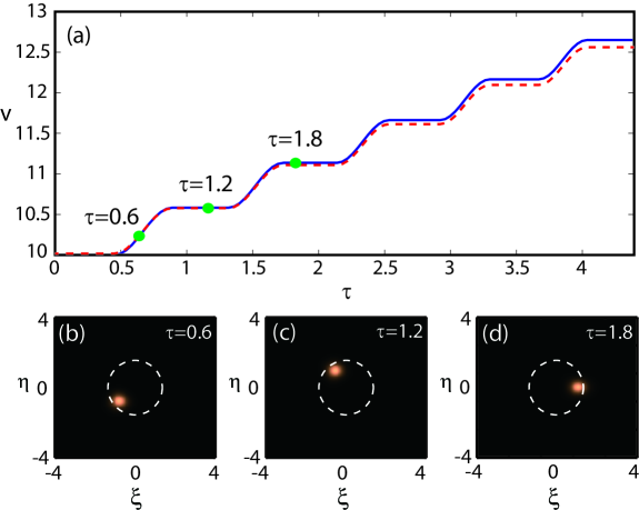
Figure 5: (Color online) Transverse acceleration of the optical bullet. (a): The angular velocity $v$ of the optical bullet rotating along the first ring of the first-order Bessel optical lattice as a function of $\tau$. The solid (dashed) line is the result obtained from Eq. (25) (Eq. (20) ) for $v_{0}=v(\tau=0)=10.0$ and $\tilde{F}_{0}=3.0$. The large solid circles correspond to $\tau=0.6$, 1.2, and 1.8 , respectively. (b), (c), (d): The light intensity distributions (positions) of the optical bullet in the first ring of the Bessel lattice (denoted by dashed circle with radius $R_{L}\approx 0.92$) for $\tau=0.6$, $1.2$, and $1.8$ in $(x,y)$ plane, respectively.

we compare the result of the solution obtained from Eq. (25) with the result of the numerical simulation from Eq. (20) for the first-order optical bullet with $v_{0}=10.0$ and $\tilde{F}_{0}=3.0$. During the simulation, $T_{2p}$ and $T_{2p+1}$ are obtained by Eqs. (26) and (27). One sees that the solution obtained from Eq. (25) (solid line) and the numerical simulation (dashed line) are matched quite well. The light intensity distributions (positions) of the optical bullet in the first ring of the Bessel lattice (denoted by dashed circle with radius $R_{L}\approx 0.92$) for $\tau=0.6$, 1.2, and 1.8 (corresponding to 3.6, 7.2, and 10.8 $\mu$s) are respectively depicted in the panels (b), (c), and (d) of Fig. 5, with the corresponding velocities indicated by the large solid circles in the panel (a). The transverse velocity of the optical bullet can accelerate from $v_{1}=10.0$ (i.e. $V_{\bot}\approx 1.8\times 10^{-7}$ $c$) to $v_{2}=10.6$ ($V_{\bot}\approx 1.9\times 10^{-7}$ $c$) in an atomic sample with the length $L=V_{g}T_{1}\tau_{0}\approx 0.85$ cm.

Using Poynting’s vector, it is easy to calculate the input power needed for generating the ultraslow helix optical bullets described above, which is estimated as $P\approx 0.2\times 10^{-3}$ mW. Thus for producing such optical bullets very low light intensity is required. This is drastic contrast to conventional optical media such as glass-based optical fibers, where ps or fs laser pulses are usually needed to reach a very high peak power to bring out the enough nonlinear effect needed for the formation of optical bullets Ait .

VI Conclusion

In this article, we have proposed a scheme to generate ultraslow (3+1)-dimensional helical optical bullets in a resonant three-level $\Lambda$-type atomic gas via EIT. We show that due to EIT effect the helical optical bullets can propagate with an ultraslow velocity up to $10^{-5}$ $c$ in the longitudinal direction and a slow rotational motion (with velocity $10^{-7}$ $c$) in transverse directions. The generation power of such optical bullets can be lowered to magnitude of microwatt, and their stability can be achieved by using a Bessel optical lattice formed by a far-detuned laser field. We have also demonstrated that the transverse rotational motion of the optical bullets can be accelerated by applying a time-dependent SG magnetic field. Because of the untraslow velocity in the longitudinal direction, a significant acceleration of the rotational motion of optical bullets may be observed for a very short medium length. Due to their interesting features, the ultraslow helical optical bullets obtained here may become candidates for light information processing and transmission at a very weak light level.

Appendix A The linear equations for each orders

The MB Eqs. (3) and (4) can be solved by standard method of multiple-scales huang . Substituting the expansion (7) into the Eqs. (3) and (4) and comparing the coefficients of $\epsilon^{m}$, we obtain the set of linear but inhomogeneous equations

$$i\left(\frac{\partial}{\partial z_{0}}+\frac{1}{c}\frac{\partial}{\partial t_{0}}\right)\Omega_{p}^{(m)}+\kappa_{13}\sigma_{31}^{(m)}=M^{(m)},$$ (28a)

$$\left(i\frac{\partial}{\partial t_{0}}+d_{21}^{(0)}\right)\sigma_{21}^{(m)}+\Omega_{c}^{\ast}\sigma_{31}^{(m)}=N^{(m)},$$ (28b)

$$\left(i\frac{\partial}{\partial t_{0}}+d_{31}^{(0)}\right)\sigma_{31}^{(m)}+\Omega_{p}^{(m)}+\Omega_{c}\sigma_{21}^{(m)}=P^{(m)},$$ (28c)

$$\left(i\frac{\partial}{\partial t_{0}}+d_{32}^{(0)}\right)\sigma_{32}^{(m)}+\Omega_{c}(\sigma_{11}^{(m)}+2\sigma_{22}^{(m)})=Q^{(m)},$$ (28d)

$$i\frac{\partial}{\partial t_{0}}\sigma_{11}^{(m)}+i\Gamma_{13}\sigma_{11}^{(m)}+i\Gamma_{13}\sigma_{22}^{(m)}=Y^{(m)},$$ (28e)

$$i\frac{\partial}{\partial t_{0}}\sigma_{22}^{(m)}+i\Gamma_{23}\sigma_{22}^{(m)}+i\Gamma_{23}\sigma_{11}^{(m)}+\Omega_{c}^{\ast}\sigma_{32}^{(m)}-\Omega_{c}\sigma_{32}^{\ast(m)}=Z^{(m)},$$ (28f)

where the explicit expressions of $M^{(m)}$, $N^{(m)}$, $P^{(m)}$, $Q^{(m)}$, $Y^{(m)}$ and $Z^{(m)}$ ($m=1,2,3,\cdots$) are given as

$$M^{(1)}=0,\,\,\,\,\,\,\,\,M^{(2)}=-i\left(\frac{\partial}{\partial z_{1}}+\frac{1}{c}\frac{\partial}{\partial t_{1}}\right)\Omega_{p}^{(1)},$$ (29a)

$$M^{(3)}=-i\left(\frac{\partial}{\partial z_{1}}+\frac{1}{c}\frac{\partial}{\partial t_{1}}\right)\Omega_{p}^{(2)}-i\frac{\partial}{\partial z_{2}}\Omega_{p}^{(1)}-\frac{c}{2\omega_{p}}\frac{\partial^{2}}{\partial x_{1}^{2}}\Omega_{p}^{(1)},$$ (29b)

$$N^{(1)}=0,\,\,\,\,\,\,\,\,N^{(2)}=-i\frac{\partial}{\partial t_{1}}\sigma_{21}^{(1)}+\Omega_{p}^{(1)}\sigma_{32}^{(1)\ast},$$ (29c)

$$N^{(3)}=-i\frac{\partial}{\partial t_{1}}\sigma_{21}^{(2)}+\Omega_{p}^{(1)}\sigma_{32}^{(2)\ast}+\Omega_{p}^{(2)}\sigma_{32}^{(1)\ast}-d_{21}^{(2)}\sigma_{21}^{(1)},$$ (29d)

$$P^{(1)}=0,\,\,\,\,\,\,\,\,P^{(2)}=-i\frac{\partial}{\partial t_{1}}\sigma_{31}^{(1)}-\Omega_{p}^{(1)}(2\sigma_{11}^{(1)}+\sigma_{22}^{(1)}),$$ (29e)

$$P^{(3)}=-i\frac{\partial}{\partial t_{1}}\sigma_{31}^{(2)}-\Omega_{p}^{(1)}(2\sigma_{11}^{(2)}+\sigma_{22}^{(2)})-\Omega_{p}^{(2)}(2\sigma_{11}^{(1)}+\sigma_{22}^{(1)})-d_{31}^{(2)}\sigma_{31}^{(1)},$$ (29f)

$$Q^{(1)}=0,\,\,\,\,\,\,\,\,Q^{(2)}=-i\frac{\partial}{\partial t_{1}}\sigma_{32}^{(1)}-\Omega_{p}^{(1)}\sigma_{21}^{(1)\ast},$$ (29g)

$$Q^{(3)}=-i\frac{\partial}{\partial t_{1}}\sigma_{32}^{(2)}-\Omega_{p}^{(1)}\sigma_{21}^{(2)\ast}-\Omega_{p}^{(2)}\sigma_{21}^{(1)\ast}--d_{32}^{(2)}\sigma_{32}^{(1)},$$ (29h)

$$Y^{(1)}=0,\,\,\,\,\,\,\,\,Y^{(2)}=-i\frac{\partial}{\partial t_{1}}\sigma_{11}^{(1)}-\Omega_{p}^{(1)\ast}\sigma_{31}^{(1)}+\Omega_{p}^{(1)}\sigma_{31}^{(1)\ast},$$ (29i)

$$Y^{(3)}=-i\frac{\partial}{\partial t_{1}}\sigma_{11}^{(2)}-\Omega_{p}^{(1)\ast}\sigma_{31}^{(2)}+\Omega_{p}^{(1)}\sigma_{31}^{(2)\ast}-\Omega_{p}^{(2)\ast}\sigma_{31}^{(1)}+\Omega_{p}^{(2)}\sigma_{31}^{(1)\ast},$$ (29j)

$$Z^{(1)}=0,\,\,\,\,\,\,\,\,Z^{(2)}=-i\frac{\partial}{\partial t_{1}}\sigma_{22}^{(1)},\,\,\,\,\,\,\,\,Z^{(3)}=-i\frac{\partial}{\partial t_{1}}\sigma_{22}^{(2)}.$$ (29k)

It is convenient to express Eq. (28) in the following form huang

$$\hat{L}\Omega_{p}^{(m)}=S^{(m)},$$ (30a)

$$\sigma_{31}^{(m)}=\frac{1}{\kappa_{13}}\left[M^{(m)}-i\left(\frac{\partial}{\partial z_{0}}+\frac{1}{c}\frac{\partial}{\partial t_{0}}\right)\Omega_{p}^{(m)}\right],$$ (30b)

$$\sigma_{21}^{(m)}=\left(i\frac{\partial}{\partial t_{0}}+d_{21}^{(0)}\right)^{-1}\left[N^{(m)}-\Omega_{c}^{\ast}\sigma_{31}^{(m)}\right],$$ (30c)

$$\sigma_{11}^{(m)}=\left[i\left(\frac{\partial}{\partial t_{0}}+\Gamma_{13}\right)\hat{L}_{2}-i\Gamma_{13}\hat{L}_{1}\right]^{-1}\left\{\hat{L}_{2}Y^{(m)}-i\Gamma_{13}\left[Z^{(m)}\right.\right.$$

$$\quad\quad\left.\left.-\Omega_{c}^{\ast}\left(i\frac{\partial}{\partial t_{0}}+d_{32}^{(0)}\right)^{-1}Q^{(m)}+\Omega_{c}\left(-i\frac{\partial}{\partial t_{0}}+d_{32}^{(0)\ast}\right)^{-1}Q^{(m)\ast}\right]\right\},$$ (30d)

$$\sigma_{22}^{(m)}=\frac{1}{\Gamma_{13}}\left[-iY^{(m)}-\left(\frac{\partial}{\partial t_{0}}+\Gamma_{13}\right)\sigma_{11}^{(m)}\right],$$ (30e)

$$\sigma_{32}^{(m)}=\left(i\frac{\partial}{\partial t_{0}}+d_{32}^{(0)}\right)^{-1}\left[Q^{(m)}-\Omega_{c}(\sigma_{11}^{(m)}+2\sigma_{22}^{(m)})\right],$$ (30f)

where operators $\hat{L}$, $\hat{L}_{1}$, $\hat{L}_{2}$ and $S^{(m)}$ are given as

$$\hat{L}=i\left(\frac{\partial}{\partial z_{0}}+\frac{1}{c}\frac{\partial}{\partial t_{0}}\right)+\kappa_{13}\left(i\frac{\partial}{\partial t_{0}}+d_{21}\right)\left[|\Omega_{c}|^{2}-\left(i\frac{\partial}{\partial t_{0}}+d_{21}\right)\left(i\frac{\partial}{\partial t_{0}}+d_{31}\right)\right]^{-1},$$

$$S^{(m)}=M^{(m)}-\kappa_{13}\left[|\Omega_{c}|^{2}-\left(i\frac{\partial}{\partial t_{0}}+d_{21}\right)\left(i\frac{\partial}{\partial t_{0}}+d_{31}\right)\right]^{-1}\left[\Omega_{c}N^{(m)}-\left(i\frac{\partial}{\partial t_{0}}+d_{21}\right)P^{(m)}\right],$$

$$\hat{L}_{1}=i\Gamma_{23}-|\Omega_{c}|^{2}\left[\left(i\frac{\partial}{\partial t_{0}}+d_{32}^{(0)}\right)^{-1}-\left(-i\frac{\partial}{\partial t_{0}}+d_{32}^{{(0)}\ast}\right)^{-1}\right],$$

$$\hat{L}_{2}=i\left(\frac{\partial}{\partial t_{0}}+\Gamma_{23}\right)-2|\Omega_{c}|^{2}\left[\left(i\frac{\partial}{\partial t_{0}}+d_{32}^{(0)}\right)^{-1}-\left(-i\frac{\partial}{\partial t_{0}}+d_{32}^{{(0)}\ast}\right)^{-1}\right].$$

Equation (30) can be solved order by order as shown in the main text.

References

- (1) M. Fleischhauer, A. Imamoglu, and J. P. Marangos, Rev. Mod. Phys. 77, 633 (2005), and references therein.
- (2) Y. Wu and L. Deng, Phys. Rev. Lett. 93, 143904 (2004).
- (3) G. Huang, L. Deng, and M. G. Payne, Phys. Rev. E 72, 016617 (2005).
- (4) C. Hang and G. Huang, Phys. Rev. A 77, 033830 (2008).
- (5) W.-X. Yang, A.-X. Chen, L.-G. Si, K. Jiang, X. Yang, and R.-K. Lee, Phys. Rev. A 81, 023814 (2010).
- (6) T. Hong, Phys. Rev. Lett. 90, 183901 (2003).
- (7) C. Hang, G. Huang, and L. Deng, Phys. Rev. E 74, 046601 (2006).
- (8) H. Michinel, M. J. Paz-Alonso, and V. M. Pérez-García, Phys. Rev. Lett. 96, 023903 (2006).
- (9) C. Hang, V. V. Konotop, and G. Huang, Phys. Rev. A 79, 033826 (2009).
- (10) H. Li, Y. Wu, and G. Huang, Phys. Rev. A 84, 033816 (2011).
- (11) R. Schlesser and A. Weis, Opt. Lett. 17, 1015 (1992).
- (12) R. Holzner, P. Eschle, S. Dangel, R. Richard, H. Schmid, U. Rusch, B. Röhricht, R. J. Ballagh, A. W. McCord, and W. J. Sandle, Phys. Rev. Lett. 78, 3451 (1997).
- (13) D. L. Zhou, L. Zhou, R. Q. Wang, S. Yi, and C. P. Sun, Phys. Rev. A 76, 055801 (2007).
- (14) L. Karpa and M. Weitz, Nat. Phys. 2, 332 (2006).
- (15) D. L. Zhou, L. Zhou, R. Q. Wang, S. Yi, and C. P. Sun, Phys. Rev. A 76, 055801 (2007).
- (16) Y. Li, C. Bruder, and C. P. Sun, Phys. Rev. Lett. 99, 130403 (2007).
- (17) Y. Guo, L. Zhou, L. Kuang, and C. P. Sun, Phys. Rev. A 78, 013833 (2008).
- (18) L. Karpa and M. Weitz, Phys. Rev. A 81, 041802 (2010).
- (19) C. Hang and G. Huang, Phys. Rev. A 86, 043809 (2012).
- (20) J. Javanainen, S. M. Paik, and S. M. Yoo, Phys. Rev. A 58, 580 (1998).
- (21) O. Dutta, M. Jääskeläinen, and P. Meystre, Phys. Rev. A 74, 023609 (2006).
- (22) C. Ryu, M. F. Andersen, P. Cladé, V. Natarajan, K. Helmerson, and W. D. Phillips, Phys. Rev. Lett. 99, 260401 (2007).
- (23) Y. V. Bludov and V. V. Konotop, Phys. Rev. A 75, 053614 (2007).
- (24) The frequency and wave number of the probe field are given by and respectively. Thus corresponds to the center frequency of the probe field.
- (25) Here ‘3’ denotes three spatial dimensions and ‘1’ denotes one temporal dimension.
- (26) M. G. Vakhitov and A. A. Kolokolov, Sov. J. Radiophys. Quantum Electron. 16, 783 (1973).
- (27) Y. V. Kartashov, V. A. Vysloukh, and L. Torner, Phys. Rev. Lett. 93, 093904 (2004).
- (28) H. Sakaguchi and M. Tamura, arXiv, nlin/0401027 (2004).
- (29) J. S. Aitchison, A. M. Weiner, Y. Silberberg, M. K. Oliver, J. L. Jackel, D. E. Leaird, E. M. Vogel, P. W. E. Smith, Opt. Lett. 15, 471 (1990).