Lateral density and arrival time distributions of Cherenkov photons in extensive air showers: a simulation study

Abstract

We have investigated some features of the density and arrival time distributions of Cherenkov photons in extensive air showers using the CORSIKA simulation package. The main thrust of this study is to see the effect of hadronic interaction models on the production pattern of Cherenkov photons with respect to distance from the shower core. Such studies are very important in ground based $\gamma$-ray astronomy for an effective rejection of huge cosmic ray background, where the atmospheric Cherenkov technique is being used extensively within the energy range of some hundred GeV to few TeV. We have found that for all primary particles, the density distribution patterns of Cherenkov photons follow the negative exponential function with different coefficients and slopes depending on the type of primary particle, its energy and the type of interaction model combinations. Whereas the arrival time distribution patterns of Cherenkov photons follow the function of the form $t(r)=t_{0}e^{\Gamma/r^{\lambda}}$, with different values of the function parameters. There is no significant effect of hadronic interaction model combinations on the density and arrival time distributions for the $\gamma$-ray primaries. However, for the hadronic showers, the effects of the model combinations are significant under different conditions.

I Introduction

The Atmospheric Cherenkov Technique (ACT) is being used extensively to detect the $\gamma$-rays emitted by celestial sources using the ground-based telescopes within the energy range of some hundred GeV to few TeV. This technique is based on the effective detection of Cherenkov photons emitted by the relativistic charged particles present in the Extensive Air Showers (EASs) initiated by the primary $\gamma$-rays in the atmosphere Hoffman ; Weekes ; Acharya . It is worthwhile to mention that, the celestial sources which emit $\gamma$-rays also emit Cosmic Rays (CRs). But CRs being charged particles, are deflected in the intergalactic magnetic fields and hence they reach us isotropically loosing the direction(s) of their source(s). However, as the $\gamma$-rays are neutral, by detecting them we can pinpoint the locations of such astrophysical sources.

As the ACT is an indirect method, detailed Monte Carlo simulation studies of atmospheric Cherenkov photons have to be carried out to estimate the energy of incident $\gamma$-ray. Also it is necessary to reject huge CR background as CRs also produce the EAS in the atmosphere like $\gamma$-rays but with a slight difference. The EAS originated from primary $\gamma$-rays are of pure electromagnetic in nature whereas those due to CRs are a mixture of electromagnetic and hadronic cascades. Many extensive studies have already been carried out on the arrival time as well as on the density distributions of atmospheric Cherenkov photons in EASs at the observation levels in the high as well as low energy regimes using available detailed simulation techniques Badran ; Versha . As the simulation study is interaction model dependent, it is also necessary to carry out the model dependent study for a reliable result. Although such type of studies have been also carried out extensively in the past, there are not many studies applicable particularly to high altitude observation levels. In keeping this point in mind, in this work we have studied the density and the arrival time distributions of Cherenkov photons in EASs of $\gamma$ and CR primaries, at different energies and at high altitude observation level, using different low and high energy hadronic interaction models available in the present version of the CORSIKA simulation package Heck .

CORSIKA is a detailed Monte Carlo simulation package to study the evolution and properties of extensive air showers in the atmosphere. This allows to simulate interactions and decays of nuclei, hadrons, muons, electrons and photons in the atmosphere up to energies of some 10²⁰eV. For the simulation of hadronic interactions, presently CORSIKA has seven options for high energy hadronic interaction models and three low energy hadronic interaction models. It uses EGS4 code Nelson for the simulation of electromagnetic component of the air shower Heck .

This paper is organized as follows. In the next section, we discuss in detail our simulation process. The section III is devoted for the details about the analysis of the simulated data and the results of the analysis. We summarize our work with conclusions and future outlook in the section IV.

II Simulation of atmospheric Cherenkov photons

We used CORSIKA 6.990 simulation package to simulate the Cherenkov photons emitted in the earth’s atmosphere by the relativistic charged particles of the EAS generated by $\gamma$ and CR primaries. We have considered two high energy hadronic interaction models, viz., QGSJET 01C and VENUS 4.12 together with all three low energy hadronic interaction models. These two sets of models are combined together in all six possible combinations, viz., QGSJET-GHEISHA, VENUS-GHEISHA, VENUS-UrQMD etc. to generate EASs for the vertically incident monoenergetic $\gamma$, proton and iron primaries. The motivation behind the choice of QGSJET01 and VENUS high energy hadronic interaction model is that, they are being used extensively in the simulation works of CR and $\gamma$-ray experiments Versha ; Oshima . Moreover, these two models are relatively old and both are based on Gribov-Regge theory Heck ; Goswami . However, it is important to have this type of study by using other high energy hadronic interaction models also.

Using all these six combinations of hadronic interaction models, few thousand showers of different energies are generated for $\gamma$-ray, proton and iron primaries. Details of the simulated sample are given in Table 1. The energies of these primaries selected here belong to the typical ACT energy range of respective primaries in terms of the equivalent number of Cherenkov photons produced by them. The altitude of HAGAR experiment at Hanle (longitude: 78^o 57^′ 51^′′ E, latitude: 32^o 46^′ 46^′′ N, altitude: 4270 m) Versha1 is used as the observational level in the generation of all these showers. However, to demonstrate the altitude effect in our study, we have also generated the showers using QGSJET-GHEISHA combination only over the Pachmarhi observation level (longitude: 78^o 26^′ E, latitude: 22^o 28^′ N, altitude: 1075 m), the site of PACT experiment Majumdar . Apart from all these showers, for specific purposes mentioned in the concerned sections, some more showers are generated for the Hanle observation level by using the VENUS-GHEISHA combination also.

Table 1: Number of generated showers for different primaries at different energies.

Primary particle	Energy	Number of Showers
$\gamma$-ray	100 GeV	10000
	500 GeV	5000
	1 TeV	2000
Proton	250 GeV	10000
	1 TeV	5000
	2 TeV	2000
Iron	5 TeV	5000
	10 TeV	2000

As we have used the QGSJET01 high energy hadronic interaction model in our study, it is important to compare the output of QGSJET01 with that of QGSJETII. For this purpose, we have also generated 2000 showers each for 1 TeV $\gamma$, 2 TeV proton and 10 TeV iron primary using the QGSJETII-GHEISHA model combination.

We have taken the detector geometry as a horizontal flat detector array, where there are 17 telescopes in the E – W direction with a separation of 25 m and 21 telescopes in the N – S direction with a separation of 20 m and the mirror area of each telescope as 9 m². So we have an array of 17$\times$21 i.e. 357 telescopes covering an area of 400 m$\times$400 m, which is equivalent to several 25 telescope sectors identical to PACT experiment Majumdar . Thus we have selected this detector geometry keeping in view of our earlier simulation works Versha . It doesn’t really matter as our idea is to study core distance dependence of parameters of vertical showers and this geometry is quite adequate to simulate vertical showers within the ACT energy range. However, it may be noted that, for inclined showers of ACT energy range, this geometry may not be sufficient as such showers cover more area depending on the angle of inclination for a given energy. The EASs produced by above mentioned primaries are considered to be incident vertically with their core at the centre of the array. For the longitudinal distribution of Cherenkov photons, photons are counted only in the step where they are emitted. Also the Cherenkov light emission angle is chosen as wavelength independent. The Cherenkov radiation produced within the specified bandwidth 200 – 650 nm by the charged secondaries is propagated to the ground. The position and time (with respect to the first interaction) of each photon hitting the detector on the observation level are recorded. The variable bunch size option of Cherenkov photon is set to ”5”, so that the size of the data file can be reduced. Multiple scattering length for e^- and e⁺ is decided by the parameter STEPFC in EGS code Nelson which has been set to 0.1. The low energy cutoff’s for the particle kinetic energy is chosen for hadrons, muons, electrons and photons as 3.0, 3.0, 0.003 and 0.003 GeV respectively. The US standard atmosphere parametrized by Linsley has been used US .

III Analysis and Results

For each shower, we have calculated the Cherenkov photon density at each detector. The arrival time of Cherenkov photons at each detector is calculated with respect to the first photon of the shower hitting the array. Since there are several photons hitting each detector, average of these arrival times is calculated for each detector. As there are shower to shower fluctuations in Cherenkov photon density and arrival time at each detector, the variation of Cherenkov photon density and arrival time with core distance is obtained by calculating average values over the specified number of showers. To demonstrate the fluctuations of photon density and arrival time as a function of core distance (or for each detector), the ratio of their r.m.s to mean values has been calculated. Moreover, to see the model dependent variations of these parameters clearly, we have calculated their percentage relative deviations with respect to the corresponding parameters for a reference model using the following formula:

$$\Delta_{\xi}=\frac{\xi_{mp}-\xi_{rp}}{\xi_{rp}}\times 100\%,$$ (1)

where $\Delta_{\xi}$ is the percentage relative deviation of the parameter, $\xi_{rp}$ is the reference model parameter and $\xi_{mp}$ is the given model parameter. Different features of Cherenkov photon density and arrival time distributions, and their model dependent behaviours are discussed in the following subsections:

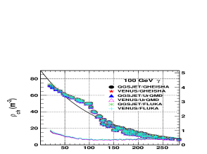
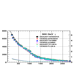
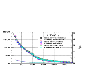
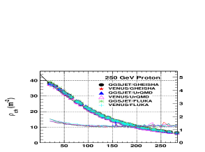
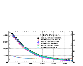
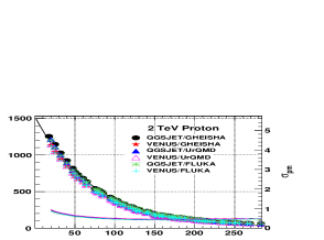
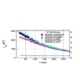
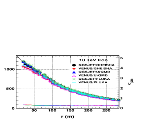
Figure 1: Variations in the average Cherenkov photon densities ($\rho_{ch}$) and their r.m.s. values per mean ($\sigma_{pm}$) with respect to distance from the shower core of different primaries for different high and low energy hadronic interaction models. The solid lines in respective plots indicate the results of the best fit function (2) for the QGSJET-GHEISHA combination. Fits are done by using the $\chi^{2}$-minimization method in the ROOT software Root platform.

III.1 Cherenkov photon density

III.1.1 General feature

Fig.1 shows the variations of average Cherenkov photon densities ($\rho_{ch}$s) and their r.m.s. values per mean ($\sigma_{pm}$) as a function of core distance for different combinations of low and high energy hadronic interaction models and for different shower primaries. It is seen that, the distribution of $\rho_{ch}$s falls off exponentially with core distance for all hadronic interaction model combinations, primary particles and their energies, as given by the equation

$$\rho_{ch}(r)=\rho_{0}\;e^{-\beta r},$$ (2)

where $\rho_{ch}(r)$ is the position dependent density function of Cherenkov photons, $r$ the distance from the shower core, $\rho_{0}$ the coefficient and $\beta$ the slope of the function. Values of $\rho_{0}$ and $\beta$ are different for different primaries. As an example, the best fit negative exponential functions for QGSJET-GHEISHA hadronic interaction model combination are indicated by solid lines in the plot. These fits are done by using the $\chi^{2}$-minimization method in the ROOT software Root platform. It needs to be mentioned that for 100 GeV $\gamma$-ray primary, the fit is not good due to the presence of hump at a core distance of about 100 m. Although the distributions follow the same mathematical function almost for all the cases with different coefficients and slopes, the geometry of the distributions is different for different primaries at a particular energy. It is seen that at a given energy, the distribution shows larger curvature for the $\gamma$-ray primary (except for 100 GeV) with higher values of coefficient and slope of the exponential function with a parameter $\beta$ smaller for iron primaries than for protons and increasing with energy.

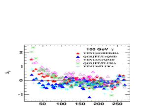
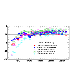
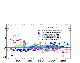
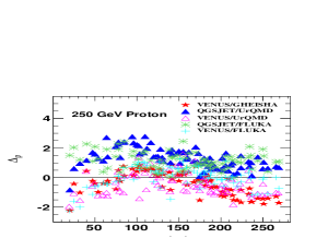
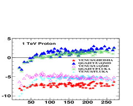
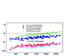
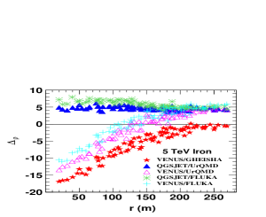
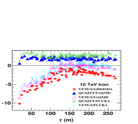
Figure 2: Variations of % relative Cherenkov photon densities ($\Delta_{\rho}$s) with respect to distance from the shower core of different primaries for different high and low energy hadronic interaction models. The horizontal solid lines in all plots indicate the QGSJET-GHEISHA model combination, which is considered as the reference for the calculation.

III.1.2 Dependence on hadronic interaction model

It is seen from the Fig.1 that, there is almost no visible effect of hadronic interaction models on the $\rho_{ch}$ distributions for the $\gamma$-ray primaries of energies upto 1 TeV. For proton primaries of energies upto 2 TeV, some slight discrepancies in densities are observed near the shower core upto the distance of $\leq$100 m, for different model combinations. In the case of iron primaries, the clear effect of hadronic interaction models is seen depending on the energy of the primary particle. In this case, QGSJET lead group of models (i.e. QGSJET-GHEISHA, QGSJET-UrQMD and QGSJET-FLUKA) have generated higher $\rho_{ch}$s than those generated by the VENUS lead group of models (i.e. VENUS-GHEISHA, VENUS-UrQMD and VENUS-FLUKA), in the region near shower core, depending on the energy of the primary particle. The magnitude of this difference and the effective core distance over which differences are seen is higher for the low energy primary particle.

To quantify the effect of different interaction models, we have calculated the % relative deviation of $\rho_{ch}$ ($\Delta_{\rho}$) for different model combinations taking QGSJET-GHEISHA as reference. Results are shown in the Fig.2. This choice of reference is arbitrary and it doest not effect the results as our aim is to see the effect of one model combination over the other. From this figure it is clear that, for the $\gamma$-ray primaries at all energies of our interest, there are no significant differences due to interaction models. Very near to the shower core ($<$50 m) some model combinations show deviations of $\sim$3% and beyond this distance the density deviations of all model combinations are within $\sim$$\pm$1%.

For the case of proton primary, the deviations from the reference combination are significant in comparison to $\gamma$-ray primary. The QGSJET lead group of models show deviations in densities within $\sim$$\pm$5%. At higher primary energies these deviations become increasingly negative. Within this group QGSJET-UrQMD combination gives maximum deviation in densities almost at all distances from the shower core for 1 TeV and 2 TeV primaries. Whereas for the VENUS lead group of models the density deviations are very large in comparison to deviations for QGSJET lead group of models. However, for the 250 GeV proton these deviations are insignificant as they are only within $\sim$$\pm$2%. On the other hand, for 1 TeV and 2 TeV proton primaries these deviations are negative: $\sim$-4% to -10% for 1 TeV and $\sim$-6% to -10% for 2 TeV. Within this group the maximum deviation is shown by different model combinations depending on the energy and the distance from the shower core.

Finally, in the case of iron primaries, the deviations are considerable for both types of model combinations. Unlike in the case proton primaries, the deviation is higher at lower primary energy. However, in this case the deviations for the QGSJET lead group of models are always positive and remain almost steady over all core distances. These deviations are $\sim$4 – 8% for the 5 TeV primary and $\sim$1 – 5% for the 10 TeV primary. On an average, here the maximum deviation is given by the QGSJET-FLUKA combination within QGSJET led group. The density deviations for VENUS lead group of models in this case vary from negative to positive values with core distance. For higher energies, deviations again become negative for higher core distances. This tendency is highest for VENUS-GHEISHA combination. For the 5 TeV primary deviations vary from $\sim$-17% to $\sim$6% with core distance whereas it is $\sim$-10% to $\sim$2% for the 10 TeV primary. On an average the VENUS-GHEISHA combination shows highest density deviations from the QGSJET-GHEISHA combination.

III.1.3 Behaviour of fluctuations

The values of $\sigma_{pm}$ of $\rho_{ch}$ for the $\gamma$-ray primaries decrease with increasing core distance upto a distance of $\sim$100 m and remain constant at larger core distances. This trend is seen for all energies and for all model combinations. This ratio decreases also with increasing energy (see Fig.1). There are no considerable differences due to different combinations of models. Although similar trend of variation of $\sigma_{pm}$ is seen in proton primaries, the values are higher compared to $\gamma$-ray primary for all model combinations. In case of iron primaries, $\sigma_{pm}$ is very small compared to proton primaries. For iron primaries also, values decrease with increasing energy. Moreover, it should be noted that, in this case the values of $\sigma_{pm}$ remain almost constant over all core distances. As for the case of $\gamma$-ray primaries, there are no considerable differences in $\sigma_{pm}$ due to different combinations of models for iron primaries.

III.1.4 Primary energy dependence

At a given energy, for all low and high energy hadronic interaction model combinations, the $\gamma$-ray primary produces maximum number of Cherenkov photons and the iron primary produces least number of it. To demonstrate this, we have plotted in the top and middle panels of the Fig.3, the $\rho_{ch}$ distributions with respect to the core distance produced by the $\gamma$, proton and iron primaries of 1 TeV and 2 TeV energies respectively. These are obtained by using the VENUS-GHEISHA model combination. Moreover, in the bottom panel of this figure, we have shown the variation of $\rho_{ch}$ at core distance of 100 m with respect to energy for the all primary particles. It is seen that, for the $\gamma$-ray primary, the $\rho_{ch}$ increases very rapidly and linearly with the primary energy. Whereas in the cases of proton and iron primaries, it increases slowly and non-linearly with the primary energy. The slowness and non-linearity effect is more prominent in the case of iron primary. These are due to the fact that, almost all the secondary EAS particles produced by $\gamma$-ray primary are electrons and positrons. Whereas the secondary particles produced by proton and iron primaries consist of not only electrons and positrons but muons and other hadronic particles as well. Moreover, in the case of iron nuclei primary, energy per nucleon is 56 times smaller than that for proton at a given energy. As electrons and positrons are the lightest particles, at a given energy more number of secondary particles of $\gamma$-ray primary cross threshold to produce Cherenkov photons compared to those produced by proton and iron primaries, with iron primary having the least number of such particles.

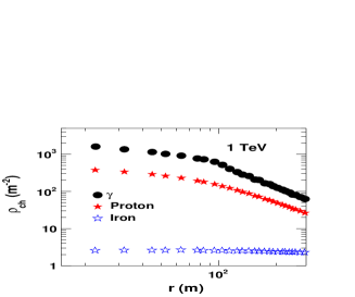
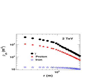
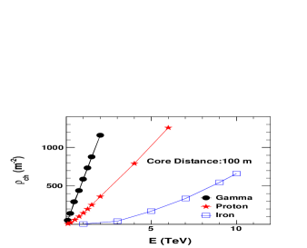
Figure 3: Top and middle panels: Distributions of $\rho_{ch}$s with respect to distance from the shower core of $\gamma$, proton and iron primaries at 1 TeV and 2 TeV energies given by the VENUS-GHEISHA model combination. Bottom panel: Variations of $\rho_{ch}$s with respect to primary energy at 100 m from the shower core of $\gamma$, proton and iron primaries for the same model combination as for the other two panels.

III.1.5 Altitude effect

To study the effect of height of the observation level on the lateral distribution of $\rho_{ch}$, we have selected $\gamma$-ray, proton and iron nuclei initiated showers from our CORSIKA database for two observational levels, one at the height of 4270 m from mean sea level (i.e. at the altitude of Hanle) and the other at the height of 1075 m (i.e. at the altitude of Pachmarhi) (see Sec.I). We considered different energies for primaries for QGSJET-GHEISHA model combination. The results of this analysis are shown in the Fig.4. This figure shows that, at higher observation level near the shower core, all primaries at all energies, produced considerably higher number of Cherenkov photons than that produced at the lower observation level. This difference decreases with increasing core distance and then at a particular core distance depending on the primary particle and its energy, the density become almost equal for both the observational levels. For the $\gamma$-ray primary, this distance is $\sim$130 m at all energies, which is different for proton and iron primaries.

It is seen that at higher observation level, for the 100 GeV $\gamma$-ray primary, the rate of decrease of the $\rho_{ch}$ with core distance is slower upto a core distance of $\sim$100 m and faster at larger core distances. Because of this behaviour a clear hump is seen for the 100 GeV $\gamma$-ray primary at a core distance of $\sim$100 m.

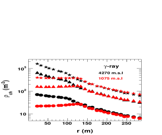
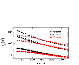
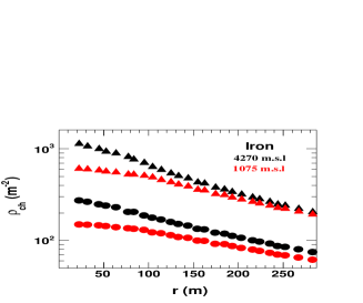
Figure 4: Distributions of $\rho_{ch}$s with respect to distance from the shower core of $\gamma$, proton and iron primaries at different energies given by the QGSJET-GHEISHA model combination over the observation levels of Hanle (black symbols) and Pachmarhi (red symbols). In the respective plots, $\bullet$/$\bullet$ indicates for 100 GeV $\gamma$, 250 GeV proton and 5 TeV iron primaries; $\blacktriangle$/$\blacktriangle$ indicates for 500 GeV $\gamma$, 1 TeV proton and 10 TeV iron primaries; and $\bigstar$/$\bigstar$ indicates for 1 TeV $\gamma$ and 2 TeV proton primaries.

     

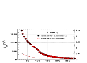
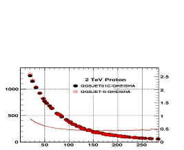
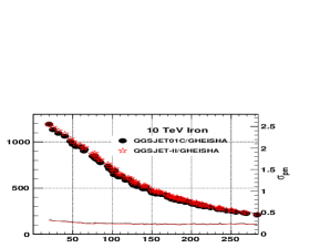
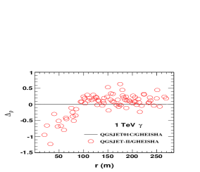
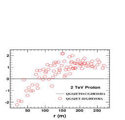
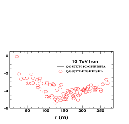
Figure 5: Top panels: Distributions of $\rho_{ch}$ with respect to distance from the shower core for 1 TeV $\gamma$, 2 TeV proton and 10 TeV iron primary particles obtained for the QGSJET01-GHEISHA and QGSJETII-GHEISHA model combinations. Bottom panels: $\Delta_{\rho}$ of densities with respect to distance from the shower core of primaries for QGSJETII-GHEISHA model combination from the densities of QGSJET01-GHEISHA combination.

At the lower observational level, the $\rho_{ch}$ remains constant with increasing core distance upto $\sim$130 m. At this core distance, hump is seen and $\rho_{ch}$ falls rapidly at larger core distances. In the case of proton and iron primaries, the $\rho_{ch}$ falls slowly with increasing core distance upto a distance of $\sim$100 m followed by faster decrease for larger core distances beyond this point, without forming any clearly visible hump. This behaviour of $\rho_{ch}$ at lower observational level for different primary particles is due to the fact that, most of the low energy soft component (electrons and positrons) of a shower gets absorbed as the shower travels a long distance (depending on the altitude of observational level) through the atmosphere to reach the lower observational level. The low energetic soft component of a shower is concentrated near to the shower core. As mentioned above, the $\gamma$-ray primary produces only the soft component shower, whereas the proton and iron primaries produce both the soft and hard components of the shower as well as other heavy particles depending on the energy of the concerned particles. Again, the iron primary has 56 times less energy per nucleon than proton primary of the same energy.

III.1.6 Comparison of QGSJET01 and QGSJETII

In this work, for convenience and as a convention we have used QGSJET01 as one of our high energy hadronic interaction models. Since the improved version of the QGSJET model is QGSJETII, it is important to compare results of the QGSJET01 and QGSJETII to verify the reliability of results from QGSJET01 model discussed so far. With this motivation, in the Fig.5 we have compared $\rho_{ch}$ distributions for 1 TeV $\gamma$, 2 TeV proton and 10 TeV iron primaries as obtained by using QGSJET01-GHEISHA and QGSJETII-GHEISHA model combinations. These three primaries are used as the representatives of their categories for this comparison. It is clear from the figure that the difference of the QGSJET01 and QGSJETII models is very small as far as the $\rho_{ch}$ is concerned. In fact, for the $\gamma$-ray primary there is no real difference between these two models as the $\rho_{ch}$ agrees within $\sim$1% at all core distances. For the proton primary the agreement is within $\sim$$\pm$2%. On the other hand for the iron primary the deviations range from 0 to $\sim$-5%, which are also negligible in comparison to deviation of other model combinations discussed above for this primary.

III.2 Arrival time of Cherenkov photons

III.2.1 General feature

The variation of mean arrival time of Cherenkov photons ($t_{ch}$) with respect to core distance is studied for all six combinations of low and high energy hadronic interaction models. These are shown in the Fig.6 for different primaries and their energies. It is observed that, the shower front is nearly spherical in shape for all primary particles, energies and model combinations. However, near shower core (core distance $\leq$50 m), the increase of the $t_{ch}$ with respect to core distance is comparatively slow, as a result the shape of the distribution deviates slightly from the spherical symmetry. This deviation increases with decreasing energy and increasing mass of the primary particle. Also, at a given energy, the deviation is more noticeable for the hadronic primaries. We have also found that, all these $t_{ch}$ distributions, irrespective of primary particles, their energies and the combinations of hadronic interaction models, follow the pattern as given by the function,

$$t_{ch}(r)=t_{0}e^{\Gamma/r^{\lambda}},$$ (3)

where $t_{ch}(r)$ is the position dependent arrival time, $r$ is the distance from the shower core, $t_{0}$, $\Gamma$ and $\lambda$ are constant parameters of the function. The values of these constant parameters depend on the type and energy of the primary particle for a given combination of low and high energy hadronic interaction models. In this figure, as an example, we have shown the best fit functions to the data from the QGSJET-GHEISHA combination as solid lines. Fits are done by using same method as mentioned in the density subsection.

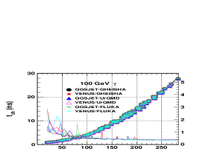
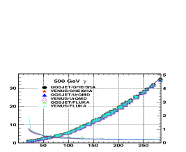
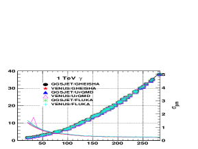
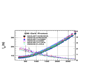
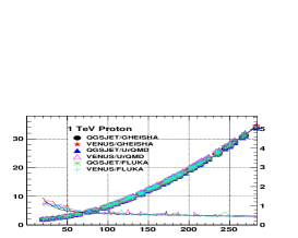
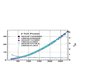
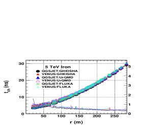
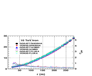
Figure 6: Variations of average arrival times of Cherenkov photons ($t_{ch}$) and their $\sigma_{pm}$ with respect to distance from the shower core of different primaries at different energies, given by different combinations of high and low energy hadronic interaction models. The solids line indicate the results of the best fitted function (3) to the respective plots for QGSJET-GHEISHA combination. Fits are done by using the $\chi^{2}$-minimization method in the ROOT software Root platform.

III.2.2 Dependence on hadronic interaction model

There are no visible differences in $t_{ch}$, produced by different combinations of low and high energy hadronic interaction models, in the case of $\gamma$-ray primary at all energies, as shown in the Fig.6. But, in the cases of 250 GeV proton and 5 TeV iron primaries, the noticeable differences due to model combinations are seen. For the 250 GeV proton primary the VENUS lead group of models give consistently higher $t_{ch}$ than the QGSJET lead group for all core distances. The difference is more prominent near shower core. Whereas in the case of 5 TeV iron primary, the difference is clearly noticeable for near core distance only, where the VENUS lead group of models give higher arrival time than the QGSJET lead group.

As in the case of $\rho_{ch}$, to see differences due to combination of models chosen, we study the relative deviations in the $t_{ch}$s considering QGSJET-GHEISHA combination as the reference. Fig.7 shows the % relative deviations of the arrival time ($\Delta_{t}$) of shower front for various model combinations for various monoenergetic primary particles as a function of the core distance. From the Fig.7 it is clear that, the differences due to different model combinations are small (0 to $\sim$$\pm$8%) for the $\gamma$-ray primaries. For all these primaries, the differences above 50 m core distances are negligible ($<$$\pm$ 2%) for all the models combinations except for one case, VENUS-GHEISHA combination with 1 TeV $\gamma$-rays. For this case, the deviation is the highest, which is upto -8% near the shower core and negligible only above 100 m core distances. Thus there is no particular trend of deviations of arrival times on the basis of model combination and all model combinations almost agree with the QGSJET-GHEISHA combination, at all energies of $\gamma$-ray primary.

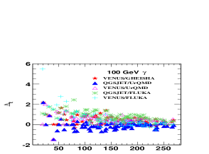
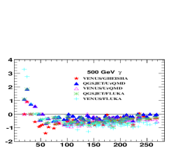
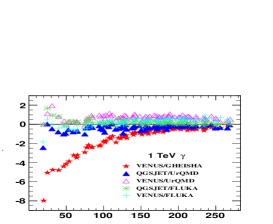
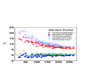
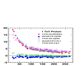
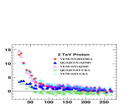
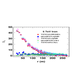
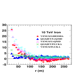
Figure 7: Variations of % relative arrival time deviations ($\Delta_{t}$s) of Cherenkov photons with respect to distance from the shower core of different primaries for different high and low energy hadronic interaction model combinations. The solid line in all plots indicates the values of the QGSJET-GHEISHA model combination. The QGSJET-GHEISHA model combination is considered as the reference for the calculation.

For proton and iron primaries the VENUS lead group of model combinations differ appreciably from the QGSJET-GHEISHA combination, depending on the energy and the type of primary particle. The prominence of these deviations increases with decreasing primary energy and with decreasing distance from shower core. For 250 GeV proton primary, the VENUS lead group of models produced $\sim$5 to 25% longer arrival times than those produced by QGSJET-GHEISHA combination, with a gradually decreasing trend with the increasing core distance. For 1 TeV and 2 TeV proton primaries this group of models produced $\sim$1 to 20% and $\sim$$\pm$ 1 to 15% longer arrival times respectively than the reference model combination. But in these two cases the time differences decrease very fast upto the core distance $\sim$100 m. Beyond this distance the arrival time differences become gradually negligible with increasing core distance. On an average, in this group of model combinations, the VENUS-FLUKA combination generates highest $\Delta_{t}$s over all core distances for the proton primaries. The trend due to the VENUS lead group of model combinations for the iron primaries is almost similar to that of proton primaries. However, here the $\Delta_{t}$s near the shower core are very large in comparison to proton primaries. For instance the $\Delta_{t}$s nearest to the shower cores of 5 TeV and 10 TeV iron primaries are $\sim$48% and $\sim$29% respectively. In the cases of iron primaries also, on an average the VENUS-FLUKA combination generates highest $\Delta_{t}$s over all core distances. For the QGSJET lead group of model combinations, the $\Delta_{t}$s are very small for all energies of proton and iron primary particles, as in the case of the $\gamma$-ray primary. This group of model combinations generate 0 to $\sim$$\pm$5% $\Delta_{t}$s for proton primaries and 0 to $\sim$$\pm$8% $\Delta_{t}$s for iron primaries than the reference model combination.

III.2.3 Behaviour of fluctuations

To observe the fluctuations in the $t_{ch}$ distributions, we have calculated the $\sigma_{pm}$ and plotted in the Fig.6 for different primaries, energies and model combinations. It is observed that, the fluctuation is large near the core for distances below 50 m. This is not clearly understandable. The fluctuation decreases with increasing core distance. The rate of decrease with the core distance is faster near the core and decreases at larger core distances for all primary particles, energies and model combinations except for 250 GeV proton primary, for which the rate of decrease of the fluctuations is almost same over all core distances. For a given primary particle, the fluctuation decreases with increasing energy of the particle. There is no particular model dependent trend seen. It should be noted that, for the proton primaries fluctuations produced by different model combinations are maximum amongst all primary particles. Moreover, as a whole, the differences in fluctuations, produced by different model combinations, are maximum near the shower core for all primary particles at all energies.

III.2.4 Primary energy dependence

For all the three types of primary particles, we have studied the variation of $t_{ch}$ with core distance for a constant energy. We have also studied the variation of $t_{ch}$ at core distance of 100 m as a function of primary energy. Results are shown in the Fig.8 for the VENUS-GHEISHA combination only.

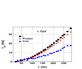
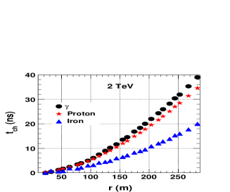
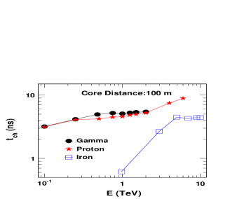
Figure 8: Top and middle panels: Distributions of offset normalised $t_{ch}$ with respect to distance from the shower core of $\gamma$, proton and iron primaries at 1 TeV and 2 TeV energies, as given by the VENUS-GHEISHA model combination. Bottom panel: Variations of offset normalised $t_{ch}$ with respect to primary energy at a distance 100 m from the shower core of $\gamma$, proton and iron primaries for the same model combination as for the other two panels.

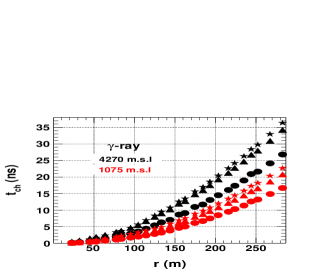
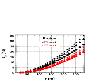
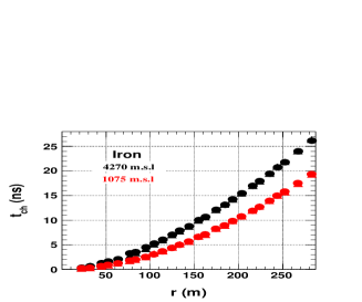
Figure 9: Distributions of offset normalised $t_{ch}$ with respect to distance from the shower core of $\gamma$, proton and iron primaries at different energies given by the QGSJET-GHEISHA model combination over the observation levels of Hanle (black symbols) and Pachmarhi (red symbols). In the respective plots, $\bullet$/$\bullet$ indicates for 100 GeV $\gamma$, 250 GeV proton and 5 TeV iron primaries; $\blacktriangle$/$\blacktriangle$ indicates for 500 GeV $\gamma$, 1 TeV proton and 10 TeV iron primaries; and $\bigstar$/$\bigstar$ indicates for 1 TeV $\gamma$ and 2 TeV proton primaries.

     

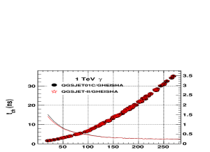
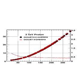
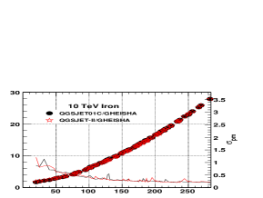
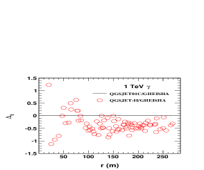
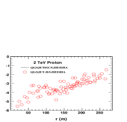
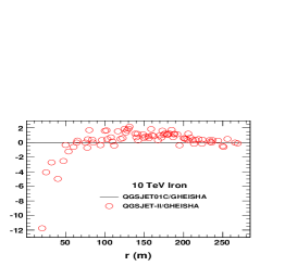
Figure 10: Top panels: Distributions of $t_{ch}$ with respect to distance from the shower core for 1 TeV $\gamma$, 2 TeV proton and 10 TeV iron primary particles obtained for the QGSJET01-GHEISHA and QGSJETII-GHEISHA model combinations. Bottom panels: $\Delta_{t}$ of $t_{ch}$ with respect to distance from the shower core of these primaries for QGSJETII-GHEISHA model combination from the $t_{ch}$ of QGSJET01-GHEISHA combination.

We see that, at a given energy, on an average, Cherenkov photons from a shower initiated by a $\gamma$-ray take the longest time to reach the observation level. This time is shortest for the iron primary. The difference in the $t_{ch}$ for showers initiated by $\gamma$-ray and proton, at a given core distance is very small. While the difference is quite large for the iron primary. At a given core distance, the $t_{ch}$ increases with increasing energy of the primary particle upto certain energy, depending upon the type of primary particle. For the $\gamma$-ray primary this energy is $\sim$2 TeV and for the iron primary it is $\sim$5 TeV. But for the proton primary it will be greater than 6 TeV (see the bottom panel of the Fig.8).

As discussed in the density subsection, at a given primary energy, the $\gamma$-ray primary produces highest number and iron primary produces least number of Cherenkov photons. While number of Cherenkov photons produced by proton primary is slightly less than that produced by the $\gamma$-ray primary. So the angular and hence arrival time distributions of Cherenkov photons with respect to the first arriving particle over the observation level is much wider for the $\gamma$-ray primary than that for iron and slightly wider that that for proton primary. This arrival time distribution also producing the observed effect on the time distribution.

III.2.5 Altitude effect

The effect of altitude of the observational level on the $t_{ch}$ distribution is also studied and is shown in the Fig.9. It is clear from this figure that, for all primary particles at all energies, the average arrival time of Cherenkov photons’ shower is shorter over the lower observation level than that over the higher observation level with respect to the same first arriving photon. Over the same observation level it is longer for higher energy primary than that for the low energy primary as already mentioned above. The difference between this arrival time of two primaries decreases with increasing energy and mass of the primary particle.

When a shower has to a travel long distance to arrive at lower observation level, most of the low energetic particles get absorbed in the atmosphere, leaving only high energetic particles having their energies almost in same order of magnitude. Consequently, the relative time differences of different particles, arrive on the observation level with the first arriving particle are comparatively smaller than that are observed on the observation level at higher altitude. So the $t_{ch}$ at lower observation level are smaller in magnitudes than the $t_{ch}$ at higher observational level.

III.2.6 Comparison of QGSJET01 and QGSJETII

We have also studied the difference in $t_{ch}$ produced by QGSJET01-GHEISHA and QGSJETII-GHEISHA model combinations. The results of this study is shown in the Fig.10. It is seen from the figure that, for the $\gamma$-ray primary there is no any real difference between these two models as the deviations of the $t_{ch}$s generated by these two models are only 0 to $\sim$$\pm$1.1% over all core distances. For the proton primary the deviations are $\sim$-2.5 to $\sim$5.5%, which are negligible. On the other hand for the iron primary the effective deviations range from 0 to $\sim$$\pm$5%, which are also negligible in comparison deviation of other model combinations discussed above for this primary.

IV Summary and conclusion

In view of the importance in the ACT and lack of sufficient works applicable to high altitude observation sites, we have made an elaborate study on the density and arrival time distributions of Cherenkov photons in EAS using the CORSIKA 6.990 simulation package Heck . Summary of this study and consequent conclusions can be made as follows:

The lateral density and arrival time distributions of Cherenkov photons follow a negative exponential function and a function of the form $t(r)=t_{0}e^{\Gamma/r^{\lambda}}$ respectively for all primary particles, energies and model combinations. As these functions’ parameters are different, the geometries of these distributions are obviously different depending upon the energy and mass of the primary particle. These parametrisations show that the analytical descriptions of the lateral density and arrival time distributions of Cherenkov photons are possible within some uncertainty. The full scale of such parametrization as a function of energy and shower angle would be useful for analysis of data of $\gamma$-ray telescopes because, it will help to disentangle the $\gamma$-ray showers from the hadronic showers over a given observation level.

These distributions of density and arrival time of Cherenkov photons as a function of core distance for the $\gamma$-ray showers are almost independent of hadronic interaction models, whereas that for the proton and iron showers depend on the hadronic interaction models on the basis of the type of models (low and high energy), the energy of primary particle and the distance from the shower core. In most of the cases the model dependence is significant for the iron showers. The systematic effect of the hadronic interaction model dependence has to be taken into account when assessing the effectiveness of background rejection for a $\gamma$-ray telescope. Moreover, from the study of shower to shower fluctuations ($\Delta_{pm}$) of Cherenkov photons’ density and arrival time it is clear that they are almost independent of hadronic interaction models, but depend on the energy and type of the primary particle, number of shower samples used for the analysis and the location of detectors. These are very important inference to be taken into care on the estimation of systematic uncertainties in a real $\gamma$-ray astronomy observation.

The energy dependent variation of Cherenkov photons’ density shows that to get the equivalent numbers of Cherenkov photons from different primary particles, the energy of the particles must be increased to several times with increasing mass of them. This explains why we have chosen different specific energies for different primaries as mentioned in the Sec.II. Similarly, from the study of the altitude effect, i.e. the comparison of lateral distributions of Cherenkov photons at two observation levels, we can conclude that as we go to the higher observation levels, it is possible to detect low energy $\gamma$-ray signals from a source as well as possible to do the $\gamma$-ray astronomy with a much smaller telescope system than at lower observation level.

As mentioned above the full scale parametrisation of the density and arrival time distributions of Cherenkov photons for different primary is important for the analysis of $\gamma$-ray observation data, so in future we are planning to perform such full parametrization for the HAGAR telescope site for the effective analysis of the HAGAR telescope Versha1 data. Again, since in this work we have considered the energy only upto 10 TeV, hence we will extend our future work upto 100 TeV, the more relevant energy range of $\gamma$-ray astronomy. Furthermore, as the pattern of angular distribution of Cherenkov photons for different primaries is another crucial parameter for separation of hadron showers from the $\gamma$-ray showers, we will take up this issue also for our future study.

References

- (1) René A. Ong, Phys. Reports 305, 93 (1998), C. M. Hoffman and C. Sinnis, Rev. Mod. Phys. 71, 897 (1999).
- (2) T. C. Weekes, astroph/0811.1197v1 (2009).
- (3) P. N. Bhat, Bull. Astr. Soc. India 30, 135 (2002); B. S. Acharya, 29th ICRC, 10, 271 (2005).
- (4) H. M. Badran, T. C. Weekes, Astropart. Phys. 7, 307 (1997); Hervé Cabot et al., Astropart. Phys. 9, 269 (1998);
- (5) V. R. Chitnis,P. N. Bhat, Astropart. Phys. 9, 45 (1998); V. R. Chitnis, P. N. Bhat, Astropart. Phys. 12, 45 (1999); V. R. Chitnis, P. N. Bhat, Astropart. Phys. 15, 29 (2001); M. A. Rahman et al., Exper. Astron. 11, 113 (2001); V. R. Chitnis, P. N. Bhat, BASI 30, 351 (2002); V. R. Chitnis, P. N. Bhat, Exper. Astron. 13, 77 (2002);
- (6) J. Knapp, D. Heck, EAS Simulation with CORSIKA V 6990: A User’s Guide (1998); D. Heck et al., Report FZKA 6019 (1998), Forschungszentrum Karlsruhe; http://wwwik.fzk.de/corsika/physicsdescription/corsika phys.html
- (7) W. R. Nelson, H. Hirayamal, D. W. O. Rogers, The EGS4 Code System, SLAC Report 265 (1985).
- (8) A. Oshima, S.R. Dugad, U.D. Goswami, S.K. Gupta et al., Astropart. Phys. 33, 97 (2010).
- (9) U.D. Goswami, Astropart. Phys. 28, 251 (2007).
- (10) V. R. Chitnis et al., Proc. 31st ICRC, Lodz, icrc0696 (2009); R. J. Britto et al., Astrophys. Space Sci. Trans. 7, 501 (2011).
- (11) P. Majumdar et al., Astropart. Phys. 18, 333 (2003); V. R. Chitnis et al. 27th ICRC, Hamburg (Germany), 2001.
- (12) US Standard Atmosphere (US Govt. Printing Office, Washington, 1962)
- (13) http://root.cern.ch