A new cosmological distance measure using AGN X-ray variability

Abstract

We report the discovery of a luminosity distance estimator using Active Galactic Nuclei (AGN). We combine the correlation between the X-ray variability amplitude and the Black Hole (BH) mass with the single epoch spectra BH mass estimates which depend on the AGN luminosity and the line width emitted by the broad line region. We demonstrate that significant correlations do exist which allows one to predict the AGN (optical or X-ray) luminosity as a function of the AGN X-ray variability and either the H$\beta$ or the Pa$\beta$ line widths. In the best case, when the Pa$\beta$ is used, the relationship has an intrinsic dispersion of $\sim$0.6 dex. Although intrinsically more disperse than Supernovae Ia, this relation constitutes an alternative distance indicator potentially able to probe, in an independent way, the expansion history of the Universe. With this respect, we show that the new mission concept Athena should be able to measure the X-ray variability of hundreds of AGN and then constrain the distance modulus with uncertainties of 0.1 mag up to $z\sim 0.6$. We also discuss how, using a new dedicated wide field X-ray telescope able to measure the variability of thousands of AGNs, our estimator has the prospect to become a cosmological probe even more sensitive than current Supernovae Ia samples.

1. Introduction

One of the most important results on observational cosmology is the discovery, using type Ia supernovae (SNeIa) as standard candles, of the accelerating expansion of the Universe (Riess et al., 1998; Perlmutter et al., 1999). However, the use of SNeIa is difficult beyond $z\sim 1$ and limited up to $z\sim 2$ (e.g. Rubin et al., 2013). It is therefore of paramount importance to calibrate other independent distance indicators able to measure the Universe expansion. It would be even better if such a method would be able to probe even beyond these redshifts, where the differences among various cosmological models are larger.

Given their high luminosities, since their discovery there have been several studies on the use of Active Galactic Nuclei (AGN) as standard candles or rulers (Baldwin, 1977; Rudge & Raine, 1999; Collier et al., 1999; Elvis & Karovska, 2002). More recently, also thanks to a better understanding of the AGN structure, more promising methods have been presented (see Marziani & Sulentic (2013) and the review therein). For example, many authors (e.g. Watson et al., 2011) use the tight relationship between the luminosity of an AGN and the radius of its Broad Line Region (BLR) established via reverberation mapping to determine the luminosity distances. On the other hand, Wang et al. (2013) suggest that super-Eddington accreting massive BH may reach saturated luminosities, which then provide a new tool for estimating cosmological distances. Besides AGN, gamma ray bursts (GRB) have been used as standard candles, however their low identification rate makes their use difficult (e.g. Schaefer, 2007, and references therein).

Here we propose a new method to predict the AGN luminosity based on the combination of the virial relations, which allow to derive the BH mass (M_BH) from the AGN luminosity and the width of the lines emitted from the BLR, and the well established anti-correlation between M_BH and the X-ray variability amplitude.

2. Method

Table 1Calibration Sample

Name	z	$\sigma^{2}_{\rm rms}$	low-err${}_{\sigma^{2}_{\rm rms}}$	up-err${}_{\sigma^{2}_{\rm rms}}$	logL5100	logLx	FWHMHβ	FWHMPaβ	Ref
					erg s-1	erg s-1	km s-1	km s-1
(1)	(2)	(3)	(4)	(5)	(6)	(7)	(8)	(9)	(10)
1E0919+515	0.1610	0.078000	0.052439	0.091463	44.29	43.43	1980	…	a
1H0707-495	0.0411	0.219000	0.027439	0.030488	…	42.67	1000	…	b
3C120	0.0330	0.000210	0.000116	0.000183	44.09	44.06	2327	2733	c
3C273	0.1583	0.000027	0.000022	0.000024	46.02	45.80	3500	2916	d
ARK120	0.0323	0.000290	0.000249	0.000427	44.37	43.96	6120	5114	d
ARK564	0.0247	0.044000	0.008537	0.012195	…	43.37	…	1616
ESO198-G24	0.0455	0.000780	0.000445	0.000671	…	43.70	6400	…	e
HE1029-1401	0.0860	0.001000	0.000610	0.001159	45.27	44.54	7500	…	f
HE1143-1810	0.0330	0.000690	0.000463	0.000671	…	43.85	2400	…	e
IC4329A	0.0161	0.000168	0.000084	0.000137	42.89	43.75	5964	…	c
IRAS13349+2438	0.1076	0.007300	0.002256	0.004268	44.64	43.87	2800	…	g
IRAS17020+4544	0.0610	0.016400	0.004695	0.007317	…	43.71	1040	…	h
IRASF12397+3333	0.0450	0.009500	0.003049	0.004878	43.36	43.38	1640	…	g
MCG-6-30-15	0.0077	0.035200	0.005000	0.004878	42.86	42.75	2020	…	i
MRK110	0.0353	0.000398	0.000269	0.000410	43.63	43.91	2079	1918	d
MRK1502	0.0611	0.021300	0.005732	0.012195	44.79	43.65	1171	…	d
MRK279	0.0305	0.000275	0.000173	0.000238	43.82	43.78	5411	3568	d
MRK335	0.0258	0.015160	0.002382	0.002382	43.71	43.44	1841	1858	d
MRK509	0.0344	0.000296	0.000093	0.000091	43.91	44.02	3424	3077	l
MRK590	0.0264	0.002154	0.001468	0.002390	44.01	43.04	2627	3964	d
MRK766	0.0129	0.027787	0.003285	0.003285	43.31	42.94	1100	…	g
MRK841	0.0364	0.001700	0.001037	0.001829	43.64	43.49	6000	…	g
NGC3227	0.0039	0.008757	0.001976	0.004366	42.86	41.57	4445	2955	g
NGC3516	0.0088	0.003594	0.001015	0.001015	43.17	42.46	5236	4469	g
NGC3783	0.0097	0.005052	0.001217	0.001217	43.20	43.08	3555	…	d
NGC4051	0.0023	0.113421	0.012172	0.012172	41.47	41.44	1170	1681	l
NGC4151	0.0033	0.000890	0.000427	0.000915	42.58	42.53	6421	4667	d
NGC4395	0.0011	0.144050	0.031327	0.065367	…	40.21	1500	…	m
NGC4593	0.0090	0.009819	0.003163	0.006379	42.85	42.87	5143	3791	c
NGC5548	0.0172	0.000283	0.000173	0.000278	43.21	43.42	6300	6525	l
NGC7469	0.0163	0.002942	0.000641	0.001363	43.74	43.23	2639	1792	d
PDS456	0.1840	0.004800	0.001402	0.001220	…	44.90	3974	2068	n
PG0844+349	0.0640	0.019000	0.010366	0.024390	…	43.70	…	2410
PG1211+143	0.0809	0.010500	0.002683	0.005488	44.42	43.73	1900	…	g
PG1440+356	0.0791	0.006400	0.002927	0.004878	44.46	43.61	1630	…	g
RE1034+396	0.0421	0.018000	0.006707	0.009756	43.18	42.53	700	…	g
RXJ0057.2-2223	0.0620	0.023000	0.010366	0.018293	44.27	43.65	970	…	g
RXJ0136.9-3510	0.2890	0.064000	0.026220	0.054878	…	44.34	1320	…	o
RXJ0323.2-4931	0.0710	0.009000	0.006707	0.010976	43.58	43.21	1680	…	g
SDSSJ135724.51+652505.9	0.1063	0.073000	0.044512	0.054878	43.14	42.90	737	…	p

Note. — Columns 3, 4 and 5: Excess variance, $\sigma^{2}_{\rm rms}$, and lower and upper errors at 1$\sigma$ confidence level from Ponti et al. (2012). Column 6: $\lambda L_{\lambda}$ continuum luminosity at 5100Å. Column 7: 2-10 keV intrinsic luminosity. Column 9: from Landt et al. (2008, 2013). Column 10: References for FWHM_Hβ and L₅₁₀₀: a) Jin et al. (2012), b) Boller et al. (1996), c) Assef et al. (2012), d) Vestergaard & Peterson (2006), e) Winkler (1992), f) McLure & Dunlop (2001), g) Grupe et al. (2004), h) Leighly (1999), i) McHardy et al. (2005), l) Wandel et al. (1999), m) Kraemer et al. (1999), n) Torres et al. (1997), o) Grupe et al. (1999), p) Zhou et al. (2006).

The method which uses single epoch (SE) spectra (in the optical or near infrared bands) to measure M_BH (e.g. Wandel et al., 1999; McLure & Jarvis, 2002; Vestergaard & Osmer, 2009; Landt et al., 2013) is now well established. By combining the velocity, $\Delta V$, of the BLR clouds (assuming Keplerian orbits) along with their distance R it is possible to determine the total mass contained within the BLR (which is dominated by the BH) using

$${\rm M}_{\rm BH}={{f\Delta{\rm V}^{2}{\rm R}}\over{\rm G}},$$ (1)

where G is the gravitational constant, $\Delta{\rm V}^{2}{\rm R}$ is the virial product and f is a factor which depends on the geometric and kinematic structure of the BLR. These techniques derive M_BH using SE spectra to measure $\Delta$V from the Full Width at Half Maximum (FWHM) of some of the BLR lines (typically: H_β or MgII2798Å or CIV1459Å) and R from either the continuum or the line luminosities, L, which have been proved to be proportional to R² (see Bentz et al., 2013, and references therein). Therefore, the SE estimates are based on relations of the type

$${\rm logM}_{\rm BH}=\alpha{\rm logL}+\beta{\rm log}\Delta V+\gamma,$$ (2)

where the values of the parameters $\alpha\sim 0.5$, $\beta\sim 2$ and $\gamma$ depend on the emission line of the BLR used. These relationships have typical uncertainties of $\sim$0.5 dex.

On the other hand, several studies have found a significant anti-correlation between M_BH and the X-rays variability (Nandra et al., 1997; Turner et al., 1999; O’Neill et al., 2005; McHardy et al., 2006; Gierliński et al., 2008; Zhou et al., 2010; Ponti et al., 2012; Kelly et al., 2013). Following Ponti et al. (2012) it results

$${\rm logM}_{\rm BH}=-k\cdot{\rm log}\sigma_{\rm rms}^{2}+w,$$ (3)

where $k\sim 0.8$ and $w$ are two constants which depend on the time scale and the energy range where the variable flux is measured. $\sigma^{2}_{rms}$ is the normalised excess variance variability estimator:

$$\sigma^{2}_{\rm rms}={1\over{N\mu^{2}}}\Sigma_{i=1}^{N}\left[(X_{i}-\mu)^{2}-\sigma_{i}^{2}\right],$$ (4)

where N is the number of time intervals where the fluxes (or the counts) $X_{i}$ are measured, $\mu$ is the mean of the N fluxes $X_{i}$ and $\sigma_{i}$ is the uncertainty on the i-th flux measure. According to X-ray variability studies on samples of AGN whose M_BH has been measured with reverberation mapping techniques, these kinds of relationships could have spreads as narrow as 0.2-0.4 dex (Zhou et al., 2010; Ponti et al., 2012; Kelly et al., 2013).

The origin of M_BH -$\sigma^{2}_{\rm rms}$relation (eq. 3) is to be found in the dependence on M_BH of the time-scales of what appears to be a universal shape of the AGN variability power spectral density (PSD). Indeed, the AGN X-ray PSDs are generally well modelled by two power laws, ${\rm P}(\nu)\propto 1/\nu^{n}$, where the PSD slope is $n\sim 1$ down to a break frequency $\nu_{b}$, that scales primarily with M_BH, and then steepens to $n\sim 2$ at larger frequencies. However, measuring the shape of the AGN X-ray PSD is very data demanding, requiring high quality data on many different time-scales. Therefore these studies are confined to a relatively small number of sources. On the contrary, the excess variance $\sigma^{2}_{\rm rms}$ is a robust estimator as it corresponds to the integral of the PSD on the time scales probed by the data. The scaling of the characteristic frequencies of the PSD with M_BH (and the roughly similar PSD normalisation at $\nu_{b}$) induces a dependence of the excess variance with M_BH (if computed at frequencies above $\nu_{b}$).

The two equations (2 and 3) used to estimate M_BH can be combined to derive the intrinsic AGN luminosity as a function of its X-ray variability, $\sigma_{rms}^{2}$, and line width, $\Delta V$:

$${\rm logL}=-{k\over\alpha}\cdot{\rm log}\sigma^{2}-{\beta\over\alpha}{\rm log}\Delta V+{\rm const},$$ (5)

which, if we (for the sake of simplicity) assume $\alpha=0.5$ and $\beta=2$, becomes

$${\rm logL}=-2k\cdot{\rm log}\sigma^{2}-4{\rm log}\Delta V+{\rm const}.$$ (6)

In this work we aim to verify if the above proposed relationship does work and then calibrate it. It should be noted that, in many previous studies, a correlation between the AGN luminosity and X-ray variability has been measured (e.g. Ponti et al., 2012; Shemmer et al., 2014, and references therein). According to the above discussion, we believe that such a correlation is the projection on the L-$\sigma^{2}_{\rm rms}$ plane of our proposed 3D relationship among L, $\sigma^{2}_{\rm rms}$ and $\Delta V$ (eq. 6). If this is the case, we should measure a more significant and less scattered relation than previously reported using only L and $\sigma^{2}_{\rm rms}$.

We adopted a flat cosmology with H₀ = 70 km s^-1 Mpc^-1, $\Omega_{\rm M}$=0.30 and $\Omega_{\Lambda}$=0.70. Unless otherwise stated, uncertainties are quoted at the 68% (1$\sigma$) confidence level.

3. Calibration Sample

We have used the variability measures coming from the XMM-Newton systematic excess variance study of radio quiet, X-ray un-obscured, AGN by Ponti et al. (2012). Light curves have been constructed in the 2-10 keV energy band with t₀=250 s long bins and divided into segments of 20 ks. We selected all those objects whose excess variance, $\sigma^{2}_{\rm rms}$, was measured with a significance larger than $\sim$1.2$\sigma$ and for which the FWHM of the broad component of the H$\beta$ (FWHM_Hβ) and the $\lambda L_{\lambda}$ continuum luminosity at 5100Å, L₅₁₀₀, estimates were available in the literature. For most of the objects, when possible, coeval measures, obtained from the same optical spectra, were used. In addition, we collected the Pa$\beta$ FWHM measures (FWHM_Paβ) from Landt et al. (2008, 2013), when available. In total the sample contains 40 low redshift AGN (86% with $z<0.1$), 38 and 18 with H$\beta$ or Pa$\beta$ line widths measurements available, respectively (in two objects, Ark 564 and PG 0844+349, the H$\beta$ line width and L₅₁₀₀ measures are missing, while the Pa$\beta$ line width is available; see Table 1).

4. The calibration fits

We have performed a linear fit of the relation

$${\rm log}{\rm L\over{\rm erg~{}s^{-1}}}+4{\rm log}{{\rm FWHM}\over{\rm 10^{3}~{}km~{}s^{-1}}}=\alpha\cdot{\rm log}\sigma^{2}_{\rm rms}+\beta,$$ (7)

(looking for the best fit $\alpha$ and $\beta$ parameters) using FITEXY (Press et al., 2007) that can incorporate errors on both variables. As a first step we have investigated whether a relationship exists using L₅₁₀₀ and FWHM_Hβ to build up the virial product. Among the three quantities $\sigma^{2}_{\rm rms}$, L₅₁₀₀ and FWHM_Hβ, we can ignore the uncertainties on L₅₁₀₀ as they are experimentally less than 3%, while the uncertainties on $\sigma^{2}_{\rm rms}$ are in the range 10-90% (see Table 1 and references therein). As far as the FWHM measures are concerned, and although in some cases the uncertainties are reported in the literature, we have preferred to assume a common uncertainty of 20% following the results of Grupe et al. (2004); Vestergaard & Peterson (2006); Denney et al. (2009); Assef et al. (2012). The data and the results of the fit are shown in Figure 1 and Table 2. The logarithm of the square of the virial product, computed using L₅₁₀₀ and FWHM_Hβ, is strongly correlated with the logarithm of $\sigma^{2}_{\rm rms}$: the correlation coefficient, r$=-0.73$, has a probability as low as $\sim 3\times 10^{-6}$ that the data are randomly extracted from an uncorrelated parent population. The observed and intrinsic (subtracting in quadrature the data uncertainties) spreads are: 1.12 dex and 1.00 dex, respectively.

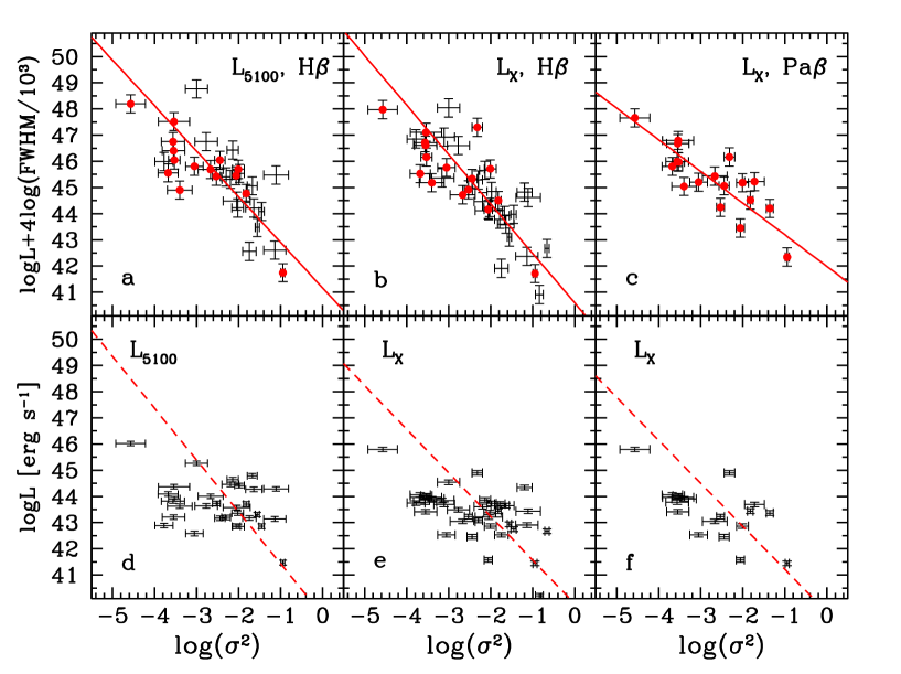
Figure 1.— (a) Square of the virial product (computed using L₅₁₀₀ and FWHM_Hβ) as a function of the excess variance, $\sigma^{2}_{\rm rms}$, of the 2-10 keV flux measured into 20 ks long bins. The continuous lines show the fit to the data (see Table 2). The objects having the Pa$\beta$ FWHM measures available are shown by red filled circles. (b) As in the previous panel using L_X and FWHM_Hβ. (c) As in the previous panel using L_X and FWHM_Paβ. (d) L₅₁₀₀ as a function of $\sigma^{2}_{\rm rms}$ of the same sample shown in the upper panel. (e) L_X as a function of $\sigma^{2}_{\rm rms}$ of the same sample shown in the upper panel. (f) L_X as a function of $\sigma^{2}_{\rm rms}$ of the same sample shown in the upper panel. The dashed lines show the best fits to the data (see Table 2).

A correlation between the AGN luminosity and the X-ray variability (without using the line width of a BLR line as a second parameter) of the type

$${\rm log}{\rm L\over{\rm erg~{}s^{-1}}}=\alpha^{\prime}\cdot{\rm log}\sigma^{2}_{\rm rms}+\beta^{\prime},$$ (8)

was already reported (e.g. Ponti et al., 2012, and references therein). If the same sample is used, the linear correlation between logL₅₁₀₀ and log$\sigma^{2}_{\rm rms}$has a spread of 1.78 dex (instead of 1.12 dex) while the correlation coefficient is -0.36 instead of -0.73 (see Figure 1 and Table 2). It is then evident that the virial product is significantly better correlated with the AGN variability than the luminosity alone.

Slightly better results are obtained if the intrinsic 2-10 keV luminosity, L_X, instead of the optical luminosity, L₅₁₀₀, is used to compute the virial product. In this case the total and intrinsic spreads are 1.06 dex and 0.93 dex, respectively (see Figure 1 and Table 2). Also in this case the virial product is better correlated with $\sigma^{2}_{\rm rms}$ (r=-0.81 and probability $5\times 10^{-10}$) than L_X alone is (r=-0.57 and spread 1.36 dex).

Finally, if the virial product is computed using L_X and Pa$\beta$, the spreads considerably decrease down to 0.71 dex (total) and 0.56 dex (intrinsic), while the correlation coefficient results to be r$=-0.82$ with a probability of $3\times 10^{-5}$ (see Table 2 and Figure 1). The correlation between L_X only and $\sigma^{2}_{\rm rms}$ has instead a less significant coefficient r$=-0.63$ (probability $4\times 10^{-3}$) and a larger spread of 1.33 dex.

Table 2Parameters of the fits

Variables	$\alpha$	$\beta$	N. Obj	r	Prob(r)	Spread	Intrinsic Spread
						dex	dex
(1)	(2)	(3)	(4)	(5)	(6)	(7)	(8)
L5100, Hβ	-1.74$\pm$0.13	41.17$\pm$0.29	31	-0.734	3$\times 10^{-6}$	1.12	1.00
L5100	-1.98$\pm$0.11	39.45$\pm$0.20	31	-0.363	5$\times 10^{-2}$	1.78	1.72
LX, Hβ	-1.89$\pm$0.10	40.59$\pm$0.23	38	-0.813	5$\times 10^{-10}$	1.06	0.93
LX	-1.67$\pm$0.07	39.90$\pm$0.12	38	-0.570	2$\times 10^{-4}$	1.36	1.32
LX, Paβ	-1.21$\pm$0.12	41.99$\pm$0.31	18	-0.822	3$\times 10^{-5}$	0.71	0.56
LX	-1.64$\pm$0.09	39.58$\pm$0.18	18	-0.634	5$\times 10^{-3}$	1.33	1.28

Note. — Column 1: variables used to compute either the virial product or the luminosity. Columns 2 and 3: best fit parameters of eq. 7. Column 4: number of objects used. Column 5: correlation coefficient. Column 6: probability of the correlation coefficient. Column 7: logarithmic spread of the data on the y axis. Column 8: intrinsic logarithmic spread of the data on the y axis.

5. Discussion and Conclusions

The above described fits show that, as expected, highly significant relationships exist between the virial products and the AGN X-ray flux variability. These relationships allow us to predict the AGN 2-10 keV luminosities. The less scattered relation has a spread of 0.6-0.7 dex and is obtained when the Pa$\beta$ line width is used. This could be due either because the Pa$\beta$ broad emission line, contrary to H$\beta$, is observed to be practically unblended with other chemical species, or because, as our analysis is based on a collection of data from public archives, the Pa$\beta$ line widths, which comes from the same project (Landt et al., 2008, 2013), could have therefore been measured in a more homogeneous way. In this case, it is then probable that new dedicated homogeneous observing programs could obtain even less scattered calibrations; at least for the H$\beta$-based relationships discussed in this work.

In order to use this method to measure the cosmological distances and then the curvature of the Universe, it is necessary to obtain reliable variability measures, corrected for the cosmological time-dilation, at relevant redshifts. In this respect, the relations based on the H$\beta$ line width measurement are the most promising as can be used even up to redshift $\sim$3 via near infra-red spectroscopic observations (e.g. in the 1-5 $\mu m$ wavelength range with NIRSpec on the James Webb Space Telescope). Moreover, recent studies by Lanzuisi et al. (2014) suggest that previous claims of a dependence on redshift of the AGN X-ray variability should be attributed to selection effects.

Our AGN-based relations constitute a distance indicator alternative to SNeIa and GRB, that can be used to cross-check their distance estimates, revealing potential unknown sources of systematic errors in their calibration and improve the constraints on fundamental cosmological parameters including dark energy properties. To assess cosmological relevance of our distance estimate we compare, in Figure 2, the luminosity distance, D_L, of our estimator (blue dots) with two different sets of cosmological models. The first one refers to flat $\Lambda$CDM models allowed by the Union2.1 compilation of SNeIa (Suzuki et al., 2012). The black curve represents the best fit, while the red dashed and dotted curves are the $\pm 1\sigma$ bounds. The corresponding values for $\Omega_{\rm M}$ are indicated in the plot. The second sets of curves represent a flat Dark Energy models with a non-evolving equation of state ($w$CDM), i.e. with constant $w$-parameter ($w\equiv p/\rho$), consistent with both the Planck maps and galaxy clustering in the BOSS survey (Sánchez et al., 2013), but with no reference to SNeIa data. The two blue dot-dashed and dashed curves represent $\pm 1\sigma$ bounds with cosmological parameters indicated in the plot.

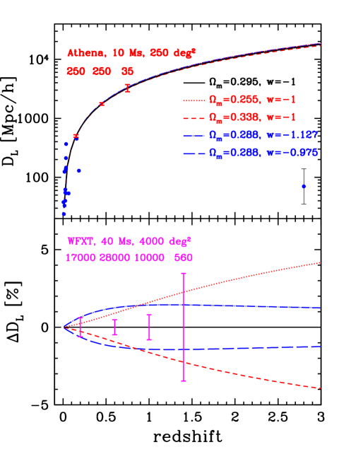
Figure 2.— Top. Luminosity distance as a function of redshift. The curves represent cosmological models allowed by different datasets described in the text. Our measures, using L_X and Pa$\beta$, are shown by blue dots. On the lower right corner the typical uncertainty on a single measurement is shown. Red error bars show the expected uncertainties from a survey carried out with Athena. The expected number of AGNs in each of the 0.4-wide redshift bins is also shown. Bottom. Percent differences of the various cosmological models compared to their respective best fit. Magenta error bars show the expected uncertainties from a survey carried out with a future WFXT as described in the text. The expected number of AGNs in each of the 0.3-wide redshift bins is also shown.

From a cosmological viewpoint our present application should be considered as a proof of concept that, however, can be developed by future missions such as the new mission concept Athena (recently proposed to the European Space Agency; Nandra et al., 2013). As D_L is proportional to the square root of the luminosity, the 0.7 dex uncertainty on the prediction of the AGN X-ray luminosity corresponds to a 0.35 dex uncertainty on the D_L measurement (see lower right corner in the upper panel of Figure 2). This implies that, if log-normal errors are assumed, variability measures of samples containing a number of AGN, N_AGN, all having similar redshifts, will provide measures of the distance (at that average redshift) with uncertainties of $\sim$0.35/$\sqrt{\rm N_{\rm AGN}}$ dex. From Vaughan et al. (2003), in low signal-to-noise measurement conditions (when the Poissonian noise dominates), the excess variance measurement is larger than the noise when

$$\sigma^{2}_{\rm rms}>\sqrt{2\over\rm N}{1\over{\mu t_{o}}},$$ (9)

where N is the number of $t_{o}$ long time intervals, and $\mu$ is the average count rate in $ph/s$ units. As also confirmed by our data, the above formula requires a count rate $\mu\sim 1~{}ph/s$ and 80 bins, $t_{o}=250$ s long, in order to measure $\sigma^{2}_{\rm rms}$ larger than $\sim 5\times 10^{-4}$ (as mainly observed in this work). If Athena will be used, $\mu\sim 1~{}ph/s$ corresponds to a 2-10 keV flux of 10^-13 erg s^-1 cm^-2. According to the AGN X-ray luminosity function (La Franca et al., 2005; Gilli et al., 2007), at these fluxes, with a 10 Ms survey covering 250 deg² with 500 pointings of the Wide Field Instrument ($\sim$0.5 deg² large field of view), it will be possible to measure $\sigma^{2}_{\rm rms}$  in a sample of $\sim$250 unabsorbed (N${}_{\rm H}<$10²¹ cm^-2) AGN contained in each of the redshifts bins 0$<z<$0.3 and 0.3$<z<$0.6, and a sample of $\sim$35 AGN in the redshift bin 0.6$<z<$0.9. In this case D_L could be measured with a 0.02 dex uncertainty (0.1 mag) at redshifts less than 0.6, and with a 0.06 dex (0.3 mag) uncertainty in the 0.6$<z<$0.9 bin (red error-bars in Figure 2). With the proposed Athena survey our estimator will not be competitive with SNeIa. It will, however, provide a cosmological test independent from SNeIa able to detect possible systematic errors if larger than 0.1 mag in the redshift range $z<0.6$. A value a factor of $\sim 4$ more precise than the other alternative estimator based on the GRBs (Schaefer, 2007).

In order to significantly exploit at higher redshifts our proposed $\sigma^{2}_{\rm rms}$-based AGN luminosity indicator to constraint the Universe geometry a further step is necessary, such as a dedicated Wide Field X-ray Telescope (WFXT) with an effective collecting area at least three times larger than Athena and $\sim$2 deg² large field of view. In this case, as an example, with a 40 Ms long program it would be possible to measure D_L with less than 0.003 dex (0.015 mag) uncertainties at redshift below 1.2 and an uncertainty of less than 0.02 dex (0.1 mag) in the redshift range $1.2<z<1.6$. The bottom panel of Figure 2 illustrates more clearly the potential of our new estimator. The curves represent the per cent difference of the luminosity distance models shown in the upper panel with respect to its reference best fit scenario. From the comparison between the magenta error-bars with the model scatter, we conclude that our estimator has the prospect to become a cosmological probe even more sensitive than current SNeIa if applied to AGN samples as large as that of an hypothetical future survey carried out with a dedicated WFXT as described above.

References

- Assef et al. (2012) Assef, R. J., Frank, S., Grier, C. J., et al. 2012, ApJ, 753, L2
- Baldwin (1977) Baldwin, J. A. 1977, ApJ, 214, 679
- Bentz et al. (2013) Bentz, M. C., Denney, K. D., Grier, C. J., et al. 2013, ApJ, 767, 149
- Boller et al. (1996) Boller, T., Brandt, W. N., & Fink, H. 1996, A&A, 305, 53
- Collier et al. (1999) Collier, S., Horne, K., Wanders, I., & Peterson, B. M. 1999, MNRAS, 302, L24
- Conconi et al. (2010) Conconi, P., Campana, S., Tagliaferri, G., et al. 2010, MNRAS, 405, 877
- Denney et al. (2009) Denney, K. D., Peterson, B. M., Dietrich, M., Vestergaard, M., & Bentz, M. C. 2009, ApJ, 692, 246
- Elvis & Karovska (2002) Elvis, M., & Karovska, M. 2002, ApJ, 581, L67
- Gierliński et al. (2008) Gierliński, M., Nikołajuk, M., & Czerny, B. 2008, MNRAS, 383, 741
- Gilli et al. (2007) Gilli, R., Comastri, A., & Hasinger, G. 2007, A&A, 463, 79
- Grupe et al. (1999) Grupe, D., Beuermann, K., Mannheim, K., & Thomas, H.-C. 1999, A&A, 350, 805
- Grupe et al. (2004) Grupe, D., Wills, B. J., Leighly, K. M., & Meusinger, H. 2004, AJ, 127, 156
- Jin et al. (2012) Jin, C., Ward, M., Done, C., & Gelbord, J. 2012, MNRAS, 420, 1825
- Kelly et al. (2013) Kelly, B. C., Treu, T., Malkan, M., Pancoast, A., & Woo, J.-H. 2013, ApJ, 779, 187
- Kraemer et al. (1999) Kraemer, S. B., Turner, T. J., Crenshaw, D. M., & George, I. M. 1999, ApJ, 519, 69
- La Franca et al. (2005) La Franca, F., Fiore, F., Comastri, A., et al. 2005, ApJ, 635, 864
- Landt et al. (2008) Landt, H., Bentz, M. C., Ward, M. J., et al. 2008, ApJS, 174, 282
- Landt et al. (2013) Landt, H., Ward, M. J., Peterson, B. M., et al. 2013, MNRAS, 432, 113
- Lanzuisi et al. (2014) Lanzuisi, G., Ponti, G., Salvato, M., et al. 2014, ApJ, 781, 105
- Leighly (1999) Leighly, K. M. 1999, ApJS, 125, 317
- Marziani & Sulentic (2013) Marziani, P., & Sulentic, J. W. 2013, arXiv:1310.3143
- McHardy et al. (2005) McHardy, I. M., Gunn, K. F., Uttley, P., & Goad, M. R. 2005, MNRAS, 359, 1469
- McHardy et al. (2006) McHardy, I. M., Koerding, E., Knigge, C., Uttley, P., & Fender, R. P. 2006, Nature, 444, 730
- McLure & Dunlop (2001) McLure, R. J., & Dunlop, J. S. 2001, MNRAS, 327, 199
- McLure & Jarvis (2002) McLure, R. J., & Jarvis, M. J. 2002, MNRAS, 337, 109
- Nandra et al. (1997) Nandra, K., Mushotzky, R. F., Yaqoob, T., George, I. M., & Turner, T. J. 1997, MNRAS, 284, L7
- Nandra et al. (2013) Nandra, K., Barret, D., Barcons, X., et al. 2013, ArXiv e-prints, arXiv:1306.2307
- O’Neill et al. (2005) O’Neill, P. M., Nandra, K., Papadakis, I. E., & Turner, T. J. 2005, MNRAS, 358, 1405
- Perlmutter et al. (1999) Perlmutter, S., Aldering, G., Goldhaber, G., et al. 1999, ApJ, 517, 565
- Ponti et al. (2012) Ponti, G., Papadakis, I., Bianchi, S., et al. 2012, A&A, 542, A83
- Press et al. (2007) Press, W. H., Teukolsky, S. A., Vetterling, W. T., & Flannery, B. P. 2007, Numerical recipes: the art of scientific computing, 3rd edn. (Cambridge Univ. Press, Cambridge)
- Riess et al. (1998) Riess, A. G., Filippenko, A. V., Challis, P., et al. 1998, AJ, 116, 1009
- Rubin et al. (2013) Rubin, D., Knop, R. A., Rykoff, E., et al. 2013, ApJ, 763, 35
- Rudge & Raine (1999) Rudge, C. M., & Raine, D. J. 1999, MNRAS, 308, 1150
- Sánchez et al. (2013) Sánchez, A. G., Kazin, E. A., Beutler, F., et al. 2013, MNRAS, 433, 1202
- Schaefer (2007) Schaefer, B. E. 2007, ApJ, 660, 16
- Shemmer et al. (2014) Shemmer, O., Brandt, W. N., Paolillo, M., et al. 2014, ArXiv e-prints, arXiv:1401.5496
- Suzuki et al. (2012) Suzuki, N., Rubin, D., Lidman, C., et al. 2012, ApJ, 746, 85
- Torres et al. (1997) Torres, C. A. O., Quast, G. R., Coziol, R., et al. 1997, ApJ, 488, L19
- Turner et al. (1999) Turner, T. J., George, I. M., Nandra, K., & Turcan, D. 1999, ApJ, 524, 667
- Vaughan et al. (2003) Vaughan, S., Edelson, R., Warwick, R. S., & Uttley, P. 2003, MNRAS, 345, 1271
- Vestergaard & Osmer (2009) Vestergaard, M., & Osmer, P. S. 2009, ApJ, 699, 800
- Vestergaard & Peterson (2006) Vestergaard, M., & Peterson, B. M. 2006, ApJ, 641, 689
- Wandel et al. (1999) Wandel, A., Peterson, B. M., & Malkan, M. A. 1999, ApJ, 526, 579
- Wang et al. (2013) Wang, J.-M., Du, P., Valls-Gabaud, D., Hu, C., & Netzer, H. 2013, Physical Review Letters, 110, 081301
- Watson et al. (2011) Watson, D., Denney, K. D., Vestergaard, M., & Davis, T. M. 2011, ApJ, 740, L49
- Winkler (1992) Winkler, H. 1992, MNRAS, 257, 677
- Zhou et al. (2006) Zhou, H., Wang, T., Yuan, W., et al. 2006, ApJS, 166, 128
- Zhou et al. (2010) Zhou, X.-L., Zhang, S.-N., Wang, D.-X., & Zhu, L. 2010, ApJ, 710, 16