1. Introduction
For a hypersurface Ω 0 subscript Ω 0 \Omega_{0} 𝑿 ~ 0 : M n → ℝ n + 1 : subscript ~ 𝑿 0 → superscript 𝑀 𝑛 superscript ℝ 𝑛 1 \tilde{\bm{X}}_{0}:M^{n}\rightarrow\mathbb{R}^{n+1} M n superscript 𝑀 𝑛 M^{n} n 𝑛 n { Ω t : t ∈ [ 0 , T ) } conditional-set subscript Ω 𝑡 𝑡 0 𝑇 \left\{\Omega_{t}:t\in[0,T)\right\} T > 0 𝑇 0 T>0 Ω t = 𝑿 ( M n , t ) subscript Ω 𝑡 𝑿 superscript 𝑀 𝑛 𝑡 \Omega_{t}=\bm{X}\left(M^{n},t\right) 𝑿 𝑿 \bm{X}
(1) ∂ 𝑿 ∂ t = ( 1 ∫ M n Ξ ( 𝜿 ) 𝑑 μ t ∫ M n F ( 𝜿 ) Ξ ( 𝜿 ) 𝑑 μ t − F ( 𝜿 ) ) 𝝂 , 𝑿 ( ⋅ , 0 ) = 𝑿 ~ 0 , formulae-sequence 𝑿 𝑡 1 subscript superscript 𝑀 𝑛 Ξ 𝜿 differential-d subscript 𝜇 𝑡 subscript superscript 𝑀 𝑛 𝐹 𝜿 Ξ 𝜿 differential-d subscript 𝜇 𝑡 𝐹 𝜿 𝝂 𝑿 ⋅ 0 subscript ~ 𝑿 0 \frac{\partial\bm{X}}{\partial t}=\left(\frac{1}{\int_{M^{n}}\Xi\left(\bm{\kappa}\right)\,d\mu_{t}}\int_{M^{n}}F\left(\bm{\kappa}\right)\Xi\left(\bm{\kappa}\right)\,d\mu_{t}-F\left(\bm{\kappa}\right)\right)\bm{\nu},\ \ \bm{X}\left(\cdot,0\right)=\tilde{\bm{X}}_{0},
where F ( 𝜿 ) 𝐹 𝜿 F\left(\bm{\kappa}\right) Ξ ( 𝜿 ) Ξ 𝜿 \Xi\left(\bm{\kappa}\right) 𝜿 = ( κ 1 , … , κ n ) 𝜿 subscript 𝜅 1 … subscript 𝜅 𝑛 \bm{\kappa}=(\kappa_{1},\ldots,\kappa_{n}) 𝝂 𝝂 \bm{\nu} d μ t 𝑑 subscript 𝜇 𝑡 \,d\mu_{t} Ω t subscript Ω 𝑡 \Omega_{t} (A1) -(A3) below, was proved in [9 ] .
This flow is a generalisation of the volume preserving mean curvature flow (VPMCF), which has F ( 𝜿 ) = ∑ a = 1 n κ a 𝐹 𝜿 superscript subscript 𝑎 1 𝑛 subscript 𝜅 𝑎 F\left(\bm{\kappa}\right)=\sum_{a=1}^{n}\kappa_{a} Ξ ( 𝜿 ) = 1 Ξ 𝜿 1 \Xi(\bm{\kappa})=1 Ω t subscript Ω 𝑡 \Omega_{t} Ω 0 subscript Ω 0 \Omega_{0} t → ∞ → 𝑡 t\rightarrow\infty [5 , 11 ] . The stability of spheres as stationary solutions to the VPMCF has previously been studied by Escher and Simonett. In [4 ] Escher and Simonett consider graphs over spheres and prove that if the height function is small in the little-Hölder space h 1 , β superscript ℎ 1 𝛽
h^{1,\beta} [2 ] , where convergence to a sphere was obtained for convex hypersurfaces under an additional pinching assumption. When the weight function is an elementary symmetric function the flow is the mixed-volume preserving curvature flow, which has been studied by McCoy in [15 ] for speed functions given by the mean curvature and in [16 ] for a more general class of speed functions. In both cases it was proved that if the initial hypersurface is strictly convex it will converge to a sphere under the flow.
In the present article we consider the setting introduced by Athanassenas in [1 ] . That is, we consider hypersurfaces, Ω Ω \Omega
W = { 𝒙 ∈ ℝ n + 1 : 0 < x n + 1 < d } , d > 0 , formulae-sequence 𝑊 conditional-set 𝒙 superscript ℝ 𝑛 1 0 subscript 𝑥 𝑛 1 𝑑 𝑑 0 W=\left\{\bm{x}\in\mathbb{R}^{n+1}:0<x_{n+1}<d\right\},\ d>0,
such that ∂ Ω ⊂ ∂ W Ω 𝑊 \partial\Omega\subset\partial W Ω Ω \Omega ∂ W 𝑊 \partial W V o l 𝑉 𝑜 𝑙 Vol Ω 0 subscript Ω 0 \Omega_{0} ∂ W 𝑊 \partial W
(2) | Ω 0 | := ∫ M n 𝑑 μ 0 ≤ V o l d , assign subscript Ω 0 subscript superscript 𝑀 𝑛 differential-d subscript 𝜇 0 𝑉 𝑜 𝑙 𝑑 \left|\Omega_{0}\right|:=\int_{M^{n}}\,d\mu_{0}\leq\frac{Vol}{d},
then the VPMCF will exist for all time and the hypersurfaces will converge to a cylinder. In this case the assumption (2 Ω t subscript Ω 𝑡 \Omega_{t} [8 ] the author considered graphs over cylinders and proved that a cylinder of radius
R > d n − 1 π , 𝑅 𝑑 𝑛 1 𝜋 R>\frac{d\sqrt{n-1}}{\pi},
is stable under the VPMCF, in the same sense as in [4 ] . In [9 ] this result was extended to the flow (1
(3) R > d π ( n − 1 ) ∂ F ∂ κ 1 ( 𝜿 R ) ∂ F ∂ κ n ( 𝜿 R ) , 𝑅 𝑑 𝜋 𝑛 1 𝐹 subscript 𝜅 1 subscript 𝜿 𝑅 𝐹 subscript 𝜅 𝑛 subscript 𝜿 𝑅 R>\frac{d}{\pi}\sqrt{\frac{(n-1)\frac{\partial F}{\partial\kappa_{1}}\left(\bm{\kappa}_{R}\right)}{\frac{\partial F}{\partial\kappa_{n}}\left(\bm{\kappa}_{R}\right)}},
where 𝜿 R = ( 1 R , … , 1 R , 0 ) subscript 𝜿 𝑅 1 𝑅 … 1 𝑅 0 \bm{\kappa}_{R}=\left(\frac{1}{R},\ldots,\frac{1}{R},0\right)
Theorem 1.1 ([9 ] ).
Let 𝒞 R , d n superscript subscript 𝒞 𝑅 𝑑
𝑛 \mathscr{C}_{R,d}^{n} R 𝑅 R d 𝑑 d (A1) -(A3) are satisfied for R ~ = R ~ 𝑅 𝑅 \tilde{R}=R O c ⊂ h ∂ ∂ z 2 , α ( 𝒞 ¯ R , d n ) subscript 𝑂 𝑐 subscript superscript ℎ 2 𝛼
𝑧 superscript subscript ¯ 𝒞 𝑅 𝑑
𝑛 O_{c}\subset h^{2,\alpha}_{\frac{\partial}{\partial z}}\left(\overline{\mathscr{C}}_{R,d}^{n}\right) 0 < α < 1 0 𝛼 1 0<\alpha<1 2 Ω 0 subscript Ω 0 \Omega_{0} 𝒞 R , d n superscript subscript 𝒞 𝑅 𝑑
𝑛 \mathscr{C}_{R,d}^{n} O c subscript 𝑂 𝑐 O_{c} T > 0 𝑇 0 T>0 1 t ∈ [ 0 , T ) 𝑡 0 𝑇 t\in[0,T) 3 T = ∞ 𝑇 T=\infty t → ∞ → 𝑡 t\rightarrow\infty h 2 , α ( 𝒞 ¯ R , d n ) superscript ℎ 2 𝛼
superscript subscript ¯ 𝒞 𝑅 𝑑
𝑛 h^{2,\alpha}\left(\overline{\mathscr{C}}_{R,d}^{n}\right)
It is important to note that in general both sides of (3 R 𝑅 R 𝜿 𝜿 \bm{\kappa} 3 R 𝑅 R [13 ] . In that paper LeCrone also showed that the cylinder of radius d π 𝑑 𝜋 \frac{d}{\pi}
For the main analysis we make some assumptions on the form of F 𝐹 F Ξ Ξ \Xi
(A1):
F 𝐹 F Ξ Ξ \Xi
(A2):
∂ F ∂ κ a ( 𝜿 R ~ ) > 0 𝐹 subscript 𝜅 𝑎 subscript 𝜿 ~ 𝑅 0 \frac{\partial F}{\partial\kappa_{a}}\left(\bm{\kappa}_{\tilde{R}}\right)>0 a = 1 , … , n 𝑎 1 … 𝑛
a=1,\ldots,n R ~ ∈ ℝ + ~ 𝑅 superscript ℝ \tilde{R}\in\mathbb{R}^{+}
(A3):
Ξ ( 𝜿 R ~ ) > 0 Ξ subscript 𝜿 ~ 𝑅 0 \Xi\left(\bm{\kappa}_{\tilde{R}}\right)>0 R ~ ∈ ℝ + ~ 𝑅 superscript ℝ \tilde{R}\in\mathbb{R}^{+}
(A4):
Ξ ( 𝜿 ) = ∑ a = 0 n c a E a ( 𝜿 ) Ξ 𝜿 superscript subscript 𝑎 0 𝑛 subscript 𝑐 𝑎 subscript 𝐸 𝑎 𝜿 \Xi(\bm{\kappa})=\sum_{a=0}^{n}c_{a}E_{a}(\bm{\kappa})
(A5):
There exists R c r i t > 0 subscript 𝑅 𝑐 𝑟 𝑖 𝑡 0 R_{crit}>0 R c r i t subscript 𝑅 𝑐 𝑟 𝑖 𝑡 R_{crit} 3 R > R c r i t 𝑅 subscript 𝑅 𝑐 𝑟 𝑖 𝑡 R>R_{crit} R < R c r i t 𝑅 subscript 𝑅 𝑐 𝑟 𝑖 𝑡 R<R_{crit} R < R c r i t 𝑅 subscript 𝑅 𝑐 𝑟 𝑖 𝑡 R<R_{crit} R > R c r i t 𝑅 subscript 𝑅 𝑐 𝑟 𝑖 𝑡 R>R_{crit}
where
(4) E a ( 𝜿 ) = ∑ 1 ≤ b 1 < … < b a ≤ n ∏ i = 1 a κ b i , subscript 𝐸 𝑎 𝜿 subscript 1 subscript 𝑏 1 … subscript 𝑏 𝑎 𝑛 superscript subscript product 𝑖 1 𝑎 subscript 𝜅 subscript 𝑏 𝑖 E_{a}\left(\bm{\kappa}\right)=\sum_{1\leq b_{1}<\ldots<b_{a}\leq n}\prod_{i=1}^{a}\kappa_{b_{i}},
are the elementary symmetric functions. The first two assumptions ensure isotropy and local parabolicity respectively, while (A3) ensures a valid flow. Assumption (A4) ensures that a type of weighted-volume is preserved under the flow, see Appendix A (A5) is not the most descriptive assumption, we note here that it is satisfied when F 𝐹 F
(A5)*:
F 𝐹 F k 𝑘 k F ( α 𝜿 ) = α k F ( 𝜿 ) 𝐹 𝛼 𝜿 superscript 𝛼 𝑘 𝐹 𝜿 F(\alpha\bm{\kappa})=\alpha^{k}F(\bm{\kappa}) α > 0 𝛼 0 \alpha>0
We note that when this assumption is used, we have R c r i t = d π ( n − 1 ) ∂ F ∂ κ 1 ( 𝜿 1 ) ∂ F ∂ κ n ( 𝜿 1 ) subscript 𝑅 𝑐 𝑟 𝑖 𝑡 𝑑 𝜋 𝑛 1 𝐹 subscript 𝜅 1 subscript 𝜿 1 𝐹 subscript 𝜅 𝑛 subscript 𝜿 1 R_{crit}=\frac{d}{\pi}\sqrt{\frac{(n-1)\frac{\partial F}{\partial\kappa_{1}}\left(\bm{\kappa}_{1}\right)}{\frac{\partial F}{\partial\kappa_{n}}\left(\bm{\kappa}_{1}\right)}} (A2) is true for some R ~ > 0 ~ 𝑅 0 \tilde{R}>0 R ~ > 0 ~ 𝑅 0 \tilde{R}>0
Theorem 1.2 .
For the flow (1 (A1) -(A5) satisfied for R ~ = R c r i t ~ 𝑅 subscript 𝑅 𝑐 𝑟 𝑖 𝑡 \tilde{R}=R_{crit} R c r i t subscript 𝑅 𝑐 𝑟 𝑖 𝑡 R_{crit} 44
In (44 F a ( η ) = ∂ F ∂ κ a ( 𝜿 n − 1 η ) subscript 𝐹 𝑎 𝜂 𝐹 subscript 𝜅 𝑎 subscript 𝜿 𝑛 1 𝜂 F_{a}(\eta)=\frac{\partial F}{\partial\kappa_{a}}\left(\bm{\kappa}_{\frac{n-1}{\eta}}\right) a = { 1 , n } 𝑎 1 𝑛 a=\{1,n\} F n n ( η ) = ∂ 2 F ∂ κ n 2 ( 𝜿 n − 1 η ) subscript 𝐹 𝑛 𝑛 𝜂 superscript 2 𝐹 superscript subscript 𝜅 𝑛 2 subscript 𝜿 𝑛 1 𝜂 F_{nn}(\eta)=\frac{\partial^{2}F}{\partial\kappa_{n}^{2}}\left(\bm{\kappa}_{\frac{n-1}{\eta}}\right) F n n n ( η ) = ∂ 3 F ∂ κ n 3 ( 𝜿 n − 1 η ) subscript 𝐹 𝑛 𝑛 𝑛 𝜂 superscript 3 𝐹 superscript subscript 𝜅 𝑛 3 subscript 𝜿 𝑛 1 𝜂 F_{nnn}(\eta)=\frac{\partial^{3}F}{\partial\kappa_{n}^{3}}\left(\bm{\kappa}_{\frac{n-1}{\eta}}\right) (A5)* is satisfied then these functions are homogeneous, so have the representations F a ( η ) = η k − 1 F a subscript 𝐹 𝑎 𝜂 superscript 𝜂 𝑘 1 subscript 𝐹 𝑎 F_{a}(\eta)=\eta^{k-1}F_{a} F n n ( η ) = η k − 2 F n n subscript 𝐹 𝑛 𝑛 𝜂 superscript 𝜂 𝑘 2 subscript 𝐹 𝑛 𝑛 F_{nn}(\eta)=\eta^{k-2}F_{nn} F n n n ( η ) = η k − 3 F n n n subscript 𝐹 𝑛 𝑛 𝑛 𝜂 superscript 𝜂 𝑘 3 subscript 𝐹 𝑛 𝑛 𝑛 F_{nnn}(\eta)=\eta^{k-3}F_{nnn} F a := F a ( 1 ) assign subscript 𝐹 𝑎 subscript 𝐹 𝑎 1 F_{a}:=F_{a}(1) F n n := F n n ( 1 ) assign subscript 𝐹 𝑛 𝑛 subscript 𝐹 𝑛 𝑛 1 F_{nn}:=F_{nn}(1) F n n n := F n n n ( 1 ) assign subscript 𝐹 𝑛 𝑛 𝑛 subscript 𝐹 𝑛 𝑛 𝑛 1 F_{nnn}:=F_{nnn}(1)
Corollary 1.4 .
For the flow (1 (A1) - (A5)* satisfied for R ~ = d m π ( n − 1 ) F 1 F n ~ 𝑅 𝑑 𝑚 𝜋 𝑛 1 subscript 𝐹 1 subscript 𝐹 𝑛 \tilde{R}=\frac{d}{m\pi}\sqrt{\frac{(n-1)F_{1}}{F_{n}}} m ∈ ℕ 𝑚 ℕ m\in\mathbb{N} d m π ( n − 1 ) F 1 F n 𝑑 𝑚 𝜋 𝑛 1 subscript 𝐹 1 subscript 𝐹 𝑛 \frac{d}{m\pi}\sqrt{\frac{(n-1)F_{1}}{F_{n}}} m = 1 𝑚 1 m=1
(5) − 6 ( n − 1 ) ∑ a = 1 n c a π a d a ( F n ( n − 1 ) F 1 ) a 2 ( ( n − 2 a − 1 ) − F 1 F n ( n − 1 a − 1 ) ) ∑ a = 0 n c a π a d a ( F n ( n − 1 ) F 1 ) a 2 ( n − 1 a ) − k 2 + 6 n + 6 − 3 F 1 2 F n n n 2 F n 3 6 𝑛 1 superscript subscript 𝑎 1 𝑛 subscript 𝑐 𝑎 superscript 𝜋 𝑎 superscript 𝑑 𝑎 superscript subscript 𝐹 𝑛 𝑛 1 subscript 𝐹 1 𝑎 2 binomial 𝑛 2 𝑎 1 subscript 𝐹 1 subscript 𝐹 𝑛 binomial 𝑛 1 𝑎 1 superscript subscript 𝑎 0 𝑛 subscript 𝑐 𝑎 superscript 𝜋 𝑎 superscript 𝑑 𝑎 superscript subscript 𝐹 𝑛 𝑛 1 subscript 𝐹 1 𝑎 2 binomial 𝑛 1 𝑎 superscript 𝑘 2 6 𝑛 6 3 superscript subscript 𝐹 1 2 subscript 𝐹 𝑛 𝑛 𝑛 2 superscript subscript 𝐹 𝑛 3 \displaystyle\frac{-6(n-1)\sum_{a=1}^{n}\frac{c_{a}\pi^{a}}{d^{a}}\left(\frac{F_{n}}{(n-1)F_{1}}\right)^{\frac{a}{2}}\left(\binom{n-2}{a-1}-\frac{F_{1}}{F_{n}}\binom{n-1}{a-1}\right)}{\sum_{a=0}^{n}\frac{c_{a}\pi^{a}}{d^{a}}\left(\frac{F_{n}}{(n-1)F_{1}}\right)^{\frac{a}{2}}\binom{n-1}{a}}-k^{2}+6n+6-\frac{3F_{1}^{2}F_{nnn}}{2F_{n}^{3}}
+ 2 F 1 2 F n n 2 F n 4 + k F 1 F n n 2 F n + ( n − 1 ) F 1 2 F n n F n 3 − ( n − 1 ) 2 F 1 2 F n 2 − ( n − 1 ) ( k − 3 ) F 1 F n < 0 , 2 superscript subscript 𝐹 1 2 superscript subscript 𝐹 𝑛 𝑛 2 superscript subscript 𝐹 𝑛 4 𝑘 subscript 𝐹 1 subscript 𝐹 𝑛 𝑛 2 subscript 𝐹 𝑛 𝑛 1 superscript subscript 𝐹 1 2 subscript 𝐹 𝑛 𝑛 superscript subscript 𝐹 𝑛 3 superscript 𝑛 1 2 superscript subscript 𝐹 1 2 superscript subscript 𝐹 𝑛 2 𝑛 1 𝑘 3 subscript 𝐹 1 subscript 𝐹 𝑛 0 \displaystyle\hskip 17.07182pt+\frac{2F_{1}^{2}F_{nn}^{2}}{F_{n}^{4}}+\frac{kF_{1}F_{nn}}{2F_{n}}+\frac{(n-1)F_{1}^{2}F_{nn}}{F_{n}^{3}}-\frac{(n-1)^{2}F_{1}^{2}}{F_{n}^{2}}-\frac{(n-1)(k-3)F_{1}}{F_{n}}<0,
holds, then the stationary solutions close to the cylinder of radius d π ( n − 1 ) F 1 F n 𝑑 𝜋 𝑛 1 subscript 𝐹 1 subscript 𝐹 𝑛 \frac{d}{\pi}\sqrt{\frac{(n-1)F_{1}}{F_{n}}}
Note that the first result of this Corollary is slightly stronger than what is immediately obtained from Theorem 1.2 3.3 1.4 1.2 F a ( η ) subscript 𝐹 𝑎 𝜂 F_{a}(\eta) F n n ( η ) subscript 𝐹 𝑛 𝑛 𝜂 F_{nn}(\eta) F n n n ( η ) subscript 𝐹 𝑛 𝑛 𝑛 𝜂 F_{nnn}(\eta)
Corollary 1.5 .
The cylinder of radius d n − 1 π 𝑑 𝑛 1 𝜋 \frac{d\sqrt{n-1}}{\pi} 2 ≤ n ≤ 10 2 𝑛 10 2\leq n\leq 10 n ≥ 11 𝑛 11 n\geq 11
In Section 2 d π 𝑑 𝜋 \frac{d}{\pi} 3 1.2 4 1.5 5 [10 ] . This is then used to provide more insight into the results of Section 4
The author is thankful to the University of Queensland and Dr Artem Pulemotov along with Monash University and Dr Maria Athanassenas for their support while preparing this paper. Part of this work was initiated during the author’s PhD candidature at Monash University.
2. Reducing the Equation
We consider normal graphs over cylinders, hence M n = 𝕊 n − 1 × ( 0 , d ) superscript 𝑀 𝑛 superscript 𝕊 𝑛 1 0 𝑑 M^{n}=\mathbb{S}^{n-1}\times(0,d)
𝑿 ρ ( 𝜽 , z ) = ( ρ ( z ) Y 1 , 1 n − 1 ( 𝜽 ) , … , ρ ( z ) Y 1 , n n − 1 ( 𝜽 ) , z ) subscript 𝑿 𝜌 𝜽 𝑧 𝜌 𝑧 subscript superscript 𝑌 𝑛 1 1 1
𝜽 … 𝜌 𝑧 subscript superscript 𝑌 𝑛 1 1 𝑛
𝜽 𝑧 \bm{X}_{\rho}\left(\bm{\theta},z\right)=\left(\rho(z)Y^{n-1}_{1,1}\left(\bm{\theta}\right),\ldots,\rho(z)Y^{n-1}_{1,n}\left(\bm{\theta}\right),z\right)
where ρ : [ 0 , d ] → ℝ + : 𝜌 → 0 𝑑 superscript ℝ \rho:[0,d]\rightarrow\mathbb{R}^{+} Y 1 , a n − 1 : 𝕊 n − 1 → ℝ : subscript superscript 𝑌 𝑛 1 1 𝑎
→ superscript 𝕊 𝑛 1 ℝ Y^{n-1}_{1,a}:\mathbb{S}^{n-1}\rightarrow\mathbb{R} 1 ≤ a ≤ n 1 𝑎 𝑛 1\leq a\leq n 𝕊 n − 1 superscript 𝕊 𝑛 1 \mathbb{S}^{n-1} d ρ d z | z = 0 , d = 0 evaluated-at 𝑑 𝜌 𝑑 𝑧 𝑧 0 𝑑
0 \left.\frac{d\rho}{dz}\right|_{z=0,d}=0 1 ρ : [ 0 , d ] × [ 0 , T ) → ℝ + : 𝜌 → 0 𝑑 0 𝑇 superscript ℝ \rho:[0,d]\times[0,T)\rightarrow\mathbb{R}^{+}
(6) ∂ ρ ∂ t = 1 + ( ∂ ρ ∂ z ) 2 ( 1 ∫ [ 0 , d ] Ξ ( 𝜿 ρ ) 𝑑 μ ρ ∫ [ 0 , d ] F ( 𝜿 ρ ) Ξ ( 𝜿 ρ ) 𝑑 μ ρ − F ( 𝜿 ρ ) ) , ∂ ρ ∂ z | z = 0 , d = 0 , ρ ( ⋅ , 0 ) = ρ 0 , 𝜌 𝑡 1 superscript 𝜌 𝑧 2 1 subscript 0 𝑑 Ξ subscript 𝜿 𝜌 differential-d subscript 𝜇 𝜌 subscript 0 𝑑 𝐹 subscript 𝜿 𝜌 Ξ subscript 𝜿 𝜌 differential-d subscript 𝜇 𝜌 𝐹 subscript 𝜿 𝜌 formulae-sequence evaluated-at 𝜌 𝑧 𝑧 0 𝑑
0 𝜌 ⋅ 0 subscript 𝜌 0 \begin{array}[]{c}\frac{\partial\rho}{\partial t}=\sqrt{1+\left(\frac{\partial\rho}{\partial z}\right)^{2}}\left(\frac{1}{\int_{[0,d]}\Xi\left(\bm{\kappa}_{\rho}\right)\,d\mu_{\rho}}\int_{[0,d]}F\left(\bm{\kappa}_{\rho}\right)\Xi\left(\bm{\kappa}_{\rho}\right)\,d\mu_{\rho}-F\left(\bm{\kappa}_{\rho}\right)\right),\\
\left.\frac{\partial\rho}{\partial z}\right|_{z=0,d}=0,\hskip 19.91684pt\rho(\cdot,0)=\rho_{0},\end{array}
where 𝑿 ~ 0 = 𝑿 ρ 0 subscript ~ 𝑿 0 subscript 𝑿 subscript 𝜌 0 \tilde{\bm{X}}_{0}=\bm{X}_{\rho_{0}} d μ ρ = ρ n − 1 1 + ( ∂ ρ ∂ z ) 2 d z 𝑑 subscript 𝜇 𝜌 superscript 𝜌 𝑛 1 1 superscript 𝜌 𝑧 2 𝑑 𝑧 \,d\mu_{\rho}=\rho^{n-1}\sqrt{1+\left(\frac{\partial\rho}{\partial z}\right)^{2}}\,dz 𝜿 ρ subscript 𝜿 𝜌 \bm{\kappa}_{\rho} 𝑿 ρ subscript 𝑿 𝜌 \bm{X}_{\rho}
Throughout this paper we will be considering functions in the little-Hölder spaces, which are defined for an open set U ⊂ ℝ n 𝑈 superscript ℝ 𝑛 U\subset\mathbb{R}^{n} k ∈ ℕ 𝑘 ℕ k\in\mathbb{N} α ∈ ( 0 , 1 ) 𝛼 0 1 \alpha\in(0,1)
h 0 , α ( U ¯ ) = { f ∈ C 0 , α ( U ¯ ) : lim r → 0 sup 0 < | x − y | < r x , y ∈ U ¯ | f ( x ) − f ( y ) | | x − y | α = 0 } , superscript ℎ 0 𝛼
¯ 𝑈 conditional-set 𝑓 superscript 𝐶 0 𝛼
¯ 𝑈 subscript → 𝑟 0 subscript supremum superscript 0 𝑥 𝑦 𝑟 𝑥 𝑦
¯ 𝑈 𝑓 𝑥 𝑓 𝑦 superscript 𝑥 𝑦 𝛼 0 \displaystyle h^{0,\alpha}\left(\bar{U}\right)=\left\{f\in C^{0,\alpha}\left(\bar{U}\right):\lim_{r\rightarrow 0}\sup_{\stackrel{{\scriptstyle x,y\in\bar{U}}}{{0<|x-y|<r}}}\frac{|f(x)-f(y)|}{|x-y|^{\alpha}}=0\right\},
h k , α ( U ¯ ) = superscript ℎ 𝑘 𝛼
¯ 𝑈 absent \displaystyle h^{k,\alpha}\left(\bar{U}\right)= { f ∈ C k , α ( U ¯ ) : D β f ∈ h 0 , α ( U ¯ ) for all multi-indices β with | β | = k } , conditional-set 𝑓 superscript 𝐶 𝑘 𝛼
¯ 𝑈 superscript 𝐷 𝛽 𝑓 superscript ℎ 0 𝛼
¯ 𝑈 for all multi-indices 𝛽 with 𝛽 𝑘 \displaystyle\left\{f\in C^{k,\alpha}\left(\bar{U}\right):D^{\beta}f\in h^{0,\alpha}\left(\bar{U}\right)\text{ for all multi-indices }\beta\text{ with }|\beta|=k\right\},
where C k , α ( U ¯ ) superscript 𝐶 𝑘 𝛼
¯ 𝑈 C^{k,\alpha}\left(\bar{U}\right) ( ⋅ , ⋅ ) θ subscript ⋅ ⋅ 𝜃 (\cdot,\cdot)_{\theta} θ ∈ ( 0 , 1 ) 𝜃 0 1 \theta\in(0,1) [14 ] . That is, for k , l ∈ ℕ 𝑘 𝑙
ℕ k,l\in\mathbb{N} α , β ∈ ( 0 , 1 ) 𝛼 𝛽
0 1 \alpha,\beta\in(0,1) k + α > l + β 𝑘 𝛼 𝑙 𝛽 k+\alpha>l+\beta
(7) ( h l , β , h k , α ) θ = h θ k + ( 1 − θ ) l + θ α − ( 1 − θ ) β subscript superscript ℎ 𝑙 𝛽
superscript ℎ 𝑘 𝛼
𝜃 superscript ℎ 𝜃 𝑘 1 𝜃 𝑙 𝜃 𝛼 1 𝜃 𝛽 \left(h^{l,\beta},h^{k,\alpha}\right)_{\theta}=h^{\theta k+(1-\theta)l+\theta\alpha-(1-\theta)\beta}
for θ ∈ ( 0 , 1 ) 𝜃 0 1 \theta\in(0,1) θ k + ( 1 − θ ) l + θ α − ( 1 − θ ) β ∉ ℤ 𝜃 𝑘 1 𝜃 𝑙 𝜃 𝛼 1 𝜃 𝛽 ℤ \theta k+(1-\theta)l+\theta\alpha-(1-\theta)\beta\notin\mathbb{Z} [6 ] . Note that here we use the notation h σ = h ⌊ σ ⌋ , σ − ⌊ σ ⌋ superscript ℎ 𝜎 superscript ℎ 𝜎 𝜎 𝜎
h^{\sigma}=h^{\lfloor\sigma\rfloor,\sigma-\lfloor\sigma\rfloor} σ ∈ ℝ 𝜎 ℝ \sigma\in\mathbb{R}
h B k , α ( M ¯ n ) = { f ∈ h k , α ( M ¯ n ) : B [ f ] | ∂ M n = 0 } , subscript superscript ℎ 𝑘 𝛼
𝐵 superscript ¯ 𝑀 𝑛 conditional-set 𝑓 superscript ℎ 𝑘 𝛼
superscript ¯ 𝑀 𝑛 evaluated-at 𝐵 delimited-[] 𝑓 superscript 𝑀 𝑛 0 h^{k,\alpha}_{B}\left(\overline{M}^{n}\right)=\left\{f\in h^{k,\alpha}\left(\overline{M}^{n}\right):\left.B[f]\right|_{\partial M^{n}}=0\right\},
for k ∈ ℕ 0 𝑘 subscript ℕ 0 k\in\mathbb{N}_{0} α ∈ ( 0 , 1 ) 𝛼 0 1 \alpha\in(0,1)
To remove the boundary condition we consider h k , α superscript ℎ 𝑘 𝛼
h^{k,\alpha} d π 𝑑 𝜋 \frac{d}{\pi} 𝒮 d π 1 superscript subscript 𝒮 𝑑 𝜋 1 \mathscr{S}_{\frac{d}{\pi}}^{1} h e k , α ( 𝒮 d π 1 ) subscript superscript ℎ 𝑘 𝛼
𝑒 superscript subscript 𝒮 𝑑 𝜋 1 h^{k,\alpha}_{e}\left(\mathscr{S}_{\frac{d}{\pi}}^{1}\right) ρ 𝜌 \rho [ 0 , d ] 0 𝑑 [0,d] 𝒮 d π 1 superscript subscript 𝒮 𝑑 𝜋 1 \mathscr{S}_{\frac{d}{\pi}}^{1} u ρ subscript 𝑢 𝜌 u_{\rho}
u ρ ( z ) = { ρ ( z ) z ∈ [ 0 , d ] ρ ( − z ) z ∈ ( − d , 0 ) . subscript 𝑢 𝜌 𝑧 cases 𝜌 𝑧 𝑧 0 𝑑 𝜌 𝑧 𝑧 𝑑 0 u_{\rho}(z)=\left\{\begin{array}[]{ll}\rho(z)&z\in[0,d]\\
\rho(-z)&z\in(-d,0)\end{array}\right..
Lastly, for an even function u 𝑢 u u | [ 0 , d ] evaluated-at 𝑢 0 𝑑 \left.u\right|_{[0,d]} [ 0 , d ] 0 𝑑 [0,d] u 𝑢 u 6
(8) ∂ u ∂ t = 1 + u ′ 2 ( 1 ∫ 𝒮 d π 1 Ξ ( 𝜿 u ) 𝑑 μ u ∫ 𝒮 d π 1 F ( 𝜿 u ) Ξ ( 𝜿 u ) 𝑑 μ u − F ( 𝜿 u ) ) , u ( ⋅ , 0 ) = u ρ 0 , formulae-sequence 𝑢 𝑡 1 superscript 𝑢 ′ 2
1 subscript superscript subscript 𝒮 𝑑 𝜋 1 Ξ subscript 𝜿 𝑢 differential-d subscript 𝜇 𝑢 subscript superscript subscript 𝒮 𝑑 𝜋 1 𝐹 subscript 𝜿 𝑢 Ξ subscript 𝜿 𝑢 differential-d subscript 𝜇 𝑢 𝐹 subscript 𝜿 𝑢 𝑢 ⋅ 0 subscript 𝑢 subscript 𝜌 0 \frac{\partial u}{\partial t}=\sqrt{1+u^{\prime 2}}\left(\frac{1}{\int_{\mathscr{S}_{\frac{d}{\pi}}^{1}}\Xi\left(\bm{\kappa}_{u}\right)\,d\mu_{u}}\int_{\mathscr{S}_{\frac{d}{\pi}}^{1}}F\left(\bm{\kappa}_{u}\right)\Xi\left(\bm{\kappa}_{u}\right)\,d\mu_{u}-F\left(\bm{\kappa}_{u}\right)\right),\hskip 14.22636ptu(\cdot,0)=u_{\rho_{0}},
where z 𝑧 z d μ u = u n − 1 1 + u ′ 2 d z 𝑑 subscript 𝜇 𝑢 superscript 𝑢 𝑛 1 1 superscript 𝑢 ′ 2
𝑑 𝑧 \,d\mu_{u}=u^{n-1}\sqrt{1+u^{\prime 2}}\,dz 𝜿 u ρ subscript 𝜿 subscript 𝑢 𝜌 \bm{\kappa}_{u_{\rho}} 𝜿 ρ subscript 𝜿 𝜌 \bm{\kappa}_{\rho}
𝜿 u = ( 1 u 1 + u ′ 2 , … , 1 u 1 + u ′ 2 , − u ′′ ( 1 + u ′ 2 ) 3 2 ) , subscript 𝜿 𝑢 1 𝑢 1 superscript 𝑢 ′ 2
… 1 𝑢 1 superscript 𝑢 ′ 2
superscript 𝑢 ′′ superscript 1 superscript 𝑢 ′ 2
3 2 \bm{\kappa}_{u}=\left(\frac{1}{u\sqrt{1+u^{\prime 2}}},\ldots,\frac{1}{u\sqrt{1+u^{\prime 2}}},-\frac{u^{\prime\prime}}{\left(1+u^{\prime 2}\right)^{\frac{3}{2}}}\right),
where we use ′ z 𝑧 z 8 u 𝑢 u
We now consider the function Q 𝑄 Q
(9) Q ( u ) := c 0 u n + ( ∑ a = 1 n n c a a E a − 1 ( 𝜿 u ) ) u n − 1 1 + u ′ 2 , assign 𝑄 𝑢 subscript 𝑐 0 superscript 𝑢 𝑛 superscript subscript 𝑎 1 𝑛 𝑛 subscript 𝑐 𝑎 𝑎 subscript 𝐸 𝑎 1 subscript 𝜿 𝑢 superscript 𝑢 𝑛 1 1 superscript 𝑢 ′ 2
Q(u):=c_{0}u^{n}+\left(\sum_{a=1}^{n}\frac{nc_{a}}{a}E_{a-1}\left(\bm{\kappa}_{u}\right)\right)u^{n-1}\sqrt{1+u^{\prime 2}},
and define
Q ~ ( η ) := Q ( n − 1 η ) = ∑ a = 0 n c a ( n − 1 ) n − a ( n a ) η − ( n − a ) . assign ~ 𝑄 𝜂 𝑄 𝑛 1 𝜂 superscript subscript 𝑎 0 𝑛 subscript 𝑐 𝑎 superscript 𝑛 1 𝑛 𝑎 binomial 𝑛 𝑎 superscript 𝜂 𝑛 𝑎 \tilde{Q}(\eta):=Q\left(\frac{n-1}{\eta}\right)=\sum_{a=0}^{n}c_{a}(n-1)^{n-a}\binom{n}{a}\eta^{-(n-a)}.
Note that Q ~ ′ ( η ) = − n ( n − 1 ) n η n + 1 Ξ ( 𝜿 n − 1 η ) superscript ~ 𝑄 ′ 𝜂 𝑛 superscript 𝑛 1 𝑛 superscript 𝜂 𝑛 1 Ξ subscript 𝜿 𝑛 1 𝜂 \tilde{Q}^{\prime}(\eta)=-\frac{n(n-1)^{n}}{\eta^{n+1}}\Xi\left(\bm{\kappa}_{\frac{n-1}{\eta}}\right) η 𝜂 \eta (A3) holds for R ~ = n − 1 η ~ 𝑅 𝑛 1 𝜂 \tilde{R}=\frac{n-1}{\eta} Q ~ ~ 𝑄 \tilde{Q} A.2
W V o l ( u ) = 𝑊 𝑉 𝑜 𝑙 𝑢 absent \displaystyle WVol(u)= ∫ 𝒮 d π 1 Q ( u ) 𝑑 z subscript superscript subscript 𝒮 𝑑 𝜋 1 𝑄 𝑢 differential-d 𝑧 \displaystyle\int_{\mathscr{S}_{\frac{d}{\pi}}^{1}}Q(u)\,dz
= \displaystyle= c 0 ∫ 𝒮 d π 1 u n 𝑑 z + ∑ a = 1 n n c a a ∫ 𝒮 d π 1 E a − 1 ( 𝜿 u ) 𝑑 μ u subscript 𝑐 0 subscript superscript subscript 𝒮 𝑑 𝜋 1 superscript 𝑢 𝑛 differential-d 𝑧 superscript subscript 𝑎 1 𝑛 𝑛 subscript 𝑐 𝑎 𝑎 subscript superscript subscript 𝒮 𝑑 𝜋 1 subscript 𝐸 𝑎 1 subscript 𝜿 𝑢 differential-d subscript 𝜇 𝑢 \displaystyle c_{0}\int_{\mathscr{S}_{\frac{d}{\pi}}^{1}}u^{n}\,dz+\sum_{a=1}^{n}\frac{nc_{a}}{a}\int_{\mathscr{S}_{\frac{d}{\pi}}^{1}}E_{a-1}\left(\bm{\kappa}_{u}\right)\,d\mu_{u}
= \displaystyle= 2 ω n ( c 0 V n + 1 ( u | [ 0 , d ] ) + ∑ a = 1 n c a ( n + 1 a ) V n + 1 − a ( u | [ 0 , d ] ) ) 2 subscript 𝜔 𝑛 subscript 𝑐 0 subscript 𝑉 𝑛 1 evaluated-at 𝑢 0 𝑑 superscript subscript 𝑎 1 𝑛 subscript 𝑐 𝑎 binomial 𝑛 1 𝑎 subscript 𝑉 𝑛 1 𝑎 evaluated-at 𝑢 0 𝑑 \displaystyle\frac{2}{\omega_{n}}\left(c_{0}V_{n+1}(u|_{[0,d]})+\sum_{a=1}^{n}c_{a}\binom{n+1}{a}V_{n+1-a}(u|_{[0,d]})\right)
is an invariant of the flow. Here we use ω n subscript 𝜔 𝑛 \omega_{n} n 𝑛 n V b ( ρ ) subscript 𝑉 𝑏 𝜌 V_{b}(\rho) 𝑿 ρ subscript 𝑿 𝜌 \bm{X}_{\rho}
(10) V b = { 1 ( n + 1 ) ( n n − b ) ∫ M n E n − b ( 𝜿 ) 𝑑 μ b = 1 , … , n , V o l b = n + 1 . subscript 𝑉 𝑏 cases 1 𝑛 1 binomial 𝑛 𝑛 𝑏 subscript superscript 𝑀 𝑛 subscript 𝐸 𝑛 𝑏 𝜿 differential-d 𝜇 𝑏 1 … 𝑛
𝑉 𝑜 𝑙 𝑏 𝑛 1 V_{b}=\left\{\begin{array}[]{ll}\frac{1}{(n+1)\binom{n}{n-b}}\int_{M^{n}}E_{n-b}\left(\bm{\kappa}\right)\,d\mu&b=1,\ldots,n,\\
Vol&b=n+1.\end{array}\right.
Note that in the case c a = δ a b subscript 𝑐 𝑎 subscript 𝛿 𝑎 𝑏 c_{a}=\delta_{ab} 0 ≤ b ≤ n − 1 0 𝑏 𝑛 1 0\leq b\leq n-1 W V o l ( u ) 𝑊 𝑉 𝑜 𝑙 𝑢 WVol(u) ( n + 1 − b ) 𝑛 1 𝑏 (n+1-b) th mixed volume V n + 1 − b ( u | [ 0 , d ] ) subscript 𝑉 𝑛 1 𝑏 evaluated-at 𝑢 0 𝑑 V_{n+1-b}(u|_{[0,d]}) b = n 𝑏 𝑛 b=n (A3) is not satisfied for any R ~ ~ 𝑅 \tilde{R}
We now follow [13 ] in introducing the function ψ η 0 subscript 𝜓 subscript 𝜂 0 \psi_{\eta_{0}} h e , 0 k , α ( 𝒮 d π 1 ) × ℝ + subscript superscript ℎ 𝑘 𝛼
𝑒 0
superscript subscript 𝒮 𝑑 𝜋 1 superscript ℝ h^{k,\alpha}_{e,0}\left(\mathscr{S}_{\frac{d}{\pi}}^{1}\right)\times\mathbb{R}^{+} h e k , α ( 𝒮 d π 1 ) subscript superscript ℎ 𝑘 𝛼
𝑒 superscript subscript 𝒮 𝑑 𝜋 1 h^{k,\alpha}_{e}\left(\mathscr{S}_{\frac{d}{\pi}}^{1}\right)
h e , 0 k , α ( 𝒮 d π 1 ) = { f ∈ h e k , α ( 𝒮 d π 1 ) : ∫ 𝒮 d π 1 f 𝑑 z = 0 } . subscript superscript ℎ 𝑘 𝛼
𝑒 0
superscript subscript 𝒮 𝑑 𝜋 1 conditional-set 𝑓 subscript superscript ℎ 𝑘 𝛼
𝑒 superscript subscript 𝒮 𝑑 𝜋 1 subscript superscript subscript 𝒮 𝑑 𝜋 1 𝑓 differential-d 𝑧 0 h^{k,\alpha}_{e,0}\left(\mathscr{S}_{\frac{d}{\pi}}^{1}\right)=\left\{f\in h^{k,\alpha}_{e}\left(\mathscr{S}_{\frac{d}{\pi}}^{1}\right):\int_{\mathscr{S}_{\frac{d}{\pi}}^{1}}f\,dz=0\right\}.
To simplify the notation we define the projection P 0 : h e 0 , α ( 𝒮 d π 1 ) → h e , 0 0 , α ( 𝒮 d π 1 ) : subscript 𝑃 0 → subscript superscript ℎ 0 𝛼
𝑒 superscript subscript 𝒮 𝑑 𝜋 1 subscript superscript ℎ 0 𝛼
𝑒 0
superscript subscript 𝒮 𝑑 𝜋 1 P_{0}:h^{0,\alpha}_{e}\left(\mathscr{S}_{\frac{d}{\pi}}^{1}\right)\rightarrow h^{0,\alpha}_{e,0}\left(\mathscr{S}_{\frac{d}{\pi}}^{1}\right)
P 0 [ u ] = u − ⨏ 𝒮 d π 1 u 𝑑 z , subscript 𝑃 0 delimited-[] 𝑢 𝑢 subscript superscript subscript 𝒮 𝑑 𝜋 1 𝑢 differential-d 𝑧 P_{0}[u]=u-\fint_{\mathscr{S}_{\frac{d}{\pi}}^{1}}u\,dz,
and the operators L ( u ) := 1 + u ′ 2 assign 𝐿 𝑢 1 superscript 𝑢 ′ 2
L(u):=\sqrt{1+u^{\prime 2}}
G ( u ) = L ( u ) ( 1 ∫ 𝒮 d π 1 Ξ ( 𝜿 u ) 𝑑 μ u ∫ 𝒮 d π 1 F ( 𝜿 u ) Ξ ( 𝜿 u ) 𝑑 μ u − F ( 𝜿 u ) ) . 𝐺 𝑢 𝐿 𝑢 1 subscript superscript subscript 𝒮 𝑑 𝜋 1 Ξ subscript 𝜿 𝑢 differential-d subscript 𝜇 𝑢 subscript superscript subscript 𝒮 𝑑 𝜋 1 𝐹 subscript 𝜿 𝑢 Ξ subscript 𝜿 𝑢 differential-d subscript 𝜇 𝑢 𝐹 subscript 𝜿 𝑢 G(u)=L(u)\left(\frac{1}{\int_{\mathscr{S}_{\frac{d}{\pi}}^{1}}\Xi\left(\bm{\kappa}_{u}\right)\,d\mu_{u}}\int_{\mathscr{S}_{\frac{d}{\pi}}^{1}}F\left(\bm{\kappa}_{u}\right)\Xi\left(\bm{\kappa}_{u}\right)\,d\mu_{u}-F\left(\bm{\kappa}_{u}\right)\right).
Lemma 2.1 .
For each η 0 ∈ ℝ + subscript 𝜂 0 superscript ℝ \eta_{0}\in\mathbb{R}^{+} Ξ ( 𝛋 n − 1 η 0 ) > 0 Ξ subscript 𝛋 𝑛 1 subscript 𝜂 0 0 \Xi\left(\bm{\kappa}_{\frac{n-1}{\eta_{0}}}\right)>0 U η 0 subscript 𝑈 subscript 𝜂 0 U_{\eta_{0}} V η 0 subscript 𝑉 subscript 𝜂 0 V_{\eta_{0}} ( 0 , η 0 ) ∈ h e , 0 2 , α ( 𝒮 d π 1 ) × ℝ + 0 subscript 𝜂 0 superscript subscript ℎ 𝑒 0
2 𝛼
superscript subscript 𝒮 𝑑 𝜋 1 superscript ℝ (0,\eta_{0})\in h_{e,0}^{2,\alpha}\left(\mathscr{S}_{\frac{d}{\pi}}^{1}\right)\times\mathbb{R}^{+} n − 1 η 0 ∈ h e 2 , α ( 𝒮 d π 1 ) 𝑛 1 subscript 𝜂 0 superscript subscript ℎ 𝑒 2 𝛼
superscript subscript 𝒮 𝑑 𝜋 1 \frac{n-1}{\eta_{0}}\in h_{e}^{2,\alpha}\left(\mathscr{S}_{\frac{d}{\pi}}^{1}\right) ψ η 0 : U η 0 → V η 0 : subscript 𝜓 subscript 𝜂 0 → subscript 𝑈 subscript 𝜂 0 subscript 𝑉 subscript 𝜂 0 \psi_{\eta_{0}}:U_{\eta_{0}}\rightarrow V_{\eta_{0}}
•
P 0 [ ψ η 0 ( u ¯ , η ) ] = u ¯ subscript 𝑃 0 delimited-[] subscript 𝜓 subscript 𝜂 0 ¯ 𝑢 𝜂 ¯ 𝑢 P_{0}\left[\psi_{\eta_{0}}\left(\bar{u},\eta\right)\right]=\bar{u} for all ( u ¯ , η ) ∈ U η 0 ¯ 𝑢 𝜂 subscript 𝑈 subscript 𝜂 0 \left(\bar{u},\eta\right)\in U_{\eta_{0}} ,
•
⨏ 𝒮 d π 1 Q ( ψ η 0 ( u ¯ , η ) ) 𝑑 z = Q ~ ( η ) subscript superscript subscript 𝒮 𝑑 𝜋 1 𝑄 subscript 𝜓 subscript 𝜂 0 ¯ 𝑢 𝜂 differential-d 𝑧 ~ 𝑄 𝜂 \fint_{\mathscr{S}_{\frac{d}{\pi}}^{1}}Q\left(\psi_{\eta_{0}}\left(\bar{u},\eta\right)\right)\,dz=\tilde{Q}\left(\eta\right) for all ( u ¯ , η ) ∈ U η 0 ¯ 𝑢 𝜂 subscript 𝑈 subscript 𝜂 0 \left(\bar{u},\eta\right)\in U_{\eta_{0}} ,
•
For u ∈ V η 0 𝑢 subscript 𝑉 subscript 𝜂 0 u\in V_{\eta_{0}} , ψ η 0 − 1 ( u ) = ( P 0 [ u ] , Q ~ − 1 ( ⨏ 𝒮 d π 1 Q ( u ) 𝑑 z ) ) superscript subscript 𝜓 subscript 𝜂 0 1 𝑢 subscript 𝑃 0 delimited-[] 𝑢 superscript ~ 𝑄 1 subscript superscript subscript 𝒮 𝑑 𝜋 1 𝑄 𝑢 differential-d 𝑧 \psi_{\eta_{0}}^{-1}(u)=\left(P_{0}[u],\tilde{Q}^{-1}\left(\fint_{\mathscr{S}_{\frac{d}{\pi}}^{1}}Q(u)\,dz\right)\right) . In particular ψ η 0 ( 0 , η ) = n − 1 η subscript 𝜓 subscript 𝜂 0 0 𝜂 𝑛 1 𝜂 \psi_{\eta_{0}}\left(0,\eta\right)=\frac{n-1}{\eta} for all ( 0 , η ) ∈ U η 0 0 𝜂 subscript 𝑈 subscript 𝜂 0 \left(0,\eta\right)\in U_{\eta_{0}} ,
•
Ξ ( 𝜿 ψ η 0 ( u ¯ , η ) ) > 0 Ξ subscript 𝜿 subscript 𝜓 subscript 𝜂 0 ¯ 𝑢 𝜂 0 \Xi\left(\bm{\kappa}_{\psi_{\eta_{0}}(\bar{u},\eta)}\right)>0 for all ( u ¯ , η ) ∈ U η 0 ¯ 𝑢 𝜂 subscript 𝑈 subscript 𝜂 0 \left(\bar{u},\eta\right)\in U_{\eta_{0}} .
Furthermore:
(11) D 1 ψ η 0 ( u ¯ , η ) [ v ¯ ] = v ¯ − ∫ 𝒮 d π 1 v ¯ Ξ ( 𝜿 ψ η 0 ( u ¯ , η ) ) ψ η 0 ( u ¯ , η ) n − 1 𝑑 z ∫ 𝒮 d π 1 Ξ ( 𝜿 ψ η 0 ( u ¯ , η ) ) ψ η 0 ( u ¯ , η ) n − 1 𝑑 z . subscript 𝐷 1 subscript 𝜓 subscript 𝜂 0 ¯ 𝑢 𝜂 delimited-[] ¯ 𝑣 ¯ 𝑣 subscript superscript subscript 𝒮 𝑑 𝜋 1 ¯ 𝑣 Ξ subscript 𝜿 subscript 𝜓 subscript 𝜂 0 ¯ 𝑢 𝜂 subscript 𝜓 subscript 𝜂 0 superscript ¯ 𝑢 𝜂 𝑛 1 differential-d 𝑧 subscript superscript subscript 𝒮 𝑑 𝜋 1 Ξ subscript 𝜿 subscript 𝜓 subscript 𝜂 0 ¯ 𝑢 𝜂 subscript 𝜓 subscript 𝜂 0 superscript ¯ 𝑢 𝜂 𝑛 1 differential-d 𝑧 D_{1}\psi_{\eta_{0}}\left(\bar{u},\eta\right)[\bar{v}]=\bar{v}-\frac{\int_{\mathscr{S}_{\frac{d}{\pi}}^{1}}\bar{v}\Xi\left(\bm{\kappa}_{\psi_{\eta_{0}}(\bar{u},\eta)}\right)\psi_{\eta_{0}}\left(\bar{u},\eta\right)^{n-1}\,dz}{\int_{\mathscr{S}_{\frac{d}{\pi}}^{1}}\Xi\left(\bm{\kappa}_{\psi_{\eta_{0}}(\bar{u},\eta)}\right)\psi_{\eta_{0}}\left(\bar{u},\eta\right)^{n-1}\,dz}.
Proof.
We consider the operator
Φ ( u , u ¯ , η ) = ( P 0 [ u ] − u ¯ , ⨏ 𝒮 d π 1 Q ( u ) 𝑑 z − Q ~ ( η ) ) , Φ 𝑢 ¯ 𝑢 𝜂 subscript 𝑃 0 delimited-[] 𝑢 ¯ 𝑢 subscript superscript subscript 𝒮 𝑑 𝜋 1 𝑄 𝑢 differential-d 𝑧 ~ 𝑄 𝜂 \Phi\left(u,\bar{u},\eta\right)=\left(P_{0}[u]-\bar{u},\fint_{\mathscr{S}_{\frac{d}{\pi}}^{1}}Q(u)\,dz-\tilde{Q}\left(\eta\right)\right),
which is a generalisation of the one in [13 ] , and note that Φ ( n − 1 η 0 , 0 , η 0 ) = ( 0 , 0 ) Φ 𝑛 1 subscript 𝜂 0 0 subscript 𝜂 0 0 0 \Phi\left(\frac{n-1}{\eta_{0}},0,\eta_{0}\right)=(0,0) u 𝑢 u ( n − 1 η 0 , 0 , η 0 ) 𝑛 1 subscript 𝜂 0 0 subscript 𝜂 0 \left(\frac{n-1}{\eta_{0}},0,\eta_{0}\right) v ∈ h e 2 , α ( [ 0 , d ] ) 𝑣 superscript subscript ℎ 𝑒 2 𝛼
0 𝑑 v\in h_{e}^{2,\alpha}\left([0,d]\right)
D 1 Φ ( n − 1 η 0 , 0 , η 0 ) [ v ] = subscript 𝐷 1 Φ 𝑛 1 subscript 𝜂 0 0 subscript 𝜂 0 delimited-[] 𝑣 absent \displaystyle D_{1}\Phi\left(\frac{n-1}{\eta_{0}},0,\eta_{0}\right)[v]= ( P 0 [ v ] , ⨏ 𝒮 d π 1 D Q ( n − 1 η 0 ) [ v ] 𝑑 z ) subscript 𝑃 0 delimited-[] 𝑣 subscript superscript subscript 𝒮 𝑑 𝜋 1 𝐷 𝑄 𝑛 1 subscript 𝜂 0 delimited-[] 𝑣 differential-d 𝑧 \displaystyle\left(P_{0}[v],\fint_{\mathscr{S}_{\frac{d}{\pi}}^{1}}DQ\left(\frac{n-1}{\eta_{0}}\right)[v]\,dz\right)
= \displaystyle= ( P 0 [ v ] , n ⨏ 𝒮 d π 1 v Ξ ( 𝜿 n − 1 η 0 ) ( n − 1 η 0 ) n − 1 𝑑 z ) , subscript 𝑃 0 delimited-[] 𝑣 𝑛 subscript superscript subscript 𝒮 𝑑 𝜋 1 𝑣 Ξ subscript 𝜿 𝑛 1 subscript 𝜂 0 superscript 𝑛 1 subscript 𝜂 0 𝑛 1 differential-d 𝑧 \displaystyle\left(P_{0}[v],n\fint_{\mathscr{S}_{\frac{d}{\pi}}^{1}}v\Xi\left(\bm{\kappa}_{\frac{n-1}{\eta_{0}}}\right)\left(\frac{n-1}{\eta_{0}}\right)^{n-1}\,dz\right),
where we have used (49 Ξ ( 𝜿 n − 1 η 0 ) ≠ 0 Ξ subscript 𝜿 𝑛 1 subscript 𝜂 0 0 \Xi\left(\bm{\kappa}_{\frac{n-1}{\eta_{0}}}\right)\neq 0 ψ η 0 subscript 𝜓 subscript 𝜂 0 \psi_{\eta_{0}} ( 0 , η 0 ) ∈ h e , 0 2 , α ( 𝒮 d π 1 ) × ℝ + 0 subscript 𝜂 0 superscript subscript ℎ 𝑒 0
2 𝛼
superscript subscript 𝒮 𝑑 𝜋 1 superscript ℝ (0,\eta_{0})\in h_{e,0}^{2,\alpha}\left(\mathscr{S}_{\frac{d}{\pi}}^{1}\right)\times\mathbb{R}^{+} U η 0 subscript 𝑈 subscript 𝜂 0 U_{\eta_{0}}
To obtain the linearisation of ψ η 0 subscript 𝜓 subscript 𝜂 0 \psi_{\eta_{0}}
(12) ϕ ( u ¯ , η ) = Φ ( ψ η 0 ( u ¯ , η ) , u ¯ , η ) = ( P 0 [ ψ η 0 ( u ¯ , η ) ] − u ¯ , ⨏ 𝒮 d π 1 Q ( ψ η 0 ( u ¯ , η ) ) 𝑑 z − Q ~ ( η ) ) . italic-ϕ ¯ 𝑢 𝜂 Φ subscript 𝜓 subscript 𝜂 0 ¯ 𝑢 𝜂 ¯ 𝑢 𝜂 subscript 𝑃 0 delimited-[] subscript 𝜓 subscript 𝜂 0 ¯ 𝑢 𝜂 ¯ 𝑢 subscript superscript subscript 𝒮 𝑑 𝜋 1 𝑄 subscript 𝜓 subscript 𝜂 0 ¯ 𝑢 𝜂 differential-d 𝑧 ~ 𝑄 𝜂 \phi(\bar{u},\eta)=\Phi\left(\psi_{\eta_{0}}\left(\bar{u},\eta\right),\bar{u},\eta\right)=\left(P_{0}\left[\psi_{\eta_{0}}\left(\bar{u},\eta\right)\right]-\bar{u},\fint_{\mathscr{S}_{\frac{d}{\pi}}^{1}}Q\left(\psi_{\eta_{0}}\left(\bar{u},\eta\right)\right)\,dz-\tilde{Q}\left(\eta\right)\right).
By linearising with respect to u ¯ ¯ 𝑢 \bar{u}
D 1 ϕ ( u ¯ , η ) [ v ¯ ] = subscript 𝐷 1 italic-ϕ ¯ 𝑢 𝜂 delimited-[] ¯ 𝑣 absent \displaystyle D_{1}\phi(\bar{u},\eta)[\bar{v}]= ( P 0 [ D 1 ψ η 0 ( u ¯ , η ) [ v ¯ ] ] − v ¯ , ⨏ 𝒮 d π 1 D Q ( ψ η 0 ( u ¯ , η ) ) [ D 1 ψ η 0 ( u ¯ , η ) [ v ¯ ] ] 𝑑 z ) subscript 𝑃 0 delimited-[] subscript 𝐷 1 subscript 𝜓 subscript 𝜂 0 ¯ 𝑢 𝜂 delimited-[] ¯ 𝑣 ¯ 𝑣 subscript superscript subscript 𝒮 𝑑 𝜋 1 𝐷 𝑄 subscript 𝜓 subscript 𝜂 0 ¯ 𝑢 𝜂 delimited-[] subscript 𝐷 1 subscript 𝜓 subscript 𝜂 0 ¯ 𝑢 𝜂 delimited-[] ¯ 𝑣 differential-d 𝑧 \displaystyle\left(P_{0}\left[D_{1}\psi_{\eta_{0}}(\bar{u},\eta)[\bar{v}]\right]-\bar{v},\fint_{\mathscr{S}_{\frac{d}{\pi}}^{1}}DQ\left(\psi_{\eta_{0}}(\bar{u},\eta)\right)\left[D_{1}\psi_{\eta_{0}}(\bar{u},\eta)[\bar{v}]\right]\,dz\right)
= \displaystyle= ( P 0 [ D 1 ψ η 0 ( u ¯ , η ) [ v ¯ ] ] − v ¯ , n ⨏ 𝒮 d π 1 D 1 ψ η 0 ( u ¯ , η ) [ v ¯ ] Ξ ( 𝜿 ψ η 0 ( u ¯ , η ) ) ψ η 0 ( u ¯ , η ) n − 1 𝑑 z ) , subscript 𝑃 0 delimited-[] subscript 𝐷 1 subscript 𝜓 subscript 𝜂 0 ¯ 𝑢 𝜂 delimited-[] ¯ 𝑣 ¯ 𝑣 𝑛 subscript superscript subscript 𝒮 𝑑 𝜋 1 subscript 𝐷 1 subscript 𝜓 subscript 𝜂 0 ¯ 𝑢 𝜂 delimited-[] ¯ 𝑣 Ξ subscript 𝜿 subscript 𝜓 subscript 𝜂 0 ¯ 𝑢 𝜂 subscript 𝜓 subscript 𝜂 0 superscript ¯ 𝑢 𝜂 𝑛 1 differential-d 𝑧 \displaystyle\left(P_{0}\left[D_{1}\psi_{\eta_{0}}(\bar{u},\eta)[\bar{v}]\right]-\bar{v},n\fint_{\mathscr{S}_{\frac{d}{\pi}}^{1}}D_{1}\psi_{\eta_{0}}(\bar{u},\eta)[\bar{v}]\Xi\left(\bm{\kappa}_{\psi_{\eta_{0}}(\bar{u},\eta)}\right)\psi_{\eta_{0}}(\bar{u},\eta)^{n-1}\,dz\right),
where we have used (49 ψ η 0 subscript 𝜓 subscript 𝜂 0 \psi_{\eta_{0}} ϕ ( u ¯ , η ) = ( 0 , 0 ) italic-ϕ ¯ 𝑢 𝜂 0 0 \phi(\bar{u},\eta)=(0,0) ( u ¯ , η ) ∈ U η 0 ¯ 𝑢 𝜂 subscript 𝑈 subscript 𝜂 0 \left(\bar{u},\eta\right)\in U_{\eta_{0}}
( P 0 [ D 1 ψ η 0 ( u ¯ , η ) [ v ¯ ] ] − v ¯ , n ⨏ 𝒮 d π 1 D 1 ψ η 0 ( u ¯ , η ) [ v ¯ ] Ξ ( 𝜿 ψ η 0 ( u ¯ , η ) ) ψ η 0 ( u ¯ , η ) n − 1 𝑑 z ) = ( 0 , 0 ) . subscript 𝑃 0 delimited-[] subscript 𝐷 1 subscript 𝜓 subscript 𝜂 0 ¯ 𝑢 𝜂 delimited-[] ¯ 𝑣 ¯ 𝑣 𝑛 subscript superscript subscript 𝒮 𝑑 𝜋 1 subscript 𝐷 1 subscript 𝜓 subscript 𝜂 0 ¯ 𝑢 𝜂 delimited-[] ¯ 𝑣 Ξ subscript 𝜿 subscript 𝜓 subscript 𝜂 0 ¯ 𝑢 𝜂 subscript 𝜓 subscript 𝜂 0 superscript ¯ 𝑢 𝜂 𝑛 1 differential-d 𝑧 0 0 \left(P_{0}\left[D_{1}\psi_{\eta_{0}}(\bar{u},\eta)[\bar{v}]\right]-\bar{v},n\fint_{\mathscr{S}_{\frac{d}{\pi}}^{1}}D_{1}\psi_{\eta_{0}}(\bar{u},\eta)[\bar{v}]\Xi\left(\bm{\kappa}_{\psi_{\eta_{0}}(\bar{u},\eta)}\right)\psi_{\eta_{0}}(\bar{u},\eta)^{n-1}\,dz\right)=(0,0).
From the first of these equations we obtain D 1 ψ η 0 ( u ¯ , η ) [ v ¯ ] = v ¯ + ⨏ 𝒮 d π 1 D 1 ψ η 0 ( u ¯ , η ) [ v ¯ ] 𝑑 z subscript 𝐷 1 subscript 𝜓 subscript 𝜂 0 ¯ 𝑢 𝜂 delimited-[] ¯ 𝑣 ¯ 𝑣 subscript superscript subscript 𝒮 𝑑 𝜋 1 subscript 𝐷 1 subscript 𝜓 subscript 𝜂 0 ¯ 𝑢 𝜂 delimited-[] ¯ 𝑣 differential-d 𝑧 D_{1}\psi_{\eta_{0}}(\bar{u},\eta)[\bar{v}]=\bar{v}+\fint_{\mathscr{S}_{\frac{d}{\pi}}^{1}}D_{1}\psi_{\eta_{0}}(\bar{u},\eta)[\bar{v}]\,dz
⨏ 𝒮 d π 1 v ¯ Ξ ( 𝜿 ψ η 0 ( u ¯ , η ) ) ψ η 0 ( u ¯ , η ) n − 1 𝑑 z + ⨏ 𝒮 d π 1 Ξ ( 𝜿 ψ η 0 ( u ¯ , η ) ) ψ η 0 ( u ¯ , η ) n − 1 𝑑 z ⨏ 𝒮 d π 1 D 1 ψ η 0 ( u ¯ , η ) [ v ¯ ] 𝑑 z = 0 . subscript superscript subscript 𝒮 𝑑 𝜋 1 ¯ 𝑣 Ξ subscript 𝜿 subscript 𝜓 subscript 𝜂 0 ¯ 𝑢 𝜂 subscript 𝜓 subscript 𝜂 0 superscript ¯ 𝑢 𝜂 𝑛 1 differential-d 𝑧 subscript superscript subscript 𝒮 𝑑 𝜋 1 Ξ subscript 𝜿 subscript 𝜓 subscript 𝜂 0 ¯ 𝑢 𝜂 subscript 𝜓 subscript 𝜂 0 superscript ¯ 𝑢 𝜂 𝑛 1 differential-d 𝑧 subscript superscript subscript 𝒮 𝑑 𝜋 1 subscript 𝐷 1 subscript 𝜓 subscript 𝜂 0 ¯ 𝑢 𝜂 delimited-[] ¯ 𝑣 differential-d 𝑧 0 \fint_{\mathscr{S}_{\frac{d}{\pi}}^{1}}\bar{v}\Xi\left(\bm{\kappa}_{\psi_{\eta_{0}}(\bar{u},\eta)}\right)\psi_{\eta_{0}}(\bar{u},\eta)^{n-1}\,dz+\fint_{\mathscr{S}_{\frac{d}{\pi}}^{1}}\Xi\left(\bm{\kappa}_{\psi_{\eta_{0}}(\bar{u},\eta)}\right)\psi_{\eta_{0}}(\bar{u},\eta)^{n-1}\,dz\fint_{\mathscr{S}_{\frac{d}{\pi}}^{1}}D_{1}\psi_{\eta_{0}}(\bar{u},\eta)[\bar{v}]\,dz=0.
Therefore
⨏ 𝒮 d π 1 D 1 ψ η 0 ( u ¯ , η ) [ v ¯ ] 𝑑 z = − ⨏ 𝒮 d π 1 v ¯ Ξ ( 𝜿 ψ η 0 ( u ¯ , η ) ) ψ η 0 ( u ¯ , η ) n − 1 𝑑 z ⨏ 𝒮 d π 1 Ξ ( 𝜿 ψ η 0 ( u ¯ , η ) ) ψ η 0 ( u ¯ , η ) n − 1 𝑑 z , subscript superscript subscript 𝒮 𝑑 𝜋 1 subscript 𝐷 1 subscript 𝜓 subscript 𝜂 0 ¯ 𝑢 𝜂 delimited-[] ¯ 𝑣 differential-d 𝑧 subscript superscript subscript 𝒮 𝑑 𝜋 1 ¯ 𝑣 Ξ subscript 𝜿 subscript 𝜓 subscript 𝜂 0 ¯ 𝑢 𝜂 subscript 𝜓 subscript 𝜂 0 superscript ¯ 𝑢 𝜂 𝑛 1 differential-d 𝑧 subscript superscript subscript 𝒮 𝑑 𝜋 1 Ξ subscript 𝜿 subscript 𝜓 subscript 𝜂 0 ¯ 𝑢 𝜂 subscript 𝜓 subscript 𝜂 0 superscript ¯ 𝑢 𝜂 𝑛 1 differential-d 𝑧 \fint_{\mathscr{S}_{\frac{d}{\pi}}^{1}}D_{1}\psi_{\eta_{0}}(\bar{u},\eta)[\bar{v}]\,dz=-\frac{\fint_{\mathscr{S}_{\frac{d}{\pi}}^{1}}\bar{v}\Xi\left(\bm{\kappa}_{\psi_{\eta_{0}}(\bar{u},\eta)}\right)\psi_{\eta_{0}}(\bar{u},\eta)^{n-1}\,dz}{\fint_{\mathscr{S}_{\frac{d}{\pi}}^{1}}\Xi\left(\bm{\kappa}_{\psi_{\eta_{0}}(\bar{u},\eta)}\right)\psi_{\eta_{0}}(\bar{u},\eta)^{n-1}\,dz},
and the result follows by substituting this into D 1 ψ η 0 ( u ¯ , η ) [ v ¯ ] = v ¯ + ⨏ 𝒮 d π 1 D 1 ψ η 0 ( u ¯ , η ) [ v ¯ ] 𝑑 z subscript 𝐷 1 subscript 𝜓 subscript 𝜂 0 ¯ 𝑢 𝜂 delimited-[] ¯ 𝑣 ¯ 𝑣 subscript superscript subscript 𝒮 𝑑 𝜋 1 subscript 𝐷 1 subscript 𝜓 subscript 𝜂 0 ¯ 𝑢 𝜂 delimited-[] ¯ 𝑣 differential-d 𝑧 D_{1}\psi_{\eta_{0}}(\bar{u},\eta)[\bar{v}]=\bar{v}+\fint_{\mathscr{S}_{\frac{d}{\pi}}^{1}}D_{1}\psi_{\eta_{0}}(\bar{u},\eta)[\bar{v}]\,dz
We also note that from (12 ϕ ( u ¯ , η ) = ( 0 , 0 ) italic-ϕ ¯ 𝑢 𝜂 0 0 \phi(\bar{u},\eta)=(0,0) ψ η 0 ( u ¯ , η ) = u ¯ + ⨏ 𝒮 d π 1 ψ η 0 ( u ¯ , η ) 𝑑 z subscript 𝜓 subscript 𝜂 0 ¯ 𝑢 𝜂 ¯ 𝑢 subscript superscript subscript 𝒮 𝑑 𝜋 1 subscript 𝜓 subscript 𝜂 0 ¯ 𝑢 𝜂 differential-d 𝑧 \psi_{\eta_{0}}(\bar{u},\eta)=\bar{u}+\fint_{\mathscr{S}_{\frac{d}{\pi}}^{1}}\psi_{\eta_{0}}(\bar{u},\eta)\,dz d ψ η 0 ( u ¯ , η ) d z = d u ¯ d z 𝑑 subscript 𝜓 subscript 𝜂 0 ¯ 𝑢 𝜂 𝑑 𝑧 𝑑 ¯ 𝑢 𝑑 𝑧 \frac{d\psi_{\eta_{0}}(\bar{u},\eta)}{dz}=\frac{d\bar{u}}{dz} h e , 0 2 , α ( 𝒮 d π 1 ) superscript subscript ℎ 𝑒 0
2 𝛼
superscript subscript 𝒮 𝑑 𝜋 1 h_{e,0}^{2,\alpha}\left(\mathscr{S}_{\frac{d}{\pi}}^{1}\right)
Corollary 2.2 .
Let η 0 ∈ ℝ + subscript 𝜂 0 superscript ℝ \eta_{0}\in\mathbb{R}^{+} (A1) -(A4) are satisfied with R ~ = n − 1 η 0 ~ 𝑅 𝑛 1 subscript 𝜂 0 \tilde{R}=\frac{n-1}{\eta_{0}}
(13) ∂ u ¯ ∂ t = G ¯ η 0 ( u ¯ , η ) := P 0 [ G ( ψ η 0 ( u ¯ , η ) ) ] , u ¯ ( ⋅ , 0 ) = u ¯ 0 , formulae-sequence ¯ 𝑢 𝑡 subscript ¯ 𝐺 subscript 𝜂 0 ¯ 𝑢 𝜂 assign subscript 𝑃 0 delimited-[] 𝐺 subscript 𝜓 subscript 𝜂 0 ¯ 𝑢 𝜂 ¯ 𝑢 ⋅ 0 subscript ¯ 𝑢 0 \frac{\partial\bar{u}}{\partial t}=\bar{G}_{\eta_{0}}(\bar{u},\eta):=P_{0}\left[G\left(\psi_{\eta_{0}}(\bar{u},\eta)\right)\right],\ \ \bar{u}(\cdot,0)=\bar{u}_{0},
for some fixed η 𝜂 \eta ( u ¯ 0 , η ) ∈ U η 0 subscript ¯ 𝑢 0 𝜂 subscript 𝑈 subscript 𝜂 0 (\bar{u}_{0},\eta)\in U_{\eta_{0}} 8
That is, if u ¯ ¯ 𝑢 \bar{u} 13 u ¯ 0 subscript ¯ 𝑢 0 \bar{u}_{0} ψ η 0 ( u ¯ , η ) subscript 𝜓 subscript 𝜂 0 ¯ 𝑢 𝜂 \psi_{\eta_{0}}(\bar{u},\eta) 8 ψ η 0 ( u ¯ 0 , η ) subscript 𝜓 subscript 𝜂 0 subscript ¯ 𝑢 0 𝜂 \psi_{\eta_{0}}(\bar{u}_{0},\eta) u 𝑢 u 8 u 0 subscript 𝑢 0 u_{0} u ( t ) ∈ V η 0 𝑢 𝑡 subscript 𝑉 subscript 𝜂 0 u(t)\in V_{\eta_{0}} t 𝑡 t P 0 [ u ] subscript 𝑃 0 delimited-[] 𝑢 P_{0}[u] 13 η = Q ~ − 1 ( ⨏ 𝒮 d π 1 Q ( u 0 ) 𝑑 z ) 𝜂 superscript ~ 𝑄 1 subscript superscript subscript 𝒮 𝑑 𝜋 1 𝑄 subscript 𝑢 0 differential-d 𝑧 \eta=\tilde{Q}^{-1}\left(\fint_{\mathscr{S}_{\frac{d}{\pi}}^{1}}Q(u_{0})\,dz\right)
Proof.
Firstly let u ( t ) 𝑢 𝑡 u(t) 8 V η 0 subscript 𝑉 subscript 𝜂 0 V_{\eta_{0}} t ∈ [ 0 , δ ) 𝑡 0 𝛿 t\in[0,\delta) η = Q ~ − 1 ( ⨏ 𝒮 d π 1 Q ( u 0 ) 𝑑 z ) 𝜂 superscript ~ 𝑄 1 subscript superscript subscript 𝒮 𝑑 𝜋 1 𝑄 subscript 𝑢 0 differential-d 𝑧 \eta=\tilde{Q}^{-1}\left(\fint_{\mathscr{S}_{\frac{d}{\pi}}^{1}}Q(u_{0})\,dz\right) ⨏ 𝒮 d π 1 Q ( u ) 𝑑 z subscript superscript subscript 𝒮 𝑑 𝜋 1 𝑄 𝑢 differential-d 𝑧 \fint_{\mathscr{S}_{\frac{d}{\pi}}^{1}}Q(u)\,dz
η = Q ~ − 1 ( ⨏ 𝒮 d π 1 Q ( u ( t ) ) 𝑑 z ) , 𝜂 superscript ~ 𝑄 1 subscript superscript subscript 𝒮 𝑑 𝜋 1 𝑄 𝑢 𝑡 differential-d 𝑧 \eta=\tilde{Q}^{-1}\left(\fint_{\mathscr{S}_{\frac{d}{\pi}}^{1}}Q(u(t))\,dz\right),
for all t ∈ [ 0 , δ ) 𝑡 0 𝛿 t\in[0,\delta) 2.1 u ( t ) = ψ η 0 ( P 0 [ u ( t ) ] , η ) 𝑢 𝑡 subscript 𝜓 subscript 𝜂 0 subscript 𝑃 0 delimited-[] 𝑢 𝑡 𝜂 u(t)=\psi_{\eta_{0}}\left(P_{0}[u(t)],\eta\right) t ∈ [ 0 , δ ) 𝑡 0 𝛿 t\in[0,\delta) 8
∂ u ∂ t = G ( ψ η 0 ( P 0 [ u ( t ) ] , η ) ) , t ∈ [ 0 , δ ) , formulae-sequence 𝑢 𝑡 𝐺 subscript 𝜓 subscript 𝜂 0 subscript 𝑃 0 delimited-[] 𝑢 𝑡 𝜂 𝑡 0 𝛿 \frac{\partial u}{\partial t}=G\left(\psi_{\eta_{0}}\left(P_{0}[u(t)],\eta\right)\right),\ t\in[0,\delta),
and by taking the projection of this we find that P 0 [ u ] subscript 𝑃 0 delimited-[] 𝑢 P_{0}[u] 13 η 𝜂 \eta u ¯ 0 = P 0 [ u 0 ] subscript ¯ 𝑢 0 subscript 𝑃 0 delimited-[] subscript 𝑢 0 \bar{u}_{0}=P_{0}[u_{0}] t ∈ [ 0 , δ ) 𝑡 0 𝛿 t\in[0,\delta)
Now let u ¯ ( t ) ¯ 𝑢 𝑡 \bar{u}(t) t ∈ [ 0 , δ ) 𝑡 0 𝛿 t\in[0,\delta) 13 η 𝜂 \eta u ¯ 0 subscript ¯ 𝑢 0 \bar{u}_{0} u ( t ) = ψ η 0 ( u ¯ ( t ) , η ) 𝑢 𝑡 subscript 𝜓 subscript 𝜂 0 ¯ 𝑢 𝑡 𝜂 u(t)=\psi_{\eta_{0}}\left(\bar{u}(t),\eta\right) 11
∂ u ∂ t = 𝑢 𝑡 absent \displaystyle\frac{\partial u}{\partial t}= D 1 ψ η 0 ( u ¯ , η ) [ ∂ u ¯ ∂ t ] subscript 𝐷 1 subscript 𝜓 subscript 𝜂 0 ¯ 𝑢 𝜂 delimited-[] ¯ 𝑢 𝑡 \displaystyle D_{1}\psi_{\eta_{0}}\left(\bar{u},\eta\right)\left[\frac{\partial\bar{u}}{\partial t}\right]
= \displaystyle= P 0 [ G ( u ) ] − ∫ 𝒮 d π 1 P 0 [ G ( u ) ] Ξ ( 𝜿 u ) u n − 1 𝑑 z ∫ 𝒮 d π 1 Ξ ( 𝜿 u ) u n − 1 𝑑 z subscript 𝑃 0 delimited-[] 𝐺 𝑢 subscript superscript subscript 𝒮 𝑑 𝜋 1 subscript 𝑃 0 delimited-[] 𝐺 𝑢 Ξ subscript 𝜿 𝑢 superscript 𝑢 𝑛 1 differential-d 𝑧 subscript superscript subscript 𝒮 𝑑 𝜋 1 Ξ subscript 𝜿 𝑢 superscript 𝑢 𝑛 1 differential-d 𝑧 \displaystyle P_{0}\left[G(u)\right]-\frac{\int_{\mathscr{S}_{\frac{d}{\pi}}^{1}}P_{0}\left[G(u)\right]\Xi\left(\bm{\kappa}_{u}\right)u^{n-1}\,dz}{\int_{\mathscr{S}_{\frac{d}{\pi}}^{1}}\Xi\left(\bm{\kappa}_{u}\right)u^{n-1}\,dz}
= \displaystyle= G ( u ) − ∫ 𝒮 d π 1 G ( u ) Ξ ( 𝜿 u ) u n − 1 𝑑 z ∫ 𝒮 d π 1 Ξ ( 𝜿 u ) u n − 1 𝑑 z 𝐺 𝑢 subscript superscript subscript 𝒮 𝑑 𝜋 1 𝐺 𝑢 Ξ subscript 𝜿 𝑢 superscript 𝑢 𝑛 1 differential-d 𝑧 subscript superscript subscript 𝒮 𝑑 𝜋 1 Ξ subscript 𝜿 𝑢 superscript 𝑢 𝑛 1 differential-d 𝑧 \displaystyle G(u)-\frac{\int_{\mathscr{S}_{\frac{d}{\pi}}^{1}}G(u)\Xi\left(\bm{\kappa}_{u}\right)u^{n-1}\,dz}{\int_{\mathscr{S}_{\frac{d}{\pi}}^{1}}\Xi\left(\bm{\kappa}_{u}\right)u^{n-1}\,dz}
= \displaystyle= G ( u ) − 1 ∫ 𝒮 d π 1 Ξ ( 𝜿 u ) u n − 1 𝑑 z ∫ 𝒮 d π 1 ( ∫ 𝒮 d π 1 F ( 𝜿 u ) Ξ ( 𝜿 u ) 𝑑 μ u ∫ 𝒮 d π 1 Ξ ( 𝜿 u ) 𝑑 μ u − F ( 𝜿 u ) ) Ξ ( 𝜿 u ) 𝑑 μ u 𝐺 𝑢 1 subscript superscript subscript 𝒮 𝑑 𝜋 1 Ξ subscript 𝜿 𝑢 superscript 𝑢 𝑛 1 differential-d 𝑧 subscript superscript subscript 𝒮 𝑑 𝜋 1 subscript superscript subscript 𝒮 𝑑 𝜋 1 𝐹 subscript 𝜿 𝑢 Ξ subscript 𝜿 𝑢 differential-d subscript 𝜇 𝑢 subscript superscript subscript 𝒮 𝑑 𝜋 1 Ξ subscript 𝜿 𝑢 differential-d subscript 𝜇 𝑢 𝐹 subscript 𝜿 𝑢 Ξ subscript 𝜿 𝑢 differential-d subscript 𝜇 𝑢 \displaystyle G(u)-\frac{1}{\int_{\mathscr{S}_{\frac{d}{\pi}}^{1}}\Xi\left(\bm{\kappa}_{u}\right)u^{n-1}\,dz}\int_{\mathscr{S}_{\frac{d}{\pi}}^{1}}\left(\frac{\int_{\mathscr{S}_{\frac{d}{\pi}}^{1}}F\left(\bm{\kappa}_{u}\right)\Xi\left(\bm{\kappa}_{u}\right)\,d\mu_{u}}{\int_{\mathscr{S}_{\frac{d}{\pi}}^{1}}\Xi\left(\bm{\kappa}_{u}\right)\,d\mu_{u}}-F\left(\bm{\kappa}_{u}\right)\right)\Xi\left(\bm{\kappa}_{u}\right)\,d\mu_{u}
= \displaystyle= G ( u ) . 𝐺 𝑢 \displaystyle G(u).
Therefore u ( t ) 𝑢 𝑡 u(t) 8 t ∈ [ 0 , δ ) 𝑡 0 𝛿 t\in[0,\delta) u 0 = ψ η 0 ( u ¯ 0 , η ) subscript 𝑢 0 subscript 𝜓 subscript 𝜂 0 subscript ¯ 𝑢 0 𝜂 u_{0}=\psi_{\eta_{0}}\left(\bar{u}_{0},\eta\right)
3. Non-trivial Stationary Solutions
The aim of this section is to prove Theorem 1.2 13 3.2 3.7 1.2 η 0 = n − 1 R c r i t subscript 𝜂 0 𝑛 1 subscript 𝑅 𝑐 𝑟 𝑖 𝑡 \eta_{0}=\frac{n-1}{R_{crit}}
Theorem 3.1 .
Assume (A1) -(A5) are satisfied for R ~ = R c r i t ~ 𝑅 subscript 𝑅 𝑐 𝑟 𝑖 𝑡 \tilde{R}=R_{crit} ( 0 , η 0 ) 0 subscript 𝜂 0 (0,\eta_{0}) G ¯ η 0 ( u ¯ , η ) = 0 subscript ¯ 𝐺 subscript 𝜂 0 ¯ 𝑢 𝜂 0 \bar{G}_{\eta_{0}}\left(\bar{u},\eta\right)=0
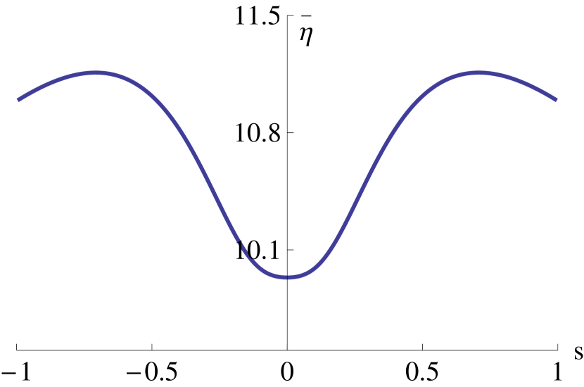
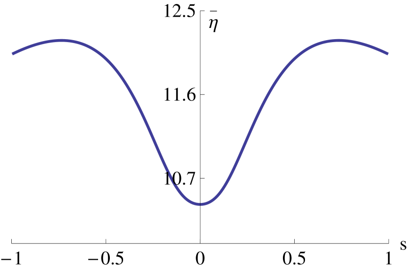
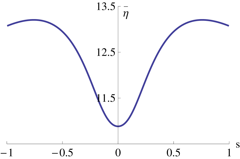
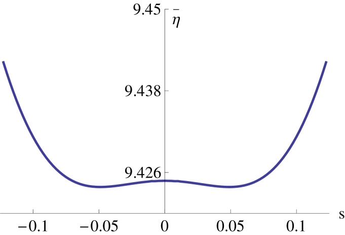
That is, there exists a curve { ( u ~ ( s ) , η ( s ) ) : | s | < δ } ⊂ U η 0 conditional-set ~ 𝑢 𝑠 𝜂 𝑠 𝑠 𝛿 subscript 𝑈 subscript 𝜂 0 \left\{\left(\tilde{u}(s),\eta(s)\right):|s|<\delta\right\}\subset U_{\eta_{0}} δ > 0 𝛿 0 \delta>0 ( u ~ ( 0 ) , η ( 0 ) ) = ( 0 , η 0 ) ~ 𝑢 0 𝜂 0 0 subscript 𝜂 0 \left(\tilde{u}(0),\eta(0)\right)=(0,\eta_{0}) u ~ ( s ) ≠ 0 ~ 𝑢 𝑠 0 \tilde{u}(s)\neq 0 s ≠ 0 𝑠 0 s\neq 0 G ¯ η 0 ( u ~ ( s ) , η ( s ) ) = 0 subscript ¯ 𝐺 subscript 𝜂 0 ~ 𝑢 𝑠 𝜂 𝑠 0 \bar{G}_{\eta_{0}}\left(\tilde{u}(s),\eta(s)\right)=0 | s | < δ 𝑠 𝛿 |s|<\delta G ¯ η 0 ( u ¯ , η ) = 0 subscript ¯ 𝐺 subscript 𝜂 0 ¯ 𝑢 𝜂 0 \bar{G}_{\eta_{0}}\left(\bar{u},\eta\right)=0 ( 0 , η 0 ) 0 subscript 𝜂 0 (0,\eta_{0})
Proof.
We calculate the linearisation of G ¯ η 0 ( u ¯ , η ) = P 0 [ G ( ψ η 0 ( u ¯ , η ) ) ] subscript ¯ 𝐺 subscript 𝜂 0 ¯ 𝑢 𝜂 subscript 𝑃 0 delimited-[] 𝐺 subscript 𝜓 subscript 𝜂 0 ¯ 𝑢 𝜂 \bar{G}_{\eta_{0}}(\bar{u},\eta)=P_{0}\left[G\left(\psi_{\eta_{0}}(\bar{u},\eta)\right)\right] u ¯ ¯ 𝑢 \bar{u} v ¯ ∈ h e , 0 2 , α ( [ 0 , d ] ) ¯ 𝑣 superscript subscript ℎ 𝑒 0
2 𝛼
0 𝑑 \bar{v}\in h_{e,0}^{2,\alpha}\left([0,d]\right)
(14) D 1 G ¯ η 0 ( u ¯ , η ) [ v ¯ ] = P 0 [ D G ( ψ η 0 ( u ¯ , η ) ) [ D 1 ψ η 0 ( u ¯ , η ) [ v ¯ ] ] ] . subscript 𝐷 1 subscript ¯ 𝐺 subscript 𝜂 0 ¯ 𝑢 𝜂 delimited-[] ¯ 𝑣 subscript 𝑃 0 delimited-[] 𝐷 𝐺 subscript 𝜓 subscript 𝜂 0 ¯ 𝑢 𝜂 delimited-[] subscript 𝐷 1 subscript 𝜓 subscript 𝜂 0 ¯ 𝑢 𝜂 delimited-[] ¯ 𝑣 D_{1}\bar{G}_{\eta_{0}}(\bar{u},\eta)[\bar{v}]=P_{0}\left[DG\left(\psi_{\eta_{0}}(\bar{u},\eta)\right)\left[D_{1}\psi_{\eta_{0}}(\bar{u},\eta)[\bar{v}]\right]\right].
To simplify the calculation of D G ( u ) 𝐷 𝐺 𝑢 DG(u) W ( u ) = F ( 𝜿 u ) Ξ ( 𝜿 u ) u n − 1 L ( u ) ∫ 𝒮 d π 1 Ξ ( 𝜿 u ) u n − 1 L ( u ) 𝑑 z 𝑊 𝑢 𝐹 subscript 𝜿 𝑢 Ξ subscript 𝜿 𝑢 superscript 𝑢 𝑛 1 𝐿 𝑢 subscript superscript subscript 𝒮 𝑑 𝜋 1 Ξ subscript 𝜿 𝑢 superscript 𝑢 𝑛 1 𝐿 𝑢 differential-d 𝑧 W(u)=\frac{F\left(\bm{\kappa}_{u}\right)\Xi\left(\bm{\kappa}_{u}\right)u^{n-1}L(u)}{\int_{\mathscr{S}_{\frac{d}{\pi}}^{1}}\Xi\left(\bm{\kappa}_{u}\right)u^{n-1}L(u)\,dz} D L ( u ) [ v ] = u ′ v ′ L ( u ) 𝐷 𝐿 𝑢 delimited-[] 𝑣 superscript 𝑢 ′ superscript 𝑣 ′ 𝐿 𝑢 DL(u)[v]=\frac{u^{\prime}v^{\prime}}{L(u)}
D G ( u ) [ v ] = 𝐷 𝐺 𝑢 delimited-[] 𝑣 absent \displaystyle DG(u)[v]= u ′ v ′ L ( u ) ( ∫ 𝒮 d π 1 W ( u ) 𝑑 z − F ( 𝜿 u ) ) + L ( u ) ( ∫ 𝒮 d π 1 D W ( u ) [ v ] 𝑑 z − D ( F ( 𝜿 u ) ) [ v ] ) superscript 𝑢 ′ superscript 𝑣 ′ 𝐿 𝑢 subscript superscript subscript 𝒮 𝑑 𝜋 1 𝑊 𝑢 differential-d 𝑧 𝐹 subscript 𝜿 𝑢 𝐿 𝑢 subscript superscript subscript 𝒮 𝑑 𝜋 1 𝐷 𝑊 𝑢 delimited-[] 𝑣 differential-d 𝑧 𝐷 𝐹 subscript 𝜿 𝑢 delimited-[] 𝑣 \displaystyle\frac{u^{\prime}v^{\prime}}{L(u)}\left(\int_{\mathscr{S}_{\frac{d}{\pi}}^{1}}W(u)\,dz-F\left(\bm{\kappa}_{u}\right)\right)+L(u)\left(\int_{\mathscr{S}_{\frac{d}{\pi}}^{1}}DW(u)[v]\,dz-D\left(F\left(\bm{\kappa}_{u}\right)\right)[v]\right)
(15) = \displaystyle= u ′ v ′ G ( u ) L ( u ) 2 + L ( u ) ( ∫ 𝒮 d π 1 D W ( u ) [ v ] 𝑑 z − D ( F ( 𝜿 u ) ) [ v ] ) . superscript 𝑢 ′ superscript 𝑣 ′ 𝐺 𝑢 𝐿 superscript 𝑢 2 𝐿 𝑢 subscript superscript subscript 𝒮 𝑑 𝜋 1 𝐷 𝑊 𝑢 delimited-[] 𝑣 differential-d 𝑧 𝐷 𝐹 subscript 𝜿 𝑢 delimited-[] 𝑣 \displaystyle\frac{u^{\prime}v^{\prime}G(u)}{L(u)^{2}}+L(u)\left(\int_{\mathscr{S}_{\frac{d}{\pi}}^{1}}DW(u)[v]\,dz-D\left(F\left(\bm{\kappa}_{u}\right)\right)[v]\right).
If we linearise W 𝑊 W u = n − 1 η 𝑢 𝑛 1 𝜂 u=\frac{n-1}{\eta}
∫ 𝒮 d π 1 D W ( n − 1 η ) [ v ] 𝑑 z = ⨏ 𝒮 d π 1 D ( F ( 𝜿 u ) ) | u = n − 1 η [ v ] d z . subscript superscript subscript 𝒮 𝑑 𝜋 1 𝐷 𝑊 𝑛 1 𝜂 delimited-[] 𝑣 differential-d 𝑧 evaluated-at subscript superscript subscript 𝒮 𝑑 𝜋 1 𝐷 𝐹 subscript 𝜿 𝑢 𝑢 𝑛 1 𝜂 delimited-[] 𝑣 𝑑 𝑧 \int_{\mathscr{S}_{\frac{d}{\pi}}^{1}}DW\left(\frac{n-1}{\eta}\right)[v]\,dz=\fint_{\mathscr{S}_{\frac{d}{\pi}}^{1}}\left.D\left(F\left(\bm{\kappa}_{u}\right)\right)\right|_{u=\frac{n-1}{\eta}}[v]\,dz.
Substituting this into (3
(16) D G ( n − 1 η ) [ v ] = ⨏ 𝒮 d π 1 D ( F ( 𝜿 u ) ) | u = n − 1 η [ v ] d z − D ( F ( 𝜿 u ) ) | u = n − 1 η [ v ] , 𝐷 𝐺 𝑛 1 𝜂 delimited-[] 𝑣 evaluated-at subscript superscript subscript 𝒮 𝑑 𝜋 1 𝐷 𝐹 subscript 𝜿 𝑢 𝑢 𝑛 1 𝜂 delimited-[] 𝑣 𝑑 𝑧 evaluated-at 𝐷 𝐹 subscript 𝜿 𝑢 𝑢 𝑛 1 𝜂 delimited-[] 𝑣 DG\left(\frac{n-1}{\eta}\right)[v]=\fint_{\mathscr{S}_{\frac{d}{\pi}}^{1}}\left.D\left(F\left(\bm{\kappa}_{u}\right)\right)\right|_{u=\frac{n-1}{\eta}}[v]\,dz-\left.D\left(F\left(\bm{\kappa}_{u}\right)\right)\right|_{u=\frac{n-1}{\eta}}[v],
Therefore using (11 14 G ¯ η 0 subscript ¯ 𝐺 subscript 𝜂 0 \bar{G}_{\eta_{0}} ( 0 , η ) 0 𝜂 (0,\eta)
(17) D 1 G ¯ η 0 ( 0 , η ) [ v ¯ ] = subscript 𝐷 1 subscript ¯ 𝐺 subscript 𝜂 0 0 𝜂 delimited-[] ¯ 𝑣 absent \displaystyle D_{1}\bar{G}_{\eta_{0}}(0,\eta)[\bar{v}]= D G ( n − 1 η ) [ v ¯ ] 𝐷 𝐺 𝑛 1 𝜂 delimited-[] ¯ 𝑣 \displaystyle DG\left(\frac{n-1}{\eta}\right)[\bar{v}]
= \displaystyle= ⨏ 𝒮 d π 1 D ( F ( 𝜿 u ) ) | u = n − 1 η [ v ¯ ] d z − D ( F ( 𝜿 u ) ) | u = n − 1 η [ v ¯ ] . evaluated-at subscript superscript subscript 𝒮 𝑑 𝜋 1 𝐷 𝐹 subscript 𝜿 𝑢 𝑢 𝑛 1 𝜂 delimited-[] ¯ 𝑣 𝑑 𝑧 evaluated-at 𝐷 𝐹 subscript 𝜿 𝑢 𝑢 𝑛 1 𝜂 delimited-[] ¯ 𝑣 \displaystyle\fint_{\mathscr{S}_{\frac{d}{\pi}}^{1}}\left.D\left(F\left(\bm{\kappa}_{u}\right)\right)\right|_{u=\frac{n-1}{\eta}}[\bar{v}]\,dz-\left.D\left(F\left(\bm{\kappa}_{u}\right)\right)\right|_{u=\frac{n-1}{\eta}}[\bar{v}].
To calculate the linearisation of F ( 𝜿 u ) 𝐹 subscript 𝜿 𝑢 F\left(\bm{\kappa}_{u}\right)
(18) D ( F ( 𝜿 u ) ) [ v ] = ( n − 1 ) ∂ F ∂ κ 1 ( 𝜿 u ) D κ 1 ( u ) [ v ] + ∂ F ∂ κ n ( 𝜿 u ) D κ n ( u ) [ v ] , 𝐷 𝐹 subscript 𝜿 𝑢 delimited-[] 𝑣 𝑛 1 𝐹 subscript 𝜅 1 subscript 𝜿 𝑢 𝐷 subscript 𝜅 1 𝑢 delimited-[] 𝑣 𝐹 subscript 𝜅 𝑛 subscript 𝜿 𝑢 𝐷 subscript 𝜅 𝑛 𝑢 delimited-[] 𝑣 D\left(F\left(\bm{\kappa}_{u}\right)\right)[v]=(n-1)\frac{\partial F}{\partial\kappa_{1}}\left(\bm{\kappa}_{u}\right)D\kappa_{1}(u)[v]+\frac{\partial F}{\partial\kappa_{n}}\left(\bm{\kappa}_{u}\right)D\kappa_{n}(u)[v],
where
κ 1 ( u ) = 1 u L ( u ) , κ n ( u ) = − u ′′ L ( u ) 3 . formulae-sequence subscript 𝜅 1 𝑢 1 𝑢 𝐿 𝑢 subscript 𝜅 𝑛 𝑢 superscript 𝑢 ′′ 𝐿 superscript 𝑢 3 \kappa_{1}(u)=\frac{1}{uL(u)},\ \ \ \kappa_{n}(u)=-\frac{u^{\prime\prime}}{L(u)^{3}}.
Taking the linearisation of the curvatures:
(19) D κ 1 ( u ) [ v ] = − v u 2 L ( u ) − u ′ v ′ u L ( u ) 3 , D κ n ( u ) [ v ] = − v ′′ L ( u ) 3 + 3 u ′′ u ′ v ′ L ( u ) 5 , formulae-sequence 𝐷 subscript 𝜅 1 𝑢 delimited-[] 𝑣 𝑣 superscript 𝑢 2 𝐿 𝑢 superscript 𝑢 ′ superscript 𝑣 ′ 𝑢 𝐿 superscript 𝑢 3 𝐷 subscript 𝜅 𝑛 𝑢 delimited-[] 𝑣 superscript 𝑣 ′′ 𝐿 superscript 𝑢 3 3 superscript 𝑢 ′′ superscript 𝑢 ′ superscript 𝑣 ′ 𝐿 superscript 𝑢 5 D\kappa_{1}(u)[v]=\frac{-v}{u^{2}L(u)}-\frac{u^{\prime}v^{\prime}}{uL(u)^{3}},\ \ \ D\kappa_{n}(u)[v]=-\frac{v^{\prime\prime}}{L(u)^{3}}+\frac{3u^{\prime\prime}u^{\prime}v^{\prime}}{L(u)^{5}},
therefore
(20) D κ 1 ( n − 1 η ) [ v ] = − ( η n − 1 ) 2 v , D κ n ( n − 1 η ) [ v ] = − v ′′ . formulae-sequence 𝐷 subscript 𝜅 1 𝑛 1 𝜂 delimited-[] 𝑣 superscript 𝜂 𝑛 1 2 𝑣 𝐷 subscript 𝜅 𝑛 𝑛 1 𝜂 delimited-[] 𝑣 superscript 𝑣 ′′ D\kappa_{1}\left(\frac{n-1}{\eta}\right)[v]=-\left(\frac{\eta}{n-1}\right)^{2}v,\ \ \ D\kappa_{n}\left(\frac{n-1}{\eta}\right)[v]=-v^{\prime\prime}.
Substituting this into (18
(21) D ( F ( 𝜿 u ) ) | u = n − 1 η [ v ] = − ( F n ( η ) v ′′ + η 2 F 1 ( η ) n − 1 v ) . evaluated-at 𝐷 𝐹 subscript 𝜿 𝑢 𝑢 𝑛 1 𝜂 delimited-[] 𝑣 subscript 𝐹 𝑛 𝜂 superscript 𝑣 ′′ superscript 𝜂 2 subscript 𝐹 1 𝜂 𝑛 1 𝑣 \left.D\left(F\left(\bm{\kappa}_{u}\right)\right)\right|_{u=\frac{n-1}{\eta}}[v]=-\left(F_{n}(\eta)v^{\prime\prime}+\frac{\eta^{2}F_{1}(\eta)}{n-1}v\right).
By (17
(22) D 1 G ¯ η 0 ( 0 , η ) [ v ¯ ] = F n ( η ) v ¯ ′′ + η 2 F 1 ( η ) ( n − 1 ) v ¯ . subscript 𝐷 1 subscript ¯ 𝐺 subscript 𝜂 0 0 𝜂 delimited-[] ¯ 𝑣 subscript 𝐹 𝑛 𝜂 superscript ¯ 𝑣 ′′ superscript 𝜂 2 subscript 𝐹 1 𝜂 𝑛 1 ¯ 𝑣 D_{1}\bar{G}_{\eta_{0}}(0,\eta)[\bar{v}]=F_{n}(\eta)\bar{v}^{\prime\prime}+\frac{\eta^{2}F_{1}(\eta)}{(n-1)}\bar{v}.
This map is a bijection from h e , 0 2 , α ( 𝒮 d π 1 ) superscript subscript ℎ 𝑒 0
2 𝛼
superscript subscript 𝒮 𝑑 𝜋 1 h_{e,0}^{2,\alpha}\left(\mathscr{S}_{\frac{d}{\pi}}^{1}\right) h e , 0 0 , α ( 𝒮 d π 1 ) superscript subscript ℎ 𝑒 0
0 𝛼
superscript subscript 𝒮 𝑑 𝜋 1 h_{e,0}^{0,\alpha}\left(\mathscr{S}_{\frac{d}{\pi}}^{1}\right) η = m π d ( n − 1 ) F n ( η ) F 1 ( η ) 𝜂 𝑚 𝜋 𝑑 𝑛 1 subscript 𝐹 𝑛 𝜂 subscript 𝐹 1 𝜂 \eta=\frac{m\pi}{d}\sqrt{\frac{(n-1)F_{n}(\eta)}{F_{1}(\eta)}} m ∈ ℕ 𝑚 ℕ m\in\mathbb{N} F 1 ( η ) = F n ( η ) = 0 subscript 𝐹 1 𝜂 subscript 𝐹 𝑛 𝜂 0 F_{1}(\eta)=F_{n}(\eta)=0 η = n − 1 R c r i t 𝜂 𝑛 1 subscript 𝑅 𝑐 𝑟 𝑖 𝑡 \eta=\frac{n-1}{R_{crit}}
When η = m π d ( n − 1 ) F n ( η ) F 1 ( η ) 𝜂 𝑚 𝜋 𝑑 𝑛 1 subscript 𝐹 𝑛 𝜂 subscript 𝐹 1 𝜂 \eta=\frac{m\pi}{d}\sqrt{\frac{(n-1)F_{n}(\eta)}{F_{1}(\eta)}}
N ( D 1 G ¯ η 0 ( 0 , η ) ) = 𝑁 subscript 𝐷 1 subscript ¯ 𝐺 subscript 𝜂 0 0 𝜂 absent \displaystyle N\left(D_{1}\bar{G}_{\eta_{0}}(0,\eta)\right)= span ( cos ( m π z d ) ) span 𝑚 𝜋 𝑧 𝑑 \displaystyle\text{span}\left(\cos\left(\frac{m\pi z}{d}\right)\right)
R ( D 1 G ¯ η 0 ( 0 , η ) ) = 𝑅 subscript 𝐷 1 subscript ¯ 𝐺 subscript 𝜂 0 0 𝜂 absent \displaystyle R\left(D_{1}\bar{G}_{\eta_{0}}(0,\eta)\right)= h e , 0 0 , α ( 𝒮 d π 1 ) / cos ( m π z d ) . superscript subscript ℎ 𝑒 0
0 𝛼
superscript subscript 𝒮 𝑑 𝜋 1 𝑚 𝜋 𝑧 𝑑 \displaystyle h_{e,0}^{0,\alpha}\left(\mathscr{S}_{\frac{d}{\pi}}^{1}\right)/\cos\left(\frac{m\pi z}{d}\right).
Also, from (22
D 12 2 G ¯ η 0 ( 0 , η ) [ v ¯ ] = superscript subscript 𝐷 12 2 subscript ¯ 𝐺 subscript 𝜂 0 0 𝜂 delimited-[] ¯ 𝑣 absent \displaystyle D_{12}^{2}\bar{G}_{\eta_{0}}\left(0,\eta\right)[\bar{v}]= F n ′ ( η ) v ¯ ′′ + ( 2 η F 1 ( η ) n − 1 + η 2 F 1 ′ ( η ) n − 1 ) v ¯ superscript subscript 𝐹 𝑛 ′ 𝜂 superscript ¯ 𝑣 ′′ 2 𝜂 subscript 𝐹 1 𝜂 𝑛 1 superscript 𝜂 2 superscript subscript 𝐹 1 ′ 𝜂 𝑛 1 ¯ 𝑣 \displaystyle F_{n}^{\prime}(\eta)\bar{v}^{\prime\prime}+\left(\frac{2\eta F_{1}(\eta)}{n-1}+\frac{\eta^{2}F_{1}^{\prime}(\eta)}{n-1}\right)\bar{v}
(23) = \displaystyle= F n ′ ( η ) F n ( η ) D 1 G ¯ η 0 ( 0 , η ) [ v ¯ ] + η n − 1 ( 2 F 1 ( η ) + η ( F 1 ′ ( η ) − F 1 ( η ) F n ′ ( η ) F n ( η ) ) ) v ¯ . superscript subscript 𝐹 𝑛 ′ 𝜂 subscript 𝐹 𝑛 𝜂 subscript 𝐷 1 subscript ¯ 𝐺 subscript 𝜂 0 0 𝜂 delimited-[] ¯ 𝑣 𝜂 𝑛 1 2 subscript 𝐹 1 𝜂 𝜂 superscript subscript 𝐹 1 ′ 𝜂 subscript 𝐹 1 𝜂 superscript subscript 𝐹 𝑛 ′ 𝜂 subscript 𝐹 𝑛 𝜂 ¯ 𝑣 \displaystyle\frac{F_{n}^{\prime}(\eta)}{F_{n}(\eta)}D_{1}\bar{G}_{\eta_{0}}(0,\eta)[\bar{v}]+\frac{\eta}{n-1}\left(2F_{1}(\eta)+\eta\left(F_{1}^{\prime}(\eta)-\frac{F_{1}(\eta)F_{n}^{\prime}(\eta)}{F_{n}(\eta)}\right)\right)\bar{v}.
Therefore when η 𝜂 \eta η = m π d ( n − 1 ) F n ( η ) F 1 ( η ) 𝜂 𝑚 𝜋 𝑑 𝑛 1 subscript 𝐹 𝑛 𝜂 subscript 𝐹 1 𝜂 \eta=\frac{m\pi}{d}\sqrt{\frac{(n-1)F_{n}(\eta)}{F_{1}(\eta)}}
D 12 2 G ¯ η 0 ( 0 , η ) [ cos ( m π z d ) ] = η n − 1 ( 2 F 1 ( η ) + η ( F 1 ′ ( η ) − F 1 ( η ) F n ′ ( η ) F n ( η ) ) ) cos ( m π z d ) . superscript subscript 𝐷 12 2 subscript ¯ 𝐺 subscript 𝜂 0 0 𝜂 delimited-[] 𝑚 𝜋 𝑧 𝑑 𝜂 𝑛 1 2 subscript 𝐹 1 𝜂 𝜂 superscript subscript 𝐹 1 ′ 𝜂 subscript 𝐹 1 𝜂 superscript subscript 𝐹 𝑛 ′ 𝜂 subscript 𝐹 𝑛 𝜂 𝑚 𝜋 𝑧 𝑑 D_{12}^{2}\bar{G}_{\eta_{0}}\left(0,\eta\right)\left[\cos\left(\frac{m\pi z}{d}\right)\right]=\frac{\eta}{n-1}\left(2F_{1}(\eta)+\eta\left(F_{1}^{\prime}(\eta)-\frac{F_{1}(\eta)F_{n}^{\prime}(\eta)}{F_{n}(\eta)}\right)\right)\cos\left(\frac{m\pi z}{d}\right).
To apply Theorem I.5.1 in [12 ] we require that D 12 2 G ¯ η 0 ( 0 , η ) [ cos ( m π z d ) ] ∉ R ( D 1 G ¯ η 0 ( 0 , η ) ) superscript subscript 𝐷 12 2 subscript ¯ 𝐺 subscript 𝜂 0 0 𝜂 delimited-[] 𝑚 𝜋 𝑧 𝑑 𝑅 subscript 𝐷 1 subscript ¯ 𝐺 subscript 𝜂 0 0 𝜂 D_{12}^{2}\bar{G}_{\eta_{0}}\left(0,\eta\right)\left[\cos\left(\frac{m\pi z}{d}\right)\right]\notin R\left(D_{1}\bar{G}_{\eta_{0}}(0,\eta)\right)
(24) 2 F 1 ( η ) + η ( F 1 ′ ( η ) − F 1 ( η ) F n ′ ( η ) F n ( η ) ) ≠ 0 . 2 subscript 𝐹 1 𝜂 𝜂 superscript subscript 𝐹 1 ′ 𝜂 subscript 𝐹 1 𝜂 superscript subscript 𝐹 𝑛 ′ 𝜂 subscript 𝐹 𝑛 𝜂 0 2F_{1}(\eta)+\eta\left(F_{1}^{\prime}(\eta)-\frac{F_{1}(\eta)F_{n}^{\prime}(\eta)}{F_{n}(\eta)}\right)\neq 0.
To prove this is the case when η = n − 1 R c r i t 𝜂 𝑛 1 subscript 𝑅 𝑐 𝑟 𝑖 𝑡 \eta=\frac{n-1}{R_{crit}} (A5) the function f ( η ) = η 2 n − 1 F 1 ( η ) − π 2 d 2 F n ( η ) 𝑓 𝜂 superscript 𝜂 2 𝑛 1 subscript 𝐹 1 𝜂 superscript 𝜋 2 superscript 𝑑 2 subscript 𝐹 𝑛 𝜂 f(\eta)=\frac{\eta^{2}}{n-1}F_{1}(\eta)-\frac{\pi^{2}}{d^{2}}F_{n}(\eta) η = n − 1 R c r i t 𝜂 𝑛 1 subscript 𝑅 𝑐 𝑟 𝑖 𝑡 \eta=\frac{n-1}{R_{crit}} f ′ ( n − 1 R c r i t ) ≠ 0 superscript 𝑓 ′ 𝑛 1 subscript 𝑅 𝑐 𝑟 𝑖 𝑡 0 f^{\prime}\left(\frac{n-1}{R_{crit}}\right)\neq 0
f ′ ( η ) = superscript 𝑓 ′ 𝜂 absent \displaystyle f^{\prime}(\eta)= 2 η n − 1 F 1 ( η ) + η 2 F 1 ′ ( η ) n − 1 − π 2 d 2 F n ′ ( η ) 2 𝜂 𝑛 1 subscript 𝐹 1 𝜂 superscript 𝜂 2 superscript subscript 𝐹 1 ′ 𝜂 𝑛 1 superscript 𝜋 2 superscript 𝑑 2 superscript subscript 𝐹 𝑛 ′ 𝜂 \displaystyle\frac{2\eta}{n-1}F_{1}(\eta)+\frac{\eta^{2}F_{1}^{\prime}(\eta)}{n-1}-\frac{\pi^{2}}{d^{2}}F_{n}^{\prime}(\eta)
= \displaystyle= η n − 1 ( 2 F 1 ( η ) + η ( F 1 ′ ( η ) − ( n − 1 ) 2 η 2 F 1 ( n − 1 R c r i t ) R c r i t 2 F n ( n − 1 R c r i t ) F n ′ ( η ) ) ) , 𝜂 𝑛 1 2 subscript 𝐹 1 𝜂 𝜂 superscript subscript 𝐹 1 ′ 𝜂 superscript 𝑛 1 2 superscript 𝜂 2 subscript 𝐹 1 𝑛 1 subscript 𝑅 𝑐 𝑟 𝑖 𝑡 superscript subscript 𝑅 𝑐 𝑟 𝑖 𝑡 2 subscript 𝐹 𝑛 𝑛 1 subscript 𝑅 𝑐 𝑟 𝑖 𝑡 superscript subscript 𝐹 𝑛 ′ 𝜂 \displaystyle\frac{\eta}{n-1}\left(2F_{1}(\eta)+\eta\left(F_{1}^{\prime}(\eta)-\frac{(n-1)^{2}\eta^{2}F_{1}\left(\frac{n-1}{R_{crit}}\right)}{R_{crit}^{2}F_{n}\left(\frac{n-1}{R_{crit}}\right)}F_{n}^{\prime}(\eta)\right)\right),
so that (24 η = n − 1 R c r i t 𝜂 𝑛 1 subscript 𝑅 𝑐 𝑟 𝑖 𝑡 \eta=\frac{n-1}{R_{crit}}
Corollary 3.2 .
There exists a continuously differentiable family of nontrivial, axially symmetric hypersurfaces that are stationary solutions to the flow (1 (A1) -(A5) for R ~ = R c r i t ~ 𝑅 subscript 𝑅 𝑐 𝑟 𝑖 𝑡 \tilde{R}=R_{crit} R c r i t subscript 𝑅 𝑐 𝑟 𝑖 𝑡 R_{crit} ρ ~ ( s ) := ψ η 0 ( u ~ ( s ) , η ( s ) ) | [ 0 , d ] assign ~ 𝜌 𝑠 evaluated-at subscript 𝜓 subscript 𝜂 0 ~ 𝑢 𝑠 𝜂 𝑠 0 𝑑 \tilde{\rho}(s):=\psi_{\eta_{0}}\left(\tilde{u}(s),\eta(s)\right)|_{[0,d]}
We now give a stronger corollary for when F 𝐹 F 1.4 1.2
Corollary 3.3 .
There exists a continuously differentiable family of nontrivial, axially symmetric hypersurfaces that are stationary solutions to the flow (1 (A1) -(A5)* satisfied at R ~ = n − 1 η m ~ 𝑅 𝑛 1 subscript 𝜂 𝑚 \tilde{R}=\frac{n-1}{\eta_{m}} η m := m π d ( n − 1 ) F n F 1 assign subscript 𝜂 𝑚 𝑚 𝜋 𝑑 𝑛 1 subscript 𝐹 𝑛 subscript 𝐹 1 \eta_{m}:=\frac{m\pi}{d}\sqrt{\frac{(n-1)F_{n}}{F_{1}}} n − 1 η m 𝑛 1 subscript 𝜂 𝑚 \frac{n-1}{\eta_{m}} ρ ~ m ( s ) := ψ η m ( u ~ m ( s ) , η m ( s ) ) | [ 0 , d ] assign subscript ~ 𝜌 𝑚 𝑠 evaluated-at subscript 𝜓 subscript 𝜂 𝑚 subscript ~ 𝑢 𝑚 𝑠 subscript 𝜂 𝑚 𝑠 0 𝑑 \tilde{\rho}_{m}(s):=\psi_{\eta_{m}}\left(\tilde{u}_{m}(s),\eta_{m}(s)\right)|_{[0,d]}
Proof.
Since F 𝐹 F (A2) reduces to F a ≠ 0 subscript 𝐹 𝑎 0 F_{a}\neq 0 a = 1 , n 𝑎 1 𝑛
a=1,n 22
(25) D 1 G ¯ η 0 ( 0 , η ) [ v ¯ ] = η k − 1 F n ( v ¯ ′′ + η 2 F 1 ( n − 1 ) F n v ¯ ) , subscript 𝐷 1 subscript ¯ 𝐺 subscript 𝜂 0 0 𝜂 delimited-[] ¯ 𝑣 superscript 𝜂 𝑘 1 subscript 𝐹 𝑛 superscript ¯ 𝑣 ′′ superscript 𝜂 2 subscript 𝐹 1 𝑛 1 subscript 𝐹 𝑛 ¯ 𝑣 D_{1}\bar{G}_{\eta_{0}}(0,\eta)[\bar{v}]=\eta^{k-1}F_{n}\left(\bar{v}^{\prime\prime}+\frac{\eta^{2}F_{1}}{(n-1)F_{n}}\bar{v}\right),
which is a bijection if and only if η ≠ η m 𝜂 subscript 𝜂 𝑚 \eta\neq\eta_{m} ( 0 , η m ) 0 subscript 𝜂 𝑚 (0,\eta_{m}) F a ′ ( η ) = ( k − 1 ) η k − 2 F a superscript subscript 𝐹 𝑎 ′ 𝜂 𝑘 1 superscript 𝜂 𝑘 2 subscript 𝐹 𝑎 F_{a}^{\prime}(\eta)=(k-1)\eta^{k-2}F_{a} a = 1 , n 𝑎 1 𝑛
a=1,n 24 F 1 ≠ 0 subscript 𝐹 1 0 F_{1}\neq 0 ( u ~ m ( s ) , η m ( s ) ) subscript ~ 𝑢 𝑚 𝑠 subscript 𝜂 𝑚 𝑠 (\tilde{u}_{m}(s),\eta_{m}(s))
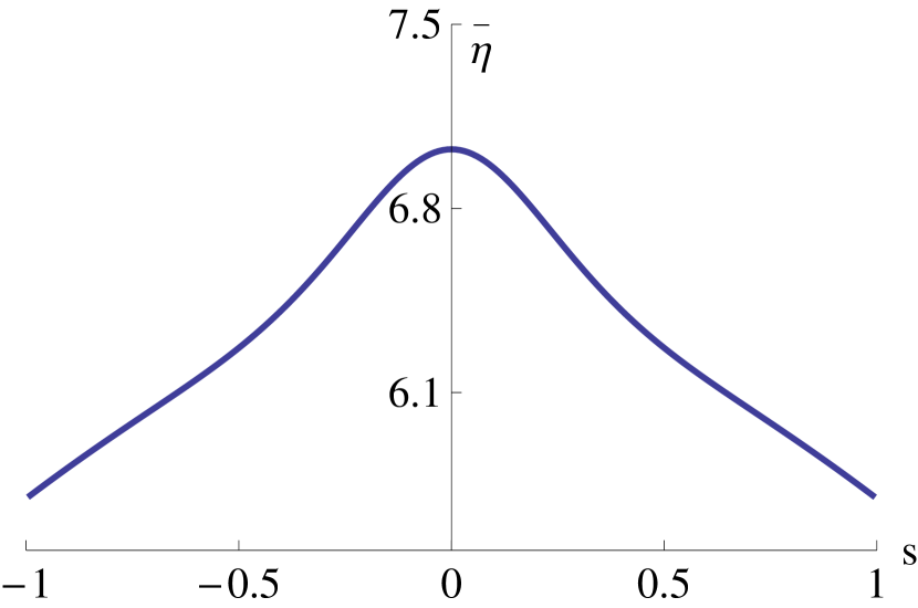
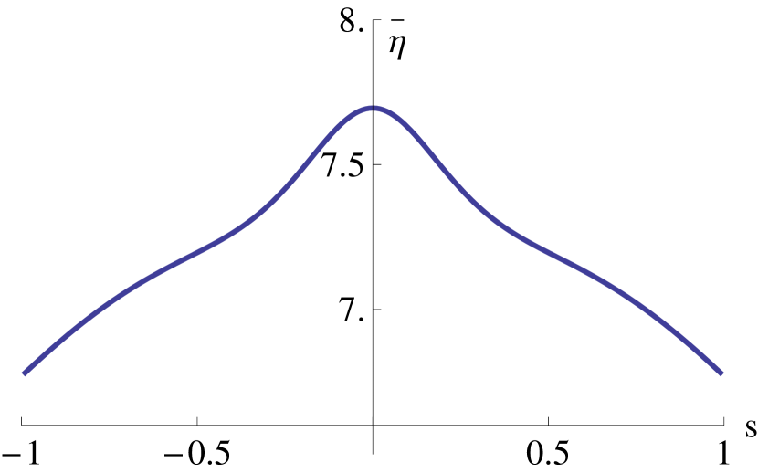
We will now consider the spectrum of D 1 G ¯ η 0 ( 0 , η ) subscript 𝐷 1 subscript ¯ 𝐺 subscript 𝜂 0 0 𝜂 D_{1}\bar{G}_{\eta_{0}}(0,\eta) 22 η < η 0 𝜂 subscript 𝜂 0 \eta<\eta_{0} η > η 0 𝜂 subscript 𝜂 0 \eta>\eta_{0} (A5) ) then the spectrum of D 1 G ¯ η 0 ( 0 , η ) subscript 𝐷 1 subscript ¯ 𝐺 subscript 𝜂 0 0 𝜂 D_{1}\bar{G}_{\eta_{0}}(0,\eta) 1.1 η = η 0 𝜂 subscript 𝜂 0 \eta=\eta_{0} ( 0 , η 0 ) 0 subscript 𝜂 0 \left(0,\eta_{0}\right)
To analyse the curve we make the following definitions:
v ^ := A cos ( η 0 F 1 ( η 0 ) ( n − 1 ) F n ( η 0 ) z ) , A := ‖ cos ( η 0 F 1 ( η 0 ) ( n − 1 ) F n ( η 0 ) z ) ‖ h 2 , α − 1 , formulae-sequence assign ^ 𝑣 𝐴 subscript 𝜂 0 subscript 𝐹 1 subscript 𝜂 0 𝑛 1 subscript 𝐹 𝑛 subscript 𝜂 0 𝑧 assign 𝐴 subscript superscript norm subscript 𝜂 0 subscript 𝐹 1 subscript 𝜂 0 𝑛 1 subscript 𝐹 𝑛 subscript 𝜂 0 𝑧 1 superscript ℎ 2 𝛼
\hat{v}:=A\cos\left(\eta_{0}\sqrt{\frac{F_{1}(\eta_{0})}{(n-1)F_{n}(\eta_{0})}}z\right),\ \ A:=\left\|\cos\left(\eta_{0}\sqrt{\frac{F_{1}(\eta_{0})}{(n-1)F_{n}(\eta_{0})}}z\right)\right\|^{-1}_{h^{2,\alpha}},
v ~ := B cos ( η 0 F 1 ( η 0 ) ( n − 1 ) F n ( η 0 ) z ) , B := ‖ cos ( η 0 F 1 ( η 0 ) ( n − 1 ) F n ( η 0 ) z ) ‖ h 0 , α − 1 , formulae-sequence assign ~ 𝑣 𝐵 subscript 𝜂 0 subscript 𝐹 1 subscript 𝜂 0 𝑛 1 subscript 𝐹 𝑛 subscript 𝜂 0 𝑧 assign 𝐵 subscript superscript norm subscript 𝜂 0 subscript 𝐹 1 subscript 𝜂 0 𝑛 1 subscript 𝐹 𝑛 subscript 𝜂 0 𝑧 1 superscript ℎ 0 𝛼
\tilde{v}:=B\cos\left(\eta_{0}\sqrt{\frac{F_{1}(\eta_{0})}{(n-1)F_{n}(\eta_{0})}}z\right),\ \ B:=\left\|\cos\left(\eta_{0}\sqrt{\frac{F_{1}(\eta_{0})}{(n-1)F_{n}(\eta_{0})}}z\right)\right\|^{-1}_{h^{0,\alpha}},
and
(26) v ~ ∗ [ v ¯ ] := 2 B ⨏ 𝒮 d π 1 v ¯ cos ( η 0 F 1 ( η 0 ) ( n − 1 ) F n ( η 0 ) z ) 𝑑 z , assign superscript ~ 𝑣 delimited-[] ¯ 𝑣 2 𝐵 subscript superscript subscript 𝒮 𝑑 𝜋 1 ¯ 𝑣 subscript 𝜂 0 subscript 𝐹 1 subscript 𝜂 0 𝑛 1 subscript 𝐹 𝑛 subscript 𝜂 0 𝑧 differential-d 𝑧 \tilde{v}^{*}[\bar{v}]:=\frac{2}{B}\fint_{\mathscr{S}_{\frac{d}{\pi}}^{1}}\bar{v}\cos\left(\eta_{0}\sqrt{\frac{F_{1}(\eta_{0})}{(n-1)F_{n}(\eta_{0})}}z\right)\,dz,
so that v ~ ∗ [ v ~ ] = 1 superscript ~ 𝑣 delimited-[] ~ 𝑣 1 \tilde{v}^{*}[\tilde{v}]=1 D 1 G ¯ η 0 ( 0 , η 0 ) subscript 𝐷 1 subscript ¯ 𝐺 subscript 𝜂 0 0 subscript 𝜂 0 D_{1}\bar{G}_{\eta_{0}}(0,\eta_{0}) L 2 superscript 𝐿 2 L^{2} v ~ ∗ [ D 1 G ¯ η 0 ( 0 , η 0 ) [ v ] ] = 0 superscript ~ 𝑣 delimited-[] subscript 𝐷 1 subscript ¯ 𝐺 subscript 𝜂 0 0 subscript 𝜂 0 delimited-[] 𝑣 0 \tilde{v}^{*}\left[D_{1}\bar{G}_{\eta_{0}}\left(0,\eta_{0}\right)[v]\right]=0 v ∈ h e 2 , α ( 𝒮 d π 1 ) 𝑣 superscript subscript ℎ 𝑒 2 𝛼
superscript subscript 𝒮 𝑑 𝜋 1 v\in h_{e}^{2,\alpha}\left(\mathscr{S}_{\frac{d}{\pi}}^{1}\right) η 0 subscript 𝜂 0 \eta_{0}
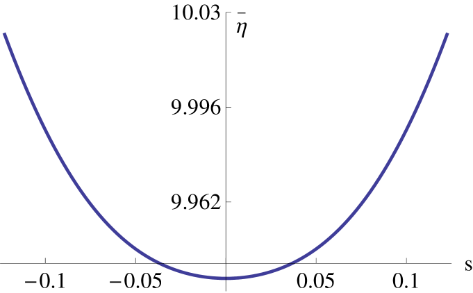
Theorem 3.4 .
Let (A1) -(A5) hold with R ~ = R c r i t ~ 𝑅 subscript 𝑅 𝑐 𝑟 𝑖 𝑡 \tilde{R}=R_{crit} 3.1
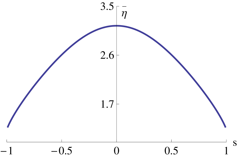
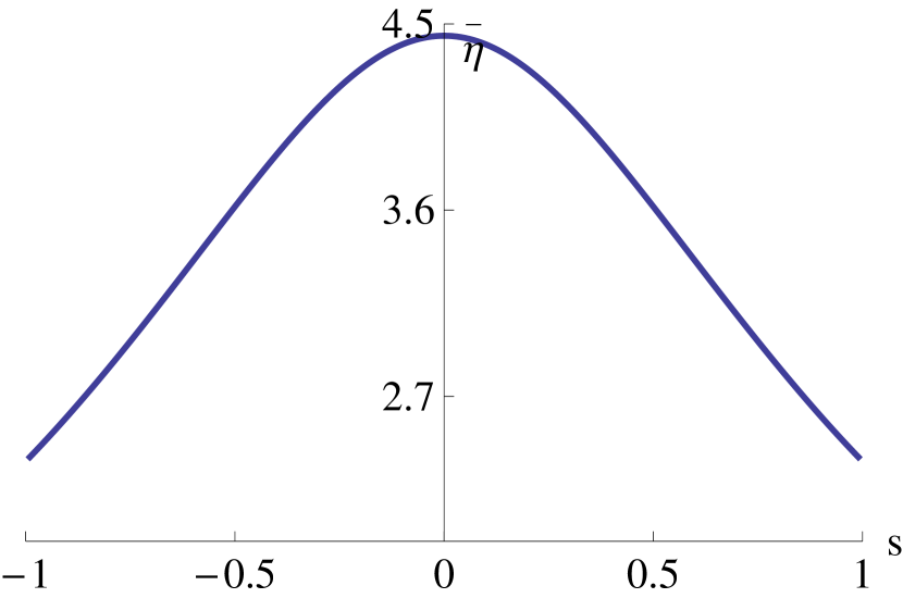
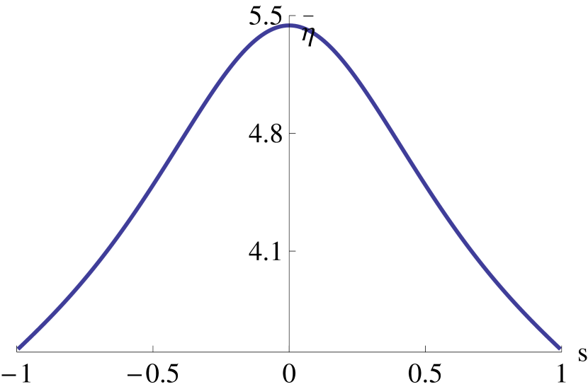
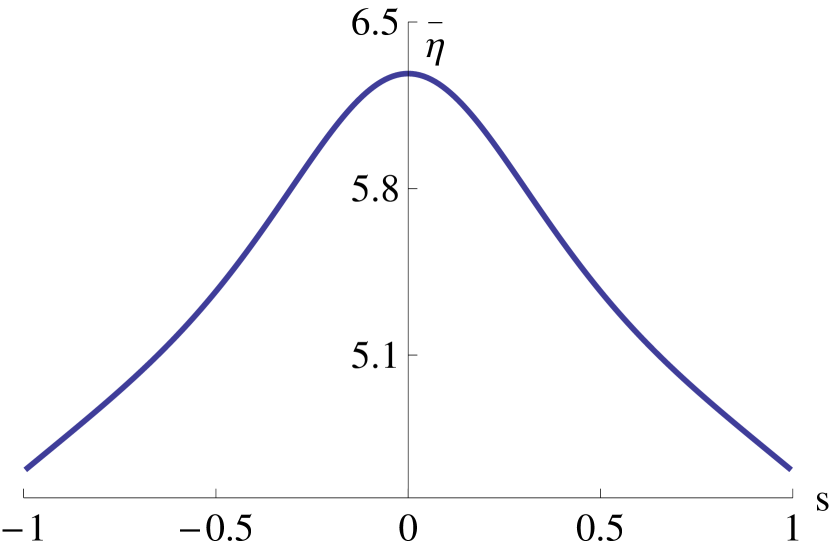
(27) η ′ ( 0 ) = 0 superscript 𝜂 ′ 0 0 \eta^{\prime}(0)=0
and
(28) η ′′ ( 0 ) = − η 0 3 A 2 12 ( ℱ 2 F 1 ( η 0 ) + η 0 F 1 ′ ( η 0 ) − η 0 F 1 ( η 0 ) F n ′ ( η 0 ) F n ( η 0 ) − 6 ∑ a = 1 n c a η 0 a ( n − 1 ) a ( ( n − 2 a − 1 ) − F 1 ( η 0 ) F n ( η 0 ) ( n − 1 a − 1 ) ) ( n − 1 ) ∑ a = 0 n c a η 0 a ( n − 1 ) a ( n − 1 a ) ) , superscript 𝜂 ′′ 0 superscript subscript 𝜂 0 3 superscript 𝐴 2 12 ℱ 2 subscript 𝐹 1 subscript 𝜂 0 subscript 𝜂 0 superscript subscript 𝐹 1 ′ subscript 𝜂 0 subscript 𝜂 0 subscript 𝐹 1 subscript 𝜂 0 superscript subscript 𝐹 𝑛 ′ subscript 𝜂 0 subscript 𝐹 𝑛 subscript 𝜂 0 6 superscript subscript 𝑎 1 𝑛 subscript 𝑐 𝑎 superscript subscript 𝜂 0 𝑎 superscript 𝑛 1 𝑎 binomial 𝑛 2 𝑎 1 subscript 𝐹 1 subscript 𝜂 0 subscript 𝐹 𝑛 subscript 𝜂 0 binomial 𝑛 1 𝑎 1 𝑛 1 superscript subscript 𝑎 0 𝑛 subscript 𝑐 𝑎 superscript subscript 𝜂 0 𝑎 superscript 𝑛 1 𝑎 binomial 𝑛 1 𝑎 \eta^{\prime\prime}(0)=\frac{-\eta_{0}^{3}A^{2}}{12}\left(\frac{\mathscr{F}}{2F_{1}(\eta_{0})+\eta_{0}F_{1}^{\prime}(\eta_{0})-\frac{\eta_{0}F_{1}(\eta_{0})F_{n}^{\prime}(\eta_{0})}{F_{n}(\eta_{0})}}-\frac{6\sum_{a=1}^{n}\frac{c_{a}\eta_{0}^{a}}{(n-1)^{a}}\left(\binom{n-2}{a-1}-\frac{F_{1}(\eta_{0})}{F_{n}(\eta_{0})}\binom{n-1}{a-1}\right)}{(n-1)\sum_{a=0}^{n}\frac{c_{a}\eta_{0}^{a}}{(n-1)^{a}}\binom{n-1}{a}}\right),
where
ℱ = ℱ absent \displaystyle\mathscr{F}= 3 η 0 2 F 1 ′′ ( η 0 ) ( n − 1 ) 2 − 9 η 0 2 F 1 ( η 0 ) F n ′′ ( η 0 ) ( n − 1 ) 2 F n ( η 0 ) + 9 η 0 2 F 1 ( η 0 ) 2 F n n ′ ( η 0 ) ( n − 1 ) 2 F n ( η 0 ) 2 − 3 η 0 2 F 1 ( η 0 ) 3 F n n n ( η 0 ) ( n − 1 ) 2 F n ( η 0 ) 3 3 superscript subscript 𝜂 0 2 superscript subscript 𝐹 1 ′′ subscript 𝜂 0 superscript 𝑛 1 2 9 superscript subscript 𝜂 0 2 subscript 𝐹 1 subscript 𝜂 0 superscript subscript 𝐹 𝑛 ′′ subscript 𝜂 0 superscript 𝑛 1 2 subscript 𝐹 𝑛 subscript 𝜂 0 9 superscript subscript 𝜂 0 2 subscript 𝐹 1 superscript subscript 𝜂 0 2 superscript subscript 𝐹 𝑛 𝑛 ′ subscript 𝜂 0 superscript 𝑛 1 2 subscript 𝐹 𝑛 superscript subscript 𝜂 0 2 3 superscript subscript 𝜂 0 2 subscript 𝐹 1 superscript subscript 𝜂 0 3 subscript 𝐹 𝑛 𝑛 𝑛 subscript 𝜂 0 superscript 𝑛 1 2 subscript 𝐹 𝑛 superscript subscript 𝜂 0 3 \displaystyle\frac{3\eta_{0}^{2}F_{1}^{\prime\prime}(\eta_{0})}{(n-1)^{2}}-\frac{9\eta_{0}^{2}F_{1}(\eta_{0})F_{n}^{\prime\prime}(\eta_{0})}{(n-1)^{2}F_{n}(\eta_{0})}+\frac{9\eta_{0}^{2}F_{1}(\eta_{0})^{2}F_{nn}^{\prime}(\eta_{0})}{(n-1)^{2}F_{n}(\eta_{0})^{2}}-\frac{3\eta_{0}^{2}F_{1}(\eta_{0})^{3}F_{nnn}(\eta_{0})}{(n-1)^{2}F_{n}(\eta_{0})^{3}}
+ η 0 2 F 1 ′ ( η 0 ) 2 ( n − 1 ) 2 F 1 ( η 0 ) − 7 η 0 2 F 1 ′ ( η 0 ) F n ′ ( η 0 ) ( n − 1 ) 2 F n ( η 0 ) + 5 η 0 2 F 1 ( η 0 ) F 1 ′ ( η 0 ) F n n ( η 0 ) ( n − 1 ) 2 F n ( η 0 ) 2 superscript subscript 𝜂 0 2 superscript subscript 𝐹 1 ′ superscript subscript 𝜂 0 2 superscript 𝑛 1 2 subscript 𝐹 1 subscript 𝜂 0 7 superscript subscript 𝜂 0 2 superscript subscript 𝐹 1 ′ subscript 𝜂 0 superscript subscript 𝐹 𝑛 ′ subscript 𝜂 0 superscript 𝑛 1 2 subscript 𝐹 𝑛 subscript 𝜂 0 5 superscript subscript 𝜂 0 2 subscript 𝐹 1 subscript 𝜂 0 superscript subscript 𝐹 1 ′ subscript 𝜂 0 subscript 𝐹 𝑛 𝑛 subscript 𝜂 0 superscript 𝑛 1 2 subscript 𝐹 𝑛 superscript subscript 𝜂 0 2 \displaystyle+\frac{\eta_{0}^{2}F_{1}^{\prime}(\eta_{0})^{2}}{(n-1)^{2}F_{1}(\eta_{0})}-\frac{7\eta_{0}^{2}F_{1}^{\prime}(\eta_{0})F_{n}^{\prime}(\eta_{0})}{(n-1)^{2}F_{n}(\eta_{0})}+\frac{5\eta_{0}^{2}F_{1}(\eta_{0})F_{1}^{\prime}(\eta_{0})F_{nn}(\eta_{0})}{(n-1)^{2}F_{n}(\eta_{0})^{2}}
+ 10 η 0 2 F 1 ( η 0 ) F n ′ ( η 0 ) 2 ( n − 1 ) 2 F n ( η 0 ) 2 − 13 η 0 2 F 1 ( η 0 ) 2 F n ′ ( η 0 ) F n n ( η 0 ) ( n − 1 ) 2 F n ( η 0 ) 3 + 4 η 0 2 F 1 ( η 0 ) 3 F n n ( η 0 ) 2 ( n − 1 ) 2 F n ( η 0 ) 4 10 superscript subscript 𝜂 0 2 subscript 𝐹 1 subscript 𝜂 0 superscript subscript 𝐹 𝑛 ′ superscript subscript 𝜂 0 2 superscript 𝑛 1 2 subscript 𝐹 𝑛 superscript subscript 𝜂 0 2 13 superscript subscript 𝜂 0 2 subscript 𝐹 1 superscript subscript 𝜂 0 2 superscript subscript 𝐹 𝑛 ′ subscript 𝜂 0 subscript 𝐹 𝑛 𝑛 subscript 𝜂 0 superscript 𝑛 1 2 subscript 𝐹 𝑛 superscript subscript 𝜂 0 3 4 superscript subscript 𝜂 0 2 subscript 𝐹 1 superscript subscript 𝜂 0 3 subscript 𝐹 𝑛 𝑛 superscript subscript 𝜂 0 2 superscript 𝑛 1 2 subscript 𝐹 𝑛 superscript subscript 𝜂 0 4 \displaystyle+\frac{10\eta_{0}^{2}F_{1}(\eta_{0})F_{n}^{\prime}(\eta_{0})^{2}}{(n-1)^{2}F_{n}(\eta_{0})^{2}}-\frac{13\eta_{0}^{2}F_{1}(\eta_{0})^{2}F_{n}^{\prime}(\eta_{0})F_{nn}(\eta_{0})}{(n-1)^{2}F_{n}(\eta_{0})^{3}}+\frac{4\eta_{0}^{2}F_{1}(\eta_{0})^{3}F_{nn}(\eta_{0})^{2}}{(n-1)^{2}F_{n}(\eta_{0})^{4}}
+ 2 ( 3 n + 8 ) η 0 F 1 ′ ( η 0 ) ( n − 1 ) 2 − 4 η 0 F 1 ( η 0 ) F 1 ′ ( η 0 ) ( n − 1 ) F n ( η 0 ) − 2 ( 3 n + 13 ) η 0 F 1 ( η 0 ) F n ′ ( η 0 ) ( n − 1 ) 2 F n ( η 0 ) 2 3 𝑛 8 subscript 𝜂 0 superscript subscript 𝐹 1 ′ subscript 𝜂 0 superscript 𝑛 1 2 4 subscript 𝜂 0 subscript 𝐹 1 subscript 𝜂 0 superscript subscript 𝐹 1 ′ subscript 𝜂 0 𝑛 1 subscript 𝐹 𝑛 subscript 𝜂 0 2 3 𝑛 13 subscript 𝜂 0 subscript 𝐹 1 subscript 𝜂 0 superscript subscript 𝐹 𝑛 ′ subscript 𝜂 0 superscript 𝑛 1 2 subscript 𝐹 𝑛 subscript 𝜂 0 \displaystyle+\frac{2(3n+8)\eta_{0}F_{1}^{\prime}(\eta_{0})}{(n-1)^{2}}-\frac{4\eta_{0}F_{1}(\eta_{0})F_{1}^{\prime}(\eta_{0})}{(n-1)F_{n}(\eta_{0})}-\frac{2(3n+13)\eta_{0}F_{1}(\eta_{0})F_{n}^{\prime}(\eta_{0})}{(n-1)^{2}F_{n}(\eta_{0})}
+ 2 η 0 F 1 ( η 0 ) 2 F n ′ ( η 0 ) ( n − 1 ) F n ( η 0 ) 2 + 10 η 0 F 1 ( η 0 ) 2 F n n ( η 0 ) ( n − 1 ) 2 F n ( η 0 ) 2 + 2 η 0 F 1 ( η 0 ) 3 F n n ( η 0 ) ( n − 1 ) F n ( η 0 ) 3 + 2 ( 6 n + 5 ) F 1 ( η 0 ) ( n − 1 ) 2 2 subscript 𝜂 0 subscript 𝐹 1 superscript subscript 𝜂 0 2 superscript subscript 𝐹 𝑛 ′ subscript 𝜂 0 𝑛 1 subscript 𝐹 𝑛 superscript subscript 𝜂 0 2 10 subscript 𝜂 0 subscript 𝐹 1 superscript subscript 𝜂 0 2 subscript 𝐹 𝑛 𝑛 subscript 𝜂 0 superscript 𝑛 1 2 subscript 𝐹 𝑛 superscript subscript 𝜂 0 2 2 subscript 𝜂 0 subscript 𝐹 1 superscript subscript 𝜂 0 3 subscript 𝐹 𝑛 𝑛 subscript 𝜂 0 𝑛 1 subscript 𝐹 𝑛 superscript subscript 𝜂 0 3 2 6 𝑛 5 subscript 𝐹 1 subscript 𝜂 0 superscript 𝑛 1 2 \displaystyle+\frac{2\eta_{0}F_{1}(\eta_{0})^{2}F_{n}^{\prime}(\eta_{0})}{(n-1)F_{n}(\eta_{0})^{2}}+\frac{10\eta_{0}F_{1}(\eta_{0})^{2}F_{nn}(\eta_{0})}{(n-1)^{2}F_{n}(\eta_{0})^{2}}+\frac{2\eta_{0}F_{1}(\eta_{0})^{3}F_{nn}(\eta_{0})}{(n-1)F_{n}(\eta_{0})^{3}}+\frac{2(6n+5)F_{1}(\eta_{0})}{(n-1)^{2}}
+ 4 F 1 ( η 0 ) 2 ( n − 1 ) F n ( η 0 ) − 2 F 1 ( η 0 ) 3 F n ( η 0 ) 2 , 4 subscript 𝐹 1 superscript subscript 𝜂 0 2 𝑛 1 subscript 𝐹 𝑛 subscript 𝜂 0 2 subscript 𝐹 1 superscript subscript 𝜂 0 3 subscript 𝐹 𝑛 superscript subscript 𝜂 0 2 \displaystyle+\frac{4F_{1}(\eta_{0})^{2}}{(n-1)F_{n}(\eta_{0})}-\frac{2F_{1}(\eta_{0})^{3}}{F_{n}(\eta_{0})^{2}},
and F a ( η ) = ∂ F ∂ κ a ( 𝛋 n − 1 η ) subscript 𝐹 𝑎 𝜂 𝐹 subscript 𝜅 𝑎 subscript 𝛋 𝑛 1 𝜂 F_{a}(\eta)=\frac{\partial F}{\partial\kappa_{a}}\left(\bm{\kappa}_{\frac{n-1}{\eta}}\right) F n n ( η ) = ∂ 2 F ∂ κ n 2 ( 𝛋 n − 1 η ) subscript 𝐹 𝑛 𝑛 𝜂 superscript 2 𝐹 superscript subscript 𝜅 𝑛 2 subscript 𝛋 𝑛 1 𝜂 F_{nn}(\eta)=\frac{\partial^{2}F}{\partial\kappa_{n}^{2}}\left(\bm{\kappa}_{\frac{n-1}{\eta}}\right) F n n n ( η ) = ∂ 3 F ∂ κ n 3 ( 𝛋 n − 1 η ) subscript 𝐹 𝑛 𝑛 𝑛 𝜂 superscript 3 𝐹 superscript subscript 𝜅 𝑛 3 subscript 𝛋 𝑛 1 𝜂 F_{nnn}(\eta)=\frac{\partial^{3}F}{\partial\kappa_{n}^{3}}\left(\bm{\kappa}_{\frac{n-1}{\eta}}\right)
Proof.
These formulas come from standard calculations using equations (I.6.3), (I.6.8) and (I.6.11) from [12 ] :
(29) η ′ ( 0 ) = − v ~ ∗ [ D 11 2 G ¯ ( 0 , η 0 ) [ v ^ , v ^ ] ] 2 v ~ ∗ [ D 12 2 G ¯ ( 0 , η 0 ) [ v ^ ] ] , superscript 𝜂 ′ 0 superscript ~ 𝑣 delimited-[] superscript subscript 𝐷 11 2 ¯ 𝐺 0 subscript 𝜂 0 ^ 𝑣 ^ 𝑣 2 superscript ~ 𝑣 delimited-[] superscript subscript 𝐷 12 2 ¯ 𝐺 0 subscript 𝜂 0 delimited-[] ^ 𝑣 \eta^{\prime}(0)=\frac{-\tilde{v}^{*}\left[D_{11}^{2}\bar{G}(0,\eta_{0})\left[\hat{v},\hat{v}\right]\right]}{2\tilde{v}^{*}\left[D_{12}^{2}\bar{G}(0,\eta_{0})\left[\hat{v}\right]\right]},
(30) η ′′ ( 0 ) = − v ~ ∗ [ D 111 3 G ¯ ( 0 , η 0 ) [ v ^ , v ^ , v ^ ] + 3 D 11 2 G ¯ ( 0 , η 0 ) [ v ^ , w ~ ] ] 3 v ~ ∗ [ D 12 2 G ¯ ( 0 , η 0 ) [ v ^ ] ] , superscript 𝜂 ′′ 0 superscript ~ 𝑣 delimited-[] superscript subscript 𝐷 111 3 ¯ 𝐺 0 subscript 𝜂 0 ^ 𝑣 ^ 𝑣 ^ 𝑣
3 superscript subscript 𝐷 11 2 ¯ 𝐺 0 subscript 𝜂 0 ^ 𝑣 ~ 𝑤 3 superscript ~ 𝑣 delimited-[] superscript subscript 𝐷 12 2 ¯ 𝐺 0 subscript 𝜂 0 delimited-[] ^ 𝑣 \eta^{\prime\prime}(0)=\frac{-\tilde{v}^{*}\left[D_{111}^{3}\bar{G}(0,\eta_{0})\left[\hat{v},\hat{v},\hat{v}\right]+3D_{11}^{2}\bar{G}(0,\eta_{0})\left[\hat{v},\tilde{w}\right]\right]}{3\tilde{v}^{*}\left[D_{12}^{2}\bar{G}(0,\eta_{0})\left[\hat{v}\right]\right]},
where w ~ ~ 𝑤 \tilde{w}
(31) D 1 G ¯ ( 0 , η 0 ) [ w ¯ ] = − D 11 2 G ¯ ( 0 , η 0 ) [ v ^ , v ^ ] , subscript 𝐷 1 ¯ 𝐺 0 subscript 𝜂 0 delimited-[] ¯ 𝑤 superscript subscript 𝐷 11 2 ¯ 𝐺 0 subscript 𝜂 0 ^ 𝑣 ^ 𝑣 D_{1}\bar{G}(0,\eta_{0})[\bar{w}]=-D_{11}^{2}\bar{G}(0,\eta_{0})\left[\hat{v},\hat{v}\right],
such that v ~ ∗ [ w ~ ] = 0 superscript ~ 𝑣 delimited-[] ~ 𝑤 0 \tilde{v}^{*}[\tilde{w}]=0 30 η ′ ( 0 ) = 0 superscript 𝜂 ′ 0 0 \eta^{\prime}(0)=0
By linearising (14
(32) D 11 2 G ¯ ( u ¯ , η ) [ v ¯ , w ¯ ] = superscript subscript 𝐷 11 2 ¯ 𝐺 ¯ 𝑢 𝜂 ¯ 𝑣 ¯ 𝑤 absent \displaystyle D_{11}^{2}\bar{G}(\bar{u},\eta)[\bar{v},\bar{w}]= P 0 [ D 2 G ( ψ ( u ¯ , η ) ) [ D 1 ψ ( u ¯ , η ) [ v ¯ ] , D 1 ψ ( u ¯ , η ) [ w ¯ ] ] ] subscript 𝑃 0 delimited-[] superscript 𝐷 2 𝐺 𝜓 ¯ 𝑢 𝜂 subscript 𝐷 1 𝜓 ¯ 𝑢 𝜂 delimited-[] ¯ 𝑣 subscript 𝐷 1 𝜓 ¯ 𝑢 𝜂 delimited-[] ¯ 𝑤 \displaystyle P_{0}\left[D^{2}G\left(\psi(\bar{u},\eta)\right)\left[D_{1}\psi(\bar{u},\eta)[\bar{v}],D_{1}\psi(\bar{u},\eta)[\bar{w}]\right]\right]
+ P 0 [ D G ( ψ ( u ¯ , η ) ) [ D 11 2 ψ ( u ¯ , η ) [ v ¯ , w ¯ ] ] ] , subscript 𝑃 0 delimited-[] 𝐷 𝐺 𝜓 ¯ 𝑢 𝜂 delimited-[] superscript subscript 𝐷 11 2 𝜓 ¯ 𝑢 𝜂 ¯ 𝑣 ¯ 𝑤 \displaystyle+P_{0}\left[DG\left(\psi(\bar{u},\eta)\right)\left[D_{11}^{2}\psi(\bar{u},\eta)[\bar{v},\bar{w}]\right]\right],
and from (11
(33) D 11 2 ψ ( 0 , η 0 ) [ v ¯ , w ¯ ] = superscript subscript 𝐷 11 2 𝜓 0 subscript 𝜂 0 ¯ 𝑣 ¯ 𝑤 absent \displaystyle D_{11}^{2}\psi(0,\eta_{0})[\bar{v},\bar{w}]= Ξ ( 𝜿 n − 1 η 0 ) − 1 ⨏ 𝒮 d π 1 v ¯ ( η 0 2 n − 1 ∂ Ξ ∂ κ 1 ( 𝜿 n − 1 η 0 ) w ¯ + ∂ Ξ ∂ κ n ( 𝜿 n − 1 η 0 ) w ¯ ′′ ) 𝑑 z Ξ superscript subscript 𝜿 𝑛 1 subscript 𝜂 0 1 subscript superscript subscript 𝒮 𝑑 𝜋 1 ¯ 𝑣 superscript subscript 𝜂 0 2 𝑛 1 Ξ subscript 𝜅 1 subscript 𝜿 𝑛 1 subscript 𝜂 0 ¯ 𝑤 Ξ subscript 𝜅 𝑛 subscript 𝜿 𝑛 1 subscript 𝜂 0 superscript ¯ 𝑤 ′′ differential-d 𝑧 \displaystyle\Xi\left(\bm{\kappa}_{\frac{n-1}{\eta_{0}}}\right)^{-1}\fint_{\mathscr{S}_{\frac{d}{\pi}}^{1}}\bar{v}\left(\frac{\eta_{0}^{2}}{n-1}\frac{\partial\Xi}{\partial\kappa_{1}}\left(\bm{\kappa}_{\frac{n-1}{\eta_{0}}}\right)\bar{w}+\frac{\partial\Xi}{\partial\kappa_{n}}\left(\bm{\kappa}_{\frac{n-1}{\eta_{0}}}\right)\bar{w}^{\prime\prime}\right)\,dz
− η 0 ⨏ 𝒮 d π 1 v ¯ w ¯ 𝑑 z . subscript 𝜂 0 subscript superscript subscript 𝒮 𝑑 𝜋 1 ¯ 𝑣 ¯ 𝑤 differential-d 𝑧 \displaystyle-\eta_{0}\fint_{\mathscr{S}_{\frac{d}{\pi}}^{1}}\bar{v}\bar{w}\,dz.
However at this stage it is only important that this is a constant function, so we associate it to its corresponding real number; in fact it is clear from (11 D 11 2 ψ ( u ¯ , η ) [ v ¯ , w ¯ ] superscript subscript 𝐷 11 2 𝜓 ¯ 𝑢 𝜂 ¯ 𝑣 ¯ 𝑤 D_{11}^{2}\psi(\bar{u},\eta)[\bar{v},\bar{w}] ( u ¯ , η ) ¯ 𝑢 𝜂 (\bar{u},\eta) 32
D 11 2 G ¯ ( 0 , η 0 ) = P 0 [ D 2 G ( n − 1 η 0 ) [ v ¯ , w ¯ ] + D 11 2 ψ ( 0 , η 0 ) [ v ¯ , w ¯ ] D G ( n − 1 η 0 ) [ 1 ] ] . superscript subscript 𝐷 11 2 ¯ 𝐺 0 subscript 𝜂 0 subscript 𝑃 0 delimited-[] superscript 𝐷 2 𝐺 𝑛 1 subscript 𝜂 0 ¯ 𝑣 ¯ 𝑤 superscript subscript 𝐷 11 2 𝜓 0 subscript 𝜂 0 ¯ 𝑣 ¯ 𝑤 𝐷 𝐺 𝑛 1 subscript 𝜂 0 delimited-[] 1 D_{11}^{2}\bar{G}(0,\eta_{0})=P_{0}\left[D^{2}G\left(\frac{n-1}{\eta_{0}}\right)[\bar{v},\bar{w}]+D_{11}^{2}\psi(0,\eta_{0})[\bar{v},\bar{w}]DG\left(\frac{n-1}{\eta_{0}}\right)[1]\right].
From (21 D ( F ( 𝜿 u ) ) | u = n − 1 η 0 [ 1 ] = − η 0 2 n − 1 F 1 ( η ) evaluated-at 𝐷 𝐹 subscript 𝜿 𝑢 𝑢 𝑛 1 subscript 𝜂 0 delimited-[] 1 superscript subscript 𝜂 0 2 𝑛 1 subscript 𝐹 1 𝜂 \left.D\left(F\left(\bm{\kappa}_{u}\right)\right)\right|_{u=\frac{n-1}{\eta_{0}}}[1]=-\frac{\eta_{0}^{2}}{n-1}F_{1}(\eta) 16 D G ( n − 1 η 0 ) [ 1 ] = 0 𝐷 𝐺 𝑛 1 subscript 𝜂 0 delimited-[] 1 0 DG\left(\frac{n-1}{\eta_{0}}\right)[1]=0
D 11 2 G ¯ ( 0 , η 0 ) = P 0 [ D 2 G ( n − 1 η 0 ) [ v ¯ , w ¯ ] ] . superscript subscript 𝐷 11 2 ¯ 𝐺 0 subscript 𝜂 0 subscript 𝑃 0 delimited-[] superscript 𝐷 2 𝐺 𝑛 1 subscript 𝜂 0 ¯ 𝑣 ¯ 𝑤 D_{11}^{2}\bar{G}(0,\eta_{0})=P_{0}\left[D^{2}G\left(\frac{n-1}{\eta_{0}}\right)[\bar{v},\bar{w}]\right].
Using (3
(34) D 2 G ( u ) [ v , w ] = superscript 𝐷 2 𝐺 𝑢 𝑣 𝑤 absent \displaystyle D^{2}G(u)[v,w]= w ′ v ′ G ( u ) + u ′ ( v ′ D G ( u ) [ w ] + w ′ D G ( u ) [ v ] ) L ( u ) 2 − 3 u ′ 2 v ′ w ′ G ( u ) L ( u ) 4 superscript 𝑤 ′ superscript 𝑣 ′ 𝐺 𝑢 superscript 𝑢 ′ superscript 𝑣 ′ 𝐷 𝐺 𝑢 delimited-[] 𝑤 superscript 𝑤 ′ 𝐷 𝐺 𝑢 delimited-[] 𝑣 𝐿 superscript 𝑢 2 3 superscript 𝑢 ′ 2
superscript 𝑣 ′ superscript 𝑤 ′ 𝐺 𝑢 𝐿 superscript 𝑢 4 \displaystyle\frac{w^{\prime}v^{\prime}G(u)+u^{\prime}\left(v^{\prime}DG(u)[w]+w^{\prime}DG(u)[v]\right)}{L(u)^{2}}-\frac{3u^{\prime 2}v^{\prime}w^{\prime}G(u)}{L(u)^{4}}
+ L ( u ) ( ∫ 𝒮 d π 1 D 2 W ( u ) [ v , w ] 𝑑 z − D 2 ( F ( 𝜿 u ) ) [ v , w ] ) , 𝐿 𝑢 subscript superscript subscript 𝒮 𝑑 𝜋 1 superscript 𝐷 2 𝑊 𝑢 𝑣 𝑤 differential-d 𝑧 superscript 𝐷 2 𝐹 subscript 𝜿 𝑢 𝑣 𝑤 \displaystyle+L(u)\left(\int_{\mathscr{S}_{\frac{d}{\pi}}^{1}}D^{2}W(u)[v,w]\,dz-D^{2}\left(F\left(\bm{\kappa}_{u}\right)\right)[v,w]\right),
which reduces to
D 2 G ( n − 1 η 0 ) [ v , w ] = ∫ 𝒮 d π 1 D 2 W ( n − 1 η 0 ) [ v , w ] 𝑑 z − D 2 ( F ( 𝜿 u ) ) | u = n − 1 η 0 [ v , w ] . superscript 𝐷 2 𝐺 𝑛 1 subscript 𝜂 0 𝑣 𝑤 subscript superscript subscript 𝒮 𝑑 𝜋 1 superscript 𝐷 2 𝑊 𝑛 1 subscript 𝜂 0 𝑣 𝑤 differential-d 𝑧 evaluated-at superscript 𝐷 2 𝐹 subscript 𝜿 𝑢 𝑢 𝑛 1 subscript 𝜂 0 𝑣 𝑤 D^{2}G\left(\frac{n-1}{\eta_{0}}\right)[v,w]=\int_{\mathscr{S}_{\frac{d}{\pi}}^{1}}D^{2}W\left(\frac{n-1}{\eta_{0}}\right)[v,w]\,dz-\left.D^{2}\left(F\left(\bm{\kappa}_{u}\right)\right)\right|_{u=\frac{n-1}{\eta_{0}}}[v,w].
So taking the projection gives:
D 11 2 G ¯ ( 0 , η 0 ) [ v ¯ , w ¯ ] = ⨏ 𝒮 d π 1 D 2 ( F ( 𝜿 u ) ) | u = n − 1 η 0 [ v ¯ , w ¯ ] d z − D 2 ( F ( 𝜿 u ) ) | u = n − 1 η 0 [ v ¯ , w ¯ ] . superscript subscript 𝐷 11 2 ¯ 𝐺 0 subscript 𝜂 0 ¯ 𝑣 ¯ 𝑤 evaluated-at subscript superscript subscript 𝒮 𝑑 𝜋 1 superscript 𝐷 2 𝐹 subscript 𝜿 𝑢 𝑢 𝑛 1 subscript 𝜂 0 ¯ 𝑣 ¯ 𝑤 𝑑 𝑧 evaluated-at superscript 𝐷 2 𝐹 subscript 𝜿 𝑢 𝑢 𝑛 1 subscript 𝜂 0 ¯ 𝑣 ¯ 𝑤 D_{11}^{2}\bar{G}(0,\eta_{0})[\bar{v},\bar{w}]=\fint_{\mathscr{S}_{\frac{d}{\pi}}^{1}}\left.D^{2}\left(F\left(\bm{\kappa}_{u}\right)\right)\right|_{u=\frac{n-1}{\eta_{0}}}[\bar{v},\bar{w}]\,dz-\left.D^{2}\left(F\left(\bm{\kappa}_{u}\right)\right)\right|_{u=\frac{n-1}{\eta_{0}}}[\bar{v},\bar{w}].
The second linearisation of F ( 𝜿 u ) 𝐹 subscript 𝜿 𝑢 F\left(\bm{\kappa}_{u}\right)
(35) D 2 ( F ( 𝜿 u ) ) [ v , w ] = superscript 𝐷 2 𝐹 subscript 𝜿 𝑢 𝑣 𝑤 absent \displaystyle D^{2}\left(F\left(\bm{\kappa}_{u}\right)\right)[v,w]= ( n − 1 ) ( ∂ 2 F ∂ κ 1 2 ( 𝜿 u ) + ( n − 2 ) ∂ 2 F ∂ κ 1 ∂ κ 2 ( 𝜿 u ) ) D κ 1 ( u ) [ v ] D κ 1 ( u ) [ w ] 𝑛 1 superscript 2 𝐹 superscript subscript 𝜅 1 2 subscript 𝜿 𝑢 𝑛 2 superscript 2 𝐹 subscript 𝜅 1 subscript 𝜅 2 subscript 𝜿 𝑢 𝐷 subscript 𝜅 1 𝑢 delimited-[] 𝑣 𝐷 subscript 𝜅 1 𝑢 delimited-[] 𝑤 \displaystyle(n-1)\left(\frac{\partial^{2}F}{\partial\kappa_{1}^{2}}\left(\bm{\kappa}_{u}\right)+(n-2)\frac{\partial^{2}F}{\partial\kappa_{1}\partial\kappa_{2}}\left(\bm{\kappa}_{u}\right)\right)D\kappa_{1}(u)[v]D\kappa_{1}(u)[w]
+ ( n − 1 ) ∂ 2 F ∂ κ 1 ∂ κ n ( 𝜿 u ) ( D κ 1 ( u ) [ v ] D κ n ( u ) [ w ] + D κ n ( u ) [ v ] D κ 1 ( u ) [ w ] ) 𝑛 1 superscript 2 𝐹 subscript 𝜅 1 subscript 𝜅 𝑛 subscript 𝜿 𝑢 𝐷 subscript 𝜅 1 𝑢 delimited-[] 𝑣 𝐷 subscript 𝜅 𝑛 𝑢 delimited-[] 𝑤 𝐷 subscript 𝜅 𝑛 𝑢 delimited-[] 𝑣 𝐷 subscript 𝜅 1 𝑢 delimited-[] 𝑤 \displaystyle+(n-1)\frac{\partial^{2}F}{\partial\kappa_{1}\partial\kappa_{n}}\left(\bm{\kappa}_{u}\right)\left(D\kappa_{1}(u)[v]D\kappa_{n}(u)[w]+D\kappa_{n}(u)[v]D\kappa_{1}(u)[w]\right)
+ ∂ 2 F ∂ κ n 2 ( 𝜿 u ) D κ n ( u ) [ v ] D κ n ( u ) [ w ] + ( n − 1 ) ∂ F ∂ κ 1 ( 𝜿 u ) D 2 κ 1 ( u ) [ v , w ] superscript 2 𝐹 superscript subscript 𝜅 𝑛 2 subscript 𝜿 𝑢 𝐷 subscript 𝜅 𝑛 𝑢 delimited-[] 𝑣 𝐷 subscript 𝜅 𝑛 𝑢 delimited-[] 𝑤 𝑛 1 𝐹 subscript 𝜅 1 subscript 𝜿 𝑢 superscript 𝐷 2 subscript 𝜅 1 𝑢 𝑣 𝑤 \displaystyle+\frac{\partial^{2}F}{\partial\kappa_{n}^{2}}\left(\bm{\kappa}_{u}\right)D\kappa_{n}(u)[v]D\kappa_{n}(u)[w]+(n-1)\frac{\partial F}{\partial\kappa_{1}}\left(\bm{\kappa}_{u}\right)D^{2}\kappa_{1}(u)[v,w]
+ ∂ F ∂ κ n ( 𝜿 u ) D 2 κ n ( u ) [ v , w ] . 𝐹 subscript 𝜅 𝑛 subscript 𝜿 𝑢 superscript 𝐷 2 subscript 𝜅 𝑛 𝑢 𝑣 𝑤 \displaystyle+\frac{\partial F}{\partial\kappa_{n}}\left(\bm{\kappa}_{u}\right)D^{2}\kappa_{n}(u)[v,w].
From (19
(36) D 2 κ 1 ( u ) [ v , w ] = 2 v w u 3 L ( u ) + u ′ ( v w ′ + v ′ w ) u 2 L ( u ) 3 − v ′ w ′ u L ( u ) 3 + 3 u ′ 2 v ′ w ′ u L ( u ) 5 , D 2 κ n ( u ) [ v , w ] = 3 ( u ′ v ′′ w ′ + u ′ v ′ w ′′ + u ′′ v ′ w ′ ) L ( u ) 5 − 15 u ′′ u ′ 2 v ′ w ′ L ( u ) 7 , superscript 𝐷 2 subscript 𝜅 1 𝑢 𝑣 𝑤 2 𝑣 𝑤 superscript 𝑢 3 𝐿 𝑢 superscript 𝑢 ′ 𝑣 superscript 𝑤 ′ superscript 𝑣 ′ 𝑤 superscript 𝑢 2 𝐿 superscript 𝑢 3 superscript 𝑣 ′ superscript 𝑤 ′ 𝑢 𝐿 superscript 𝑢 3 3 superscript 𝑢 ′ 2
superscript 𝑣 ′ superscript 𝑤 ′ 𝑢 𝐿 superscript 𝑢 5 superscript 𝐷 2 subscript 𝜅 𝑛 𝑢 𝑣 𝑤 3 superscript 𝑢 ′ superscript 𝑣 ′′ superscript 𝑤 ′ superscript 𝑢 ′ superscript 𝑣 ′ superscript 𝑤 ′′ superscript 𝑢 ′′ superscript 𝑣 ′ superscript 𝑤 ′ 𝐿 superscript 𝑢 5 15 superscript 𝑢 ′′ superscript 𝑢 ′ 2
superscript 𝑣 ′ superscript 𝑤 ′ 𝐿 superscript 𝑢 7 \begin{array}[]{c}\normalsize{D^{2}\kappa_{1}(u)[v,w]=\frac{2vw}{u^{3}L(u)}+\frac{u^{\prime}(vw^{\prime}+v^{\prime}w)}{u^{2}L(u)^{3}}-\frac{v^{\prime}w^{\prime}}{uL(u)^{3}}+\frac{3u^{\prime 2}v^{\prime}w^{\prime}}{uL(u)^{5}}},\\
D^{2}\kappa_{n}(u)[v,w]=\frac{3(u^{\prime}v^{\prime\prime}w^{\prime}+u^{\prime}v^{\prime}w^{\prime\prime}+u^{\prime\prime}v^{\prime}w^{\prime})}{L(u)^{5}}-\frac{15u^{\prime\prime}u^{\prime 2}v^{\prime}w^{\prime}}{L(u)^{7}},\end{array}
therefore
(37) D 2 κ 1 ( n − 1 η 0 ) [ v , w ] = 2 η 0 3 v w ( n − 1 ) 3 − η 0 v ′ w ′ n − 1 , D 2 κ n ( n − 1 η 0 ) [ v , w ] = 0 , formulae-sequence superscript 𝐷 2 subscript 𝜅 1 𝑛 1 subscript 𝜂 0 𝑣 𝑤 2 superscript subscript 𝜂 0 3 𝑣 𝑤 superscript 𝑛 1 3 subscript 𝜂 0 superscript 𝑣 ′ superscript 𝑤 ′ 𝑛 1 superscript 𝐷 2 subscript 𝜅 𝑛 𝑛 1 subscript 𝜂 0 𝑣 𝑤 0 D^{2}\kappa_{1}\left(\frac{n-1}{\eta_{0}}\right)[v,w]=\frac{2\eta_{0}^{3}vw}{(n-1)^{3}}-\frac{\eta_{0}v^{\prime}w^{\prime}}{n-1},\ \ D^{2}\kappa_{n}\left(\frac{n-1}{\eta_{0}}\right)[v,w]=0,
and combining this with (20 35 3.5
(38) D 2 ( F ( 𝜿 u ) ) | u = n − 1 η 0 [ v , w ] = evaluated-at superscript 𝐷 2 𝐹 subscript 𝜿 𝑢 𝑢 𝑛 1 subscript 𝜂 0 𝑣 𝑤 absent \displaystyle\left.D^{2}\left(F\left(\bm{\kappa}_{u}\right)\right)\right|_{u=\frac{n-1}{\eta_{0}}}[v,w]= η 0 3 ( η 0 F 1 ′ ( η 0 ) + 2 F 1 ( η 0 ) ) ( n − 1 ) 2 v w + η 0 2 F n ′ ( η 0 ) n − 1 ( v w ′′ + v ′′ w ) superscript subscript 𝜂 0 3 subscript 𝜂 0 superscript subscript 𝐹 1 ′ subscript 𝜂 0 2 subscript 𝐹 1 subscript 𝜂 0 superscript 𝑛 1 2 𝑣 𝑤 superscript subscript 𝜂 0 2 superscript subscript 𝐹 𝑛 ′ subscript 𝜂 0 𝑛 1 𝑣 superscript 𝑤 ′′ superscript 𝑣 ′′ 𝑤 \displaystyle\frac{\eta_{0}^{3}\left(\eta_{0}F_{1}^{\prime}(\eta_{0})+2F_{1}(\eta_{0})\right)}{(n-1)^{2}}vw+\frac{\eta_{0}^{2}F_{n}^{\prime}(\eta_{0})}{n-1}\left(vw^{\prime\prime}+v^{\prime\prime}w\right)
+ F n n ( η 0 ) v ′′ w ′′ − η 0 F 1 ( η 0 ) v ′ w ′ . subscript 𝐹 𝑛 𝑛 subscript 𝜂 0 superscript 𝑣 ′′ superscript 𝑤 ′′ subscript 𝜂 0 subscript 𝐹 1 subscript 𝜂 0 superscript 𝑣 ′ superscript 𝑤 ′ \displaystyle+F_{nn}(\eta_{0})v^{\prime\prime}w^{\prime\prime}-\eta_{0}F_{1}(\eta_{0})v^{\prime}w^{\prime}.
So by using the formula for v ^ ^ 𝑣 \hat{v}
D 2 ( F ( 𝜿 u ) ) | u = n − 1 η 0 [ v ^ , v ^ ] = evaluated-at superscript 𝐷 2 𝐹 subscript 𝜿 𝑢 𝑢 𝑛 1 subscript 𝜂 0 ^ 𝑣 ^ 𝑣 absent \displaystyle\left.D^{2}\left(F\left(\bm{\kappa}_{u}\right)\right)\right|_{u=\frac{n-1}{\eta_{0}}}[\hat{v},\hat{v}]= η 0 3 A 2 n − 1 ( ℱ 1 cos 2 ( η 0 F 1 ( η 0 ) ( n − 1 ) F n ( η 0 ) z ) \displaystyle\frac{\eta_{0}^{3}A^{2}}{n-1}\left(\mathscr{F}_{1}\cos^{2}\left(\eta_{0}\sqrt{\frac{F_{1}(\eta_{0})}{(n-1)F_{n}(\eta_{0})}}z\right)\right.
− F 1 ( η 0 ) 2 F n ( η 0 ) sin 2 ( η 0 F 1 ( η 0 ) ( n − 1 ) F n ( η 0 ) z ) ) \displaystyle\hskip 28.45274pt\left.-\frac{F_{1}(\eta_{0})^{2}}{F_{n}(\eta_{0})}\sin^{2}\left(\eta_{0}\sqrt{\frac{F_{1}(\eta_{0})}{(n-1)F_{n}(\eta_{0})}}z\right)\right)
= \displaystyle= η 0 3 A 2 2 ( n − 1 ) ( ℱ 1 − F 1 ( η 0 ) 2 F n ( η 0 ) \displaystyle\frac{\eta_{0}^{3}A^{2}}{2(n-1)}\left(\mathscr{F}_{1}-\frac{F_{1}(\eta_{0})^{2}}{F_{n}(\eta_{0})}\right.
+ ( ℱ 1 + F 1 ( η 0 ) 2 F n ( η 0 ) ) cos ( 2 η 0 F 1 ( η 0 ) ( n − 1 ) F n ( η 0 ) z ) ) , \displaystyle\hskip 42.67912pt\left.+\left(\mathscr{F}_{1}+\frac{F_{1}(\eta_{0})^{2}}{F_{n}(\eta_{0})}\right)\cos\left(2\eta_{0}\sqrt{\frac{F_{1}(\eta_{0})}{(n-1)F_{n}(\eta_{0})}}z\right)\right),
where
ℱ 1 := η 0 F 1 ′ ( η 0 ) n − 1 − 2 η 0 F 1 ( η 0 ) F n ′ ( η 0 ) ( n − 1 ) F n ( η 0 ) + η 0 F 1 ( η 0 ) 2 F n n ( η 0 ) ( n − 1 ) F n ( η 0 ) 2 + 2 F 1 ( η 0 ) n − 1 . assign subscript ℱ 1 subscript 𝜂 0 superscript subscript 𝐹 1 ′ subscript 𝜂 0 𝑛 1 2 subscript 𝜂 0 subscript 𝐹 1 subscript 𝜂 0 superscript subscript 𝐹 𝑛 ′ subscript 𝜂 0 𝑛 1 subscript 𝐹 𝑛 subscript 𝜂 0 subscript 𝜂 0 subscript 𝐹 1 superscript subscript 𝜂 0 2 subscript 𝐹 𝑛 𝑛 subscript 𝜂 0 𝑛 1 subscript 𝐹 𝑛 superscript subscript 𝜂 0 2 2 subscript 𝐹 1 subscript 𝜂 0 𝑛 1 \mathscr{F}_{1}:=\frac{\eta_{0}F_{1}^{\prime}(\eta_{0})}{n-1}-\frac{2\eta_{0}F_{1}(\eta_{0})F_{n}^{\prime}(\eta_{0})}{(n-1)F_{n}(\eta_{0})}+\frac{\eta_{0}F_{1}(\eta_{0})^{2}F_{nn}(\eta_{0})}{(n-1)F_{n}(\eta_{0})^{2}}+\frac{2F_{1}(\eta_{0})}{n-1}.
Hence
(39) D 11 2 G ¯ ( 0 , η 0 ) [ v ^ , v ^ ] = − η 0 3 A 2 2 ( n − 1 ) ( ℱ 1 + F 1 ( η 0 ) 2 F n ( η 0 ) ) cos ( 2 η 0 F 1 ( η 0 ) ( n − 1 ) F n ( η 0 ) z ) . superscript subscript 𝐷 11 2 ¯ 𝐺 0 subscript 𝜂 0 ^ 𝑣 ^ 𝑣 superscript subscript 𝜂 0 3 superscript 𝐴 2 2 𝑛 1 subscript ℱ 1 subscript 𝐹 1 superscript subscript 𝜂 0 2 subscript 𝐹 𝑛 subscript 𝜂 0 2 subscript 𝜂 0 subscript 𝐹 1 subscript 𝜂 0 𝑛 1 subscript 𝐹 𝑛 subscript 𝜂 0 𝑧 D_{11}^{2}\bar{G}(0,\eta_{0})[\hat{v},\hat{v}]=-\frac{\eta_{0}^{3}A^{2}}{2(n-1)}\left(\mathscr{F}_{1}+\frac{F_{1}(\eta_{0})^{2}}{F_{n}(\eta_{0})}\right)\cos\left(2\eta_{0}\sqrt{\frac{F_{1}(\eta_{0})}{(n-1)F_{n}(\eta_{0})}}z\right).
From the formula for v ~ ∗ superscript ~ 𝑣 \tilde{v}^{*} 26 v ~ ∗ [ D 11 2 G ¯ ( 0 , η 0 ) [ v ^ , v ^ ] ] = 0 superscript ~ 𝑣 delimited-[] superscript subscript 𝐷 11 2 ¯ 𝐺 0 subscript 𝜂 0 ^ 𝑣 ^ 𝑣 0 \tilde{v}^{*}\left[D_{11}^{2}\bar{G}(0,\eta_{0})[\hat{v},\hat{v}]\right]=0 29
We now turn our attention to the second derivative of η ( s ) 𝜂 𝑠 \eta(s) 22 39 31 ω ~ = C cos ( 2 η 0 F 1 ( η 0 ) ( n − 1 ) F n ( η 0 ) z ) ~ 𝜔 𝐶 2 subscript 𝜂 0 subscript 𝐹 1 subscript 𝜂 0 𝑛 1 subscript 𝐹 𝑛 subscript 𝜂 0 𝑧 \tilde{\omega}=C\cos\left(2\eta_{0}\sqrt{\frac{F_{1}(\eta_{0})}{(n-1)F_{n}(\eta_{0})}}z\right)
C = − η 0 A 2 6 F 1 ( η 0 ) ( ℱ 1 + F 1 ( η 0 ) 2 F n ( η 0 ) ) . 𝐶 subscript 𝜂 0 superscript 𝐴 2 6 subscript 𝐹 1 subscript 𝜂 0 subscript ℱ 1 subscript 𝐹 1 superscript subscript 𝜂 0 2 subscript 𝐹 𝑛 subscript 𝜂 0 C=-\frac{\eta_{0}A^{2}}{6F_{1}(\eta_{0})}\left(\mathscr{F}_{1}+\frac{F_{1}(\eta_{0})^{2}}{F_{n}(\eta_{0})}\right).
Now if we define:
ℱ 2 = η 0 F 1 ′ ( η 0 ) n − 1 − 5 η 0 F 1 ( η 0 ) F n ′ ( η 0 ) ( n − 1 ) F n ( η 0 ) + 4 η 0 F 1 ( η 0 ) 2 F n n ( η 0 ) ( n − 1 ) F n ( η 0 ) 2 + 2 F 1 ( η 0 ) n − 1 , subscript ℱ 2 subscript 𝜂 0 superscript subscript 𝐹 1 ′ subscript 𝜂 0 𝑛 1 5 subscript 𝜂 0 subscript 𝐹 1 subscript 𝜂 0 superscript subscript 𝐹 𝑛 ′ subscript 𝜂 0 𝑛 1 subscript 𝐹 𝑛 subscript 𝜂 0 4 subscript 𝜂 0 subscript 𝐹 1 superscript subscript 𝜂 0 2 subscript 𝐹 𝑛 𝑛 subscript 𝜂 0 𝑛 1 subscript 𝐹 𝑛 superscript subscript 𝜂 0 2 2 subscript 𝐹 1 subscript 𝜂 0 𝑛 1 \mathscr{F}_{2}=\frac{\eta_{0}F_{1}^{\prime}(\eta_{0})}{n-1}-\frac{5\eta_{0}F_{1}(\eta_{0})F_{n}^{\prime}(\eta_{0})}{(n-1)F_{n}(\eta_{0})}+\frac{4\eta_{0}F_{1}(\eta_{0})^{2}F_{nn}(\eta_{0})}{(n-1)F_{n}(\eta_{0})^{2}}+\frac{2F_{1}(\eta_{0})}{n-1},
we can use (38
D 2 ( F ( 𝜿 u ) ) | u = n − 1 η 0 [ v ^ , w ~ ] = evaluated-at superscript 𝐷 2 𝐹 subscript 𝜿 𝑢 𝑢 𝑛 1 subscript 𝜂 0 ^ 𝑣 ~ 𝑤 absent \displaystyle\left.D^{2}\left(F\left(\bm{\kappa}_{u}\right)\right)\right|_{u=\frac{n-1}{\eta_{0}}}[\hat{v},\tilde{w}]= η 0 3 A C n − 1 ( ℱ 2 cos ( η 0 F 1 ( η 0 ) ( n − 1 ) F n ( η 0 ) z ) cos ( 2 η 0 F 1 ( η 0 ) ( n − 1 ) F n ( η 0 ) z ) \displaystyle\frac{\eta_{0}^{3}AC}{n-1}\left(\mathscr{F}_{2}\cos\left(\eta_{0}\sqrt{\frac{F_{1}(\eta_{0})}{(n-1)F_{n}(\eta_{0})}}z\right)\cos\left(2\eta_{0}\sqrt{\frac{F_{1}(\eta_{0})}{(n-1)F_{n}(\eta_{0})}}z\right)\right.
− 2 F 1 ( η 0 ) 2 F n ( η 0 ) sin ( η 0 F 1 ( η 0 ) ( n − 1 ) F n ( η 0 ) z ) sin ( 2 η 0 F 1 ( η 0 ) ( n − 1 ) F n ( η 0 ) z ) ) \displaystyle\hskip 28.45274pt\left.-\frac{2F_{1}(\eta_{0})^{2}}{F_{n}(\eta_{0})}\sin\left(\eta_{0}\sqrt{\frac{F_{1}(\eta_{0})}{(n-1)F_{n}(\eta_{0})}}z\right)\sin\left(2\eta_{0}\sqrt{\frac{F_{1}(\eta_{0})}{(n-1)F_{n}(\eta_{0})}}z\right)\right)
= \displaystyle= η 0 3 A C 2 ( n − 1 ) ( ( ℱ 2 − 2 F 1 ( η 0 ) 2 F n ( η 0 ) ) cos ( η 0 F 1 ( η 0 ) ( n − 1 ) F n ( η 0 ) z ) \displaystyle\frac{\eta_{0}^{3}AC}{2(n-1)}\left(\left(\mathscr{F}_{2}-\frac{2F_{1}(\eta_{0})^{2}}{F_{n}(\eta_{0})}\right)\cos\left(\eta_{0}\sqrt{\frac{F_{1}(\eta_{0})}{(n-1)F_{n}(\eta_{0})}}z\right)\right.
+ ( ℱ 2 + 2 F 1 ( η 0 ) 2 F n ( η 0 ) ) cos ( 3 η 0 F 1 ( η 0 ) ( n − 1 ) F n ( η 0 ) z ) ) . \displaystyle\hskip 36.98866pt\left.+\left(\mathscr{F}_{2}+\frac{2F_{1}(\eta_{0})^{2}}{F_{n}(\eta_{0})}\right)\cos\left(3\eta_{0}\sqrt{\frac{F_{1}(\eta_{0})}{(n-1)F_{n}(\eta_{0})}}z\right)\right).
Thus ⨏ 𝒮 d π 1 D 2 ( F ( 𝜿 u ) ) | u = n − 1 η 0 [ v ^ , w ~ ] d z = 0 evaluated-at subscript superscript subscript 𝒮 𝑑 𝜋 1 superscript 𝐷 2 𝐹 subscript 𝜿 𝑢 𝑢 𝑛 1 subscript 𝜂 0 ^ 𝑣 ~ 𝑤 𝑑 𝑧 0 \fint_{\mathscr{S}_{\frac{d}{\pi}}^{1}}\left.D^{2}\left(F\left(\bm{\kappa}_{u}\right)\right)\right|_{u=\frac{n-1}{\eta_{0}}}[\hat{v},\tilde{w}]\,dz=0 D 11 2 G ¯ ( 0 , η 0 ) [ v ^ , w ~ ] = − D 2 ( F ( 𝜿 u ) ) | u = n − 1 η 0 [ v ^ , w ~ ] superscript subscript 𝐷 11 2 ¯ 𝐺 0 subscript 𝜂 0 ^ 𝑣 ~ 𝑤 evaluated-at superscript 𝐷 2 𝐹 subscript 𝜿 𝑢 𝑢 𝑛 1 subscript 𝜂 0 ^ 𝑣 ~ 𝑤 D_{11}^{2}\bar{G}(0,\eta_{0})[\hat{v},\tilde{w}]=-\left.D^{2}\left(F\left(\bm{\kappa}_{u}\right)\right)\right|_{u=\frac{n-1}{\eta_{0}}}[\hat{v},\tilde{w}]
(40) v ~ ∗ [ D 11 2 G ¯ ( 0 , η 0 ) [ v ^ , w ~ ] ] = η 0 4 A 3 12 ( n − 1 ) F 1 ( η 0 ) B ( ℱ 1 + F 1 ( η 0 ) 2 F n ( η 0 ) ) ( ℱ 2 − 2 F 1 ( η 0 ) 2 F n ( η 0 ) ) . superscript ~ 𝑣 delimited-[] superscript subscript 𝐷 11 2 ¯ 𝐺 0 subscript 𝜂 0 ^ 𝑣 ~ 𝑤 superscript subscript 𝜂 0 4 superscript 𝐴 3 12 𝑛 1 subscript 𝐹 1 subscript 𝜂 0 𝐵 subscript ℱ 1 subscript 𝐹 1 superscript subscript 𝜂 0 2 subscript 𝐹 𝑛 subscript 𝜂 0 subscript ℱ 2 2 subscript 𝐹 1 superscript subscript 𝜂 0 2 subscript 𝐹 𝑛 subscript 𝜂 0 \tilde{v}^{*}\left[D_{11}^{2}\bar{G}(0,\eta_{0})[\hat{v},\tilde{w}]\right]=\frac{\eta_{0}^{4}A^{3}}{12(n-1)F_{1}(\eta_{0})B}\left(\mathscr{F}_{1}+\frac{F_{1}(\eta_{0})^{2}}{F_{n}(\eta_{0})}\right)\left(\mathscr{F}_{2}-\frac{2F_{1}(\eta_{0})^{2}}{F_{n}(\eta_{0})}\right).
From (32
D 111 3 G ¯ ( 0 , η 0 ) [ v ^ , v ^ , v ^ ] = superscript subscript 𝐷 111 3 ¯ 𝐺 0 subscript 𝜂 0 ^ 𝑣 ^ 𝑣 ^ 𝑣
absent \displaystyle D_{111}^{3}\bar{G}(0,\eta_{0})[\hat{v},\hat{v},\hat{v}]= P 0 [ D 3 G ( n − 1 η 0 ) [ v ^ , v ^ , v ^ ] + 3 D 2 G ( n − 1 η 0 ) [ v ^ , D 11 2 ψ ( 0 , η 0 ) [ v ^ , v ^ ] ] \displaystyle P_{0}\left[D^{3}G\left(\frac{n-1}{\eta_{0}}\right)[\hat{v},\hat{v},\hat{v}]+3D^{2}G\left(\frac{n-1}{\eta_{0}}\right)\left[\hat{v},D_{11}^{2}\psi(0,\eta_{0})[\hat{v},\hat{v}]\right]\right.
+ D G ( n − 1 η 0 ) [ D 111 3 ψ ( 0 , η 0 ) [ v ^ , v ^ , v ^ ] ] ] \displaystyle\hskip 11.38092pt\left.+DG\left(\frac{n-1}{\eta_{0}}\right)\left[D_{111}^{3}\psi(0,\eta_{0})[\hat{v},\hat{v},\hat{v}]\right]\right]
= \displaystyle= P 0 [ D 3 G ( n − 1 η 0 ) [ v ^ , v ^ , v ^ ] + 3 D 11 2 ψ ( 0 , η 0 ) [ v ^ , v ^ ] D 2 G ( n − 1 η 0 ) [ v ^ , 1 ] ] , subscript 𝑃 0 delimited-[] superscript 𝐷 3 𝐺 𝑛 1 subscript 𝜂 0 ^ 𝑣 ^ 𝑣 ^ 𝑣
3 superscript subscript 𝐷 11 2 𝜓 0 subscript 𝜂 0 ^ 𝑣 ^ 𝑣 superscript 𝐷 2 𝐺 𝑛 1 subscript 𝜂 0 ^ 𝑣 1 \displaystyle P_{0}\left[D^{3}G\left(\frac{n-1}{\eta_{0}}\right)[\hat{v},\hat{v},\hat{v}]+3D_{11}^{2}\psi(0,\eta_{0})[\hat{v},\hat{v}]D^{2}G\left(\frac{n-1}{\eta_{0}}\right)\left[\hat{v},1\right]\right],
where we have used that both D 11 2 ψ ( 0 , η 0 ) [ v ^ , v ^ ] superscript subscript 𝐷 11 2 𝜓 0 subscript 𝜂 0 ^ 𝑣 ^ 𝑣 D_{11}^{2}\psi(0,\eta_{0})[\hat{v},\hat{v}] D 111 3 ψ ( 0 , η 0 ) [ v ^ , v ^ , v ^ ] superscript subscript 𝐷 111 3 𝜓 0 subscript 𝜂 0 ^ 𝑣 ^ 𝑣 ^ 𝑣
D_{111}^{3}\psi(0,\eta_{0})[\hat{v},\hat{v},\hat{v}] 33 D G ( n − 1 η 0 ) [ 1 ] = 0 𝐷 𝐺 𝑛 1 subscript 𝜂 0 delimited-[] 1 0 DG\left(\frac{n-1}{\eta_{0}}\right)\left[1\right]=0 38
D 2 ( F ( 𝜿 u ) ) | u = n − 1 η 0 [ v ^ , 1 ] = evaluated-at superscript 𝐷 2 𝐹 subscript 𝜿 𝑢 𝑢 𝑛 1 subscript 𝜂 0 ^ 𝑣 1 absent \displaystyle\left.D^{2}\left(F\left(\bm{\kappa}_{u}\right)\right)\right|_{u=\frac{n-1}{\eta_{0}}}[\hat{v},1]= η 0 3 A ( η 0 F 1 ′ ( η 0 ) − η 0 F 1 ( η 0 ) F n ′ ( η 0 ) F n ( η 0 ) + 2 F 1 ( η 0 ) ) ( n − 1 ) 2 cos ( η 0 F 1 ( η 0 ) ( n − 1 ) F n ( η 0 ) z ) , superscript subscript 𝜂 0 3 𝐴 subscript 𝜂 0 superscript subscript 𝐹 1 ′ subscript 𝜂 0 subscript 𝜂 0 subscript 𝐹 1 subscript 𝜂 0 superscript subscript 𝐹 𝑛 ′ subscript 𝜂 0 subscript 𝐹 𝑛 subscript 𝜂 0 2 subscript 𝐹 1 subscript 𝜂 0 superscript 𝑛 1 2 subscript 𝜂 0 subscript 𝐹 1 subscript 𝜂 0 𝑛 1 subscript 𝐹 𝑛 subscript 𝜂 0 𝑧 \displaystyle\frac{\eta_{0}^{3}A\left(\eta_{0}F_{1}^{\prime}(\eta_{0})-\frac{\eta_{0}F_{1}(\eta_{0})F_{n}^{\prime}(\eta_{0})}{F_{n}(\eta_{0})}+2F_{1}(\eta_{0})\right)}{(n-1)^{2}}\cos\left(\eta_{0}\sqrt{\frac{F_{1}(\eta_{0})}{(n-1)F_{n}(\eta_{0})}}z\right),
hence
P 0 [ D 2 G ( n − 1 η 0 ) [ v ^ , 1 ] ] = subscript 𝑃 0 delimited-[] superscript 𝐷 2 𝐺 𝑛 1 subscript 𝜂 0 ^ 𝑣 1 absent \displaystyle P_{0}\left[D^{2}G\left(\frac{n-1}{\eta_{0}}\right)[\hat{v},1]\right]= ⨏ 𝒮 d π 1 D 2 ( F ( 𝜿 u ) ) | u = n − 1 η 0 [ v ^ , 1 ] d z − D 2 ( F ( 𝜿 u ) ) | u = n − 1 η 0 [ v ^ , 1 ] evaluated-at subscript superscript subscript 𝒮 𝑑 𝜋 1 superscript 𝐷 2 𝐹 subscript 𝜿 𝑢 𝑢 𝑛 1 subscript 𝜂 0 ^ 𝑣 1 𝑑 𝑧 evaluated-at superscript 𝐷 2 𝐹 subscript 𝜿 𝑢 𝑢 𝑛 1 subscript 𝜂 0 ^ 𝑣 1 \displaystyle\fint_{\mathscr{S}_{\frac{d}{\pi}}^{1}}\left.D^{2}\left(F\left(\bm{\kappa}_{u}\right)\right)\right|_{u=\frac{n-1}{\eta_{0}}}[\hat{v},1]\,dz-\left.D^{2}\left(F\left(\bm{\kappa}_{u}\right)\right)\right|_{u=\frac{n-1}{\eta_{0}}}[\hat{v},1]
= \displaystyle= − η 0 3 A ( η 0 F 1 ′ ( η 0 ) − η 0 F 1 ( η 0 ) F n ′ ( η 0 ) F n ( η 0 ) + 2 F 1 ( η 0 ) ) ( n − 1 ) 2 cos ( η 0 F 1 ( η 0 ) ( n − 1 ) F n ( η 0 ) z ) . superscript subscript 𝜂 0 3 𝐴 subscript 𝜂 0 superscript subscript 𝐹 1 ′ subscript 𝜂 0 subscript 𝜂 0 subscript 𝐹 1 subscript 𝜂 0 superscript subscript 𝐹 𝑛 ′ subscript 𝜂 0 subscript 𝐹 𝑛 subscript 𝜂 0 2 subscript 𝐹 1 subscript 𝜂 0 superscript 𝑛 1 2 subscript 𝜂 0 subscript 𝐹 1 subscript 𝜂 0 𝑛 1 subscript 𝐹 𝑛 subscript 𝜂 0 𝑧 \displaystyle-\frac{\eta_{0}^{3}A\left(\eta_{0}F_{1}^{\prime}(\eta_{0})-\frac{\eta_{0}F_{1}(\eta_{0})F_{n}^{\prime}(\eta_{0})}{F_{n}(\eta_{0})}+2F_{1}(\eta_{0})\right)}{(n-1)^{2}}\cos\left(\eta_{0}\sqrt{\frac{F_{1}(\eta_{0})}{(n-1)F_{n}(\eta_{0})}}z\right).
From (33
D 11 2 ψ ( 0 , η 0 ) [ v ^ , v ^ ] = superscript subscript 𝐷 11 2 𝜓 0 subscript 𝜂 0 ^ 𝑣 ^ 𝑣 absent \displaystyle D_{11}^{2}\psi(0,\eta_{0})[\hat{v},\hat{v}]= η 0 2 A 2 ( n − 1 ) Ξ ( 𝜿 n − 1 η 0 ) ⨏ 𝒮 d π 1 ( ∂ Ξ ∂ κ 1 ( 𝜿 n − 1 η 0 ) − F 1 ( η 0 ) F n ( η 0 ) ∂ Ξ ∂ κ n ( 𝜿 n − 1 η 0 ) ) cos 2 ( η 0 F 1 ( η 0 ) ( n − 1 ) F n ( η 0 ) z ) 𝑑 z superscript subscript 𝜂 0 2 superscript 𝐴 2 𝑛 1 Ξ subscript 𝜿 𝑛 1 subscript 𝜂 0 subscript superscript subscript 𝒮 𝑑 𝜋 1 Ξ subscript 𝜅 1 subscript 𝜿 𝑛 1 subscript 𝜂 0 subscript 𝐹 1 subscript 𝜂 0 subscript 𝐹 𝑛 subscript 𝜂 0 Ξ subscript 𝜅 𝑛 subscript 𝜿 𝑛 1 subscript 𝜂 0 superscript 2 subscript 𝜂 0 subscript 𝐹 1 subscript 𝜂 0 𝑛 1 subscript 𝐹 𝑛 subscript 𝜂 0 𝑧 differential-d 𝑧 \displaystyle\frac{\eta_{0}^{2}A^{2}}{(n-1)\Xi\left(\bm{\kappa}_{\frac{n-1}{\eta_{0}}}\right)}\fint_{\mathscr{S}_{\frac{d}{\pi}}^{1}}\left(\frac{\partial\Xi}{\partial\kappa_{1}}\left(\bm{\kappa}_{\frac{n-1}{\eta_{0}}}\right)-\frac{F_{1}(\eta_{0})}{F_{n}(\eta_{0})}\frac{\partial\Xi}{\partial\kappa_{n}}\left(\bm{\kappa}_{\frac{n-1}{\eta_{0}}}\right)\right)\cos^{2}\left(\eta_{0}\sqrt{\frac{F_{1}(\eta_{0})}{(n-1)F_{n}(\eta_{0})}}z\right)\,dz
− η 0 A 2 ⨏ 𝒮 d π 1 cos 2 ( η 0 F 1 ( η 0 ) ( n − 1 ) F n ( η 0 ) z ) 𝑑 z subscript 𝜂 0 superscript 𝐴 2 subscript superscript subscript 𝒮 𝑑 𝜋 1 superscript 2 subscript 𝜂 0 subscript 𝐹 1 subscript 𝜂 0 𝑛 1 subscript 𝐹 𝑛 subscript 𝜂 0 𝑧 differential-d 𝑧 \displaystyle-\eta_{0}A^{2}\fint_{\mathscr{S}_{\frac{d}{\pi}}^{1}}\cos^{2}\left(\eta_{0}\sqrt{\frac{F_{1}(\eta_{0})}{(n-1)F_{n}(\eta_{0})}}z\right)\,dz
= \displaystyle= η 0 2 A 2 2 ( n − 1 ) Ξ ( 𝜿 n − 1 η 0 ) ( ∂ Ξ ∂ κ 1 ( 𝜿 n − 1 η 0 ) − F 1 ( η 0 ) F n ( η 0 ) ∂ Ξ ∂ κ n ( 𝜿 n − 1 η 0 ) ) − η 0 A 2 2 . superscript subscript 𝜂 0 2 superscript 𝐴 2 2 𝑛 1 Ξ subscript 𝜿 𝑛 1 subscript 𝜂 0 Ξ subscript 𝜅 1 subscript 𝜿 𝑛 1 subscript 𝜂 0 subscript 𝐹 1 subscript 𝜂 0 subscript 𝐹 𝑛 subscript 𝜂 0 Ξ subscript 𝜅 𝑛 subscript 𝜿 𝑛 1 subscript 𝜂 0 subscript 𝜂 0 superscript 𝐴 2 2 \displaystyle\frac{\eta_{0}^{2}A^{2}}{2(n-1)\Xi\left(\bm{\kappa}_{\frac{n-1}{\eta_{0}}}\right)}\left(\frac{\partial\Xi}{\partial\kappa_{1}}\left(\bm{\kappa}_{\frac{n-1}{\eta_{0}}}\right)-\frac{F_{1}(\eta_{0})}{F_{n}(\eta_{0})}\frac{\partial\Xi}{\partial\kappa_{n}}\left(\bm{\kappa}_{\frac{n-1}{\eta_{0}}}\right)\right)-\frac{\eta_{0}A^{2}}{2}.
Lastly, the third linearisation of G 𝐺 G 34
(41) D 3 G ( n − 1 η 0 ) [ v ^ , v ^ , v ^ ] = superscript 𝐷 3 𝐺 𝑛 1 subscript 𝜂 0 ^ 𝑣 ^ 𝑣 ^ 𝑣
absent \displaystyle D^{3}G\left(\frac{n-1}{\eta_{0}}\right)[\hat{v},\hat{v},\hat{v}]= ∫ 𝒮 d π 1 D 3 W ( n − 1 η 0 ) [ v ^ , v ^ , v ^ ] 𝑑 z − D 3 ( F ( 𝜿 u ) ) | u = n − 1 η 0 [ v ^ , v ^ , v ^ ] , subscript superscript subscript 𝒮 𝑑 𝜋 1 superscript 𝐷 3 𝑊 𝑛 1 subscript 𝜂 0 ^ 𝑣 ^ 𝑣 ^ 𝑣
differential-d 𝑧 evaluated-at superscript 𝐷 3 𝐹 subscript 𝜿 𝑢 𝑢 𝑛 1 subscript 𝜂 0 ^ 𝑣 ^ 𝑣 ^ 𝑣
\displaystyle\int_{\mathscr{S}_{\frac{d}{\pi}}^{1}}D^{3}W\left(\frac{n-1}{\eta_{0}}\right)[\hat{v},\hat{v},\hat{v}]\,dz-\left.D^{3}\left(F\left(\bm{\kappa}_{u}\right)\right)\right|_{u=\frac{n-1}{\eta_{0}}}[\hat{v},\hat{v},\hat{v}],
where we have used (17 v ^ ^ 𝑣 \hat{v} D 1 G ¯ ( 0 , η 0 ) subscript 𝐷 1 ¯ 𝐺 0 subscript 𝜂 0 D_{1}\bar{G}(0,\eta_{0})
We calculate D 3 ( F ( 𝜿 u ) ) | u = n − 1 η 0 [ v ^ , v ^ , v ^ ] evaluated-at superscript 𝐷 3 𝐹 subscript 𝜿 𝑢 𝑢 𝑛 1 subscript 𝜂 0 ^ 𝑣 ^ 𝑣 ^ 𝑣
\left.D^{3}\left(F\left(\bm{\kappa}_{u}\right)\right)\right|_{u=\frac{n-1}{\eta_{0}}}[\hat{v},\hat{v},\hat{v}] 3.5 20 37
D 3 κ 1 ( n − 1 η 0 ) [ v ^ , v ^ , v ^ ] = − 6 η 0 4 ( n − 1 ) 4 v ^ 3 + 3 η 0 2 ( n − 1 ) 2 v ^ v ^ ′ 2 , D 3 κ n ( n − 1 η 0 ) [ v ^ , v ^ , v ^ ] = 9 v ^ ′′ v ^ ′ 2 , formulae-sequence superscript 𝐷 3 subscript 𝜅 1 𝑛 1 subscript 𝜂 0 ^ 𝑣 ^ 𝑣 ^ 𝑣
6 superscript subscript 𝜂 0 4 superscript 𝑛 1 4 superscript ^ 𝑣 3 3 superscript subscript 𝜂 0 2 superscript 𝑛 1 2 ^ 𝑣 superscript ^ 𝑣 ′ 2
superscript 𝐷 3 subscript 𝜅 𝑛 𝑛 1 subscript 𝜂 0 ^ 𝑣 ^ 𝑣 ^ 𝑣
9 superscript ^ 𝑣 ′′ superscript ^ 𝑣 ′ 2
D^{3}\kappa_{1}\left(\frac{n-1}{\eta_{0}}\right)[\hat{v},\hat{v},\hat{v}]=\frac{-6\eta_{0}^{4}}{(n-1)^{4}}\hat{v}^{3}+\frac{3\eta_{0}^{2}}{(n-1)^{2}}\hat{v}\hat{v}^{\prime 2},\ \ D^{3}\kappa_{n}\left(\frac{n-1}{\eta_{0}}\right)[\hat{v},\hat{v},\hat{v}]=9\hat{v}^{\prime\prime}\hat{v}^{\prime 2},
to obtain
D 3 ( F ( 𝜿 u ) ) | u = n − 1 η 0 [ v ^ , v ^ , v ^ ] = evaluated-at superscript 𝐷 3 𝐹 subscript 𝜿 𝑢 𝑢 𝑛 1 subscript 𝜂 0 ^ 𝑣 ^ 𝑣 ^ 𝑣
absent \displaystyle\left.D^{3}\left(F\left(\bm{\kappa}_{u}\right)\right)\right|_{u=\frac{n-1}{\eta_{0}}}[\hat{v},\hat{v},\hat{v}]= − η 0 6 F 1 ′′ ( η 0 ) ( n − 1 ) 3 v ^ 3 − 3 η 0 4 F n ′′ ( η 0 ) ( n − 1 ) 2 v ^ 2 v ^ ′′ − 3 η 0 2 F n n ′ ( η 0 ) n − 1 v ^ v ^ ′′ 2 − F n n n ( η 0 ) v ^ ′′ 3 superscript subscript 𝜂 0 6 superscript subscript 𝐹 1 ′′ subscript 𝜂 0 superscript 𝑛 1 3 superscript ^ 𝑣 3 3 superscript subscript 𝜂 0 4 superscript subscript 𝐹 𝑛 ′′ subscript 𝜂 0 superscript 𝑛 1 2 superscript ^ 𝑣 2 superscript ^ 𝑣 ′′ 3 superscript subscript 𝜂 0 2 superscript subscript 𝐹 𝑛 𝑛 ′ subscript 𝜂 0 𝑛 1 ^ 𝑣 superscript ^ 𝑣 ′′ 2
subscript 𝐹 𝑛 𝑛 𝑛 subscript 𝜂 0 superscript ^ 𝑣 ′′ 3
\displaystyle-\frac{\eta_{0}^{6}F_{1}^{\prime\prime}(\eta_{0})}{(n-1)^{3}}\hat{v}^{3}-\frac{3\eta_{0}^{4}F_{n}^{\prime\prime}(\eta_{0})}{(n-1)^{2}}\hat{v}^{2}\hat{v}^{\prime\prime}-\frac{3\eta_{0}^{2}F_{nn}^{\prime}(\eta_{0})}{n-1}\hat{v}\hat{v}^{\prime\prime 2}-F_{nnn}(\eta_{0})\hat{v}^{\prime\prime 3}
− 3 η 0 3 F 1 ′ ( η 0 ) n − 1 ( 2 η 0 2 ( n − 1 ) 2 v ^ 2 − v ^ ′ 2 ) v ^ − 3 η 0 F n ′ ( η 0 ) ( 2 η 0 2 ( n − 1 ) 2 v ^ 2 − v ^ ′ 2 ) v ^ ′′ 3 superscript subscript 𝜂 0 3 superscript subscript 𝐹 1 ′ subscript 𝜂 0 𝑛 1 2 superscript subscript 𝜂 0 2 superscript 𝑛 1 2 superscript ^ 𝑣 2 superscript ^ 𝑣 ′ 2
^ 𝑣 3 subscript 𝜂 0 superscript subscript 𝐹 𝑛 ′ subscript 𝜂 0 2 superscript subscript 𝜂 0 2 superscript 𝑛 1 2 superscript ^ 𝑣 2 superscript ^ 𝑣 ′ 2
superscript ^ 𝑣 ′′ \displaystyle-\frac{3\eta_{0}^{3}F_{1}^{\prime}(\eta_{0})}{n-1}\left(\frac{2\eta_{0}^{2}}{(n-1)^{2}}\hat{v}^{2}-\hat{v}^{\prime 2}\right)\hat{v}-3\eta_{0}F_{n}^{\prime}(\eta_{0})\left(\frac{2\eta_{0}^{2}}{(n-1)^{2}}\hat{v}^{2}-\hat{v}^{\prime 2}\right)\hat{v}^{\prime\prime}
+ 3 η 0 2 F 1 ( η 0 ) n − 1 ( v ^ v ^ ′ 2 − 2 η 0 2 ( n − 1 ) 2 v ^ 3 ) + 9 F n ( η 0 ) v ^ ′′ v ^ ′ 2 3 superscript subscript 𝜂 0 2 subscript 𝐹 1 subscript 𝜂 0 𝑛 1 ^ 𝑣 superscript ^ 𝑣 ′ 2
2 superscript subscript 𝜂 0 2 superscript 𝑛 1 2 superscript ^ 𝑣 3 9 subscript 𝐹 𝑛 subscript 𝜂 0 superscript ^ 𝑣 ′′ superscript ^ 𝑣 ′ 2
\displaystyle+\frac{3\eta_{0}^{2}F_{1}(\eta_{0})}{n-1}\left(\hat{v}\hat{v}^{\prime 2}-\frac{2\eta_{0}^{2}}{(n-1)^{2}}\hat{v}^{3}\right)+9F_{n}(\eta_{0})\hat{v}^{\prime\prime}\hat{v}^{\prime 2}
= \displaystyle= − η 0 4 A 3 ( n − 1 ) 2 ( ℱ 3 cos 3 ( η 0 F 1 ( η 0 ) ( n − 1 ) F n ( η 0 ) z ) \displaystyle-\frac{\eta_{0}^{4}A^{3}}{(n-1)^{2}}\left(\mathscr{F}_{3}\cos^{3}\left(\eta_{0}\sqrt{\frac{F_{1}(\eta_{0})}{(n-1)F_{n}(\eta_{0})}}z\right)\right.
+ 3 ℱ 4 sin 2 ( η 0 F 1 ( η 0 ) ( n − 1 ) F n ( η 0 ) z ) cos ( η 0 F 1 ( η 0 ) ( n − 1 ) F n ( η 0 ) z ) ) \displaystyle\hskip 48.36958pt\left.+3\mathscr{F}_{4}\sin^{2}\left(\eta_{0}\sqrt{\frac{F_{1}(\eta_{0})}{(n-1)F_{n}(\eta_{0})}}z\right)\cos\left(\eta_{0}\sqrt{\frac{F_{1}(\eta_{0})}{(n-1)F_{n}(\eta_{0})}}z\right)\right)
= \displaystyle= − η 0 4 A 3 4 ( n − 1 ) 2 ( 3 ( ℱ 3 + ℱ 4 ) cos ( η 0 F 1 ( η 0 ) ( n − 1 ) F n ( η 0 ) z ) \displaystyle-\frac{\eta_{0}^{4}A^{3}}{4(n-1)^{2}}\left(3\left(\mathscr{F}_{3}+\mathscr{F}_{4}\right)\cos\left(\eta_{0}\sqrt{\frac{F_{1}(\eta_{0})}{(n-1)F_{n}(\eta_{0})}}z\right)\right.
+ ( ℱ 3 − 3 ℱ 4 ) cos ( 3 η 0 F 1 ( η 0 ) ( n − 1 ) F n ( η 0 ) z ) ) , \displaystyle\hskip 54.06006pt\left.+\left(\mathscr{F}_{3}-3\mathscr{F}_{4}\right)\cos\left(3\eta_{0}\sqrt{\frac{F_{1}(\eta_{0})}{(n-1)F_{n}(\eta_{0})}}z\right)\right),
where
ℱ 3 := assign subscript ℱ 3 absent \displaystyle\mathscr{F}_{3}:= η 0 2 F 1 ′′ ( η 0 ) n − 1 − 3 η 0 2 F 1 ( η 0 ) F n ′′ ( η 0 ) ( n − 1 ) F n ( η 0 ) + 3 η 0 2 F 1 ( η 0 ) 2 F n n ′ ( η 0 ) ( n − 1 ) F n ( η 0 ) 2 − η 0 2 F 1 ( η 0 ) 3 F n n n ( η 0 ) ( n − 1 ) F n ( η 0 ) 3 superscript subscript 𝜂 0 2 superscript subscript 𝐹 1 ′′ subscript 𝜂 0 𝑛 1 3 superscript subscript 𝜂 0 2 subscript 𝐹 1 subscript 𝜂 0 superscript subscript 𝐹 𝑛 ′′ subscript 𝜂 0 𝑛 1 subscript 𝐹 𝑛 subscript 𝜂 0 3 superscript subscript 𝜂 0 2 subscript 𝐹 1 superscript subscript 𝜂 0 2 superscript subscript 𝐹 𝑛 𝑛 ′ subscript 𝜂 0 𝑛 1 subscript 𝐹 𝑛 superscript subscript 𝜂 0 2 superscript subscript 𝜂 0 2 subscript 𝐹 1 superscript subscript 𝜂 0 3 subscript 𝐹 𝑛 𝑛 𝑛 subscript 𝜂 0 𝑛 1 subscript 𝐹 𝑛 superscript subscript 𝜂 0 3 \displaystyle\frac{\eta_{0}^{2}F_{1}^{\prime\prime}(\eta_{0})}{n-1}-\frac{3\eta_{0}^{2}F_{1}(\eta_{0})F_{n}^{\prime\prime}(\eta_{0})}{(n-1)F_{n}(\eta_{0})}+\frac{3\eta_{0}^{2}F_{1}(\eta_{0})^{2}F_{nn}^{\prime}(\eta_{0})}{(n-1)F_{n}(\eta_{0})^{2}}-\frac{\eta_{0}^{2}F_{1}(\eta_{0})^{3}F_{nnn}(\eta_{0})}{(n-1)F_{n}(\eta_{0})^{3}}
+ 6 η 0 F 1 ′ ( η 0 ) n − 1 − 6 η 0 F 1 ( η 0 ) F n ′ ( η 0 ) ( n − 1 ) F n ( η 0 ) + 6 F 1 ( η 0 ) n − 1 6 subscript 𝜂 0 superscript subscript 𝐹 1 ′ subscript 𝜂 0 𝑛 1 6 subscript 𝜂 0 subscript 𝐹 1 subscript 𝜂 0 superscript subscript 𝐹 𝑛 ′ subscript 𝜂 0 𝑛 1 subscript 𝐹 𝑛 subscript 𝜂 0 6 subscript 𝐹 1 subscript 𝜂 0 𝑛 1 \displaystyle+\frac{6\eta_{0}F_{1}^{\prime}(\eta_{0})}{n-1}-\frac{6\eta_{0}F_{1}(\eta_{0})F_{n}^{\prime}(\eta_{0})}{(n-1)F_{n}(\eta_{0})}+\frac{6F_{1}(\eta_{0})}{n-1}
and
ℱ 4 := − η 0 F 1 ( η 0 ) F 1 ′ ( η 0 ) F n ( η 0 ) + η 0 F 1 ( η 0 ) 2 F n ′ ( η 0 ) F n ( η 0 ) 2 + 2 F 1 ( η 0 ) 2 F n ( η 0 ) . assign subscript ℱ 4 subscript 𝜂 0 subscript 𝐹 1 subscript 𝜂 0 superscript subscript 𝐹 1 ′ subscript 𝜂 0 subscript 𝐹 𝑛 subscript 𝜂 0 subscript 𝜂 0 subscript 𝐹 1 superscript subscript 𝜂 0 2 superscript subscript 𝐹 𝑛 ′ subscript 𝜂 0 subscript 𝐹 𝑛 superscript subscript 𝜂 0 2 2 subscript 𝐹 1 superscript subscript 𝜂 0 2 subscript 𝐹 𝑛 subscript 𝜂 0 \mathscr{F}_{4}:=\frac{-\eta_{0}F_{1}(\eta_{0})F_{1}^{\prime}(\eta_{0})}{F_{n}(\eta_{0})}+\frac{\eta_{0}F_{1}(\eta_{0})^{2}F_{n}^{\prime}(\eta_{0})}{F_{n}(\eta_{0})^{2}}+\frac{2F_{1}(\eta_{0})^{2}}{F_{n}(\eta_{0})}.
Combining this with (41
P 0 [ D 3 G ( n − 1 η 0 ) [ v ^ , v ^ , v ^ ] ] = subscript 𝑃 0 delimited-[] superscript 𝐷 3 𝐺 𝑛 1 subscript 𝜂 0 ^ 𝑣 ^ 𝑣 ^ 𝑣
absent \displaystyle P_{0}\left[D^{3}G\left(\frac{n-1}{\eta_{0}}\right)[\hat{v},\hat{v},\hat{v}]\right]= ⨏ 𝒮 d π 1 D 3 ( F ( 𝜿 u ) ) | u = n − 1 η 0 [ v ^ , v ^ , v ^ ] d z − D 3 ( F ( 𝜿 u ) ) | u = n − 1 η 0 [ v ^ , v ^ , v ^ ] evaluated-at subscript superscript subscript 𝒮 𝑑 𝜋 1 superscript 𝐷 3 𝐹 subscript 𝜿 𝑢 𝑢 𝑛 1 subscript 𝜂 0 ^ 𝑣 ^ 𝑣 ^ 𝑣
𝑑 𝑧 evaluated-at superscript 𝐷 3 𝐹 subscript 𝜿 𝑢 𝑢 𝑛 1 subscript 𝜂 0 ^ 𝑣 ^ 𝑣 ^ 𝑣
\displaystyle\fint_{\mathscr{S}_{\frac{d}{\pi}}^{1}}\left.D^{3}\left(F\left(\bm{\kappa}_{u}\right)\right)\right|_{u=\frac{n-1}{\eta_{0}}}[\hat{v},\hat{v},\hat{v}]\,dz-\left.D^{3}\left(F\left(\bm{\kappa}_{u}\right)\right)\right|_{u=\frac{n-1}{\eta_{0}}}[\hat{v},\hat{v},\hat{v}]
= \displaystyle= η 0 4 A 3 4 ( n − 1 ) 2 ( 3 ( ℱ 3 + ℱ 4 ) cos ( η 0 F 1 ( η 0 ) ( n − 1 ) F n ( η 0 ) z ) \displaystyle\frac{\eta_{0}^{4}A^{3}}{4(n-1)^{2}}\left(3\left(\mathscr{F}_{3}+\mathscr{F}_{4}\right)\cos\left(\eta_{0}\sqrt{\frac{F_{1}(\eta_{0})}{(n-1)F_{n}(\eta_{0})}}z\right)\right.
+ ( ℱ 3 − 3 ℱ 4 ) cos ( 3 η 0 F 1 ( η 0 ) ( n − 1 ) F n ( η 0 ) z ) ) , \displaystyle\hskip 48.36958pt\left.+\left(\mathscr{F}_{3}-3\mathscr{F}_{4}\right)\cos\left(3\eta_{0}\sqrt{\frac{F_{1}(\eta_{0})}{(n-1)F_{n}(\eta_{0})}}z\right)\right),
and
v ~ ∗ [ D 111 3 G ¯ ( 0 , η 0 ) [ v ^ , v ^ , v ^ ] ] = superscript ~ 𝑣 delimited-[] superscript subscript 𝐷 111 3 ¯ 𝐺 0 subscript 𝜂 0 ^ 𝑣 ^ 𝑣 ^ 𝑣
absent \displaystyle\tilde{v}^{*}\left[D_{111}^{3}\bar{G}(0,\eta_{0})[\hat{v},\hat{v},\hat{v}]\right]= 3 η 0 4 A 3 4 ( n − 1 ) 2 B ( ℱ 3 + ℱ 4 + 2 η 0 F 1 ′ ( η 0 ) − 2 η 0 F 1 ( η 0 ) F 1 ′ ( η 0 ) F n ( η 0 ) + 4 F 1 ( η 0 ) \displaystyle\frac{3\eta_{0}^{4}A^{3}}{4(n-1)^{2}B}\left(\mathscr{F}_{3}+\mathscr{F}_{4}+2\eta_{0}F_{1}^{\prime}(\eta_{0})-\frac{2\eta_{0}F_{1}(\eta_{0})F_{1}^{\prime}(\eta_{0})}{F_{n}(\eta_{0})}+4F_{1}(\eta_{0})\right.
− 2 η 0 ( ∂ Ξ ∂ κ 1 ( 𝜿 n − 1 η 0 ) − F 1 ( η 0 ) F n ( η 0 ) ∂ Ξ ∂ κ n ( 𝜿 n − 1 η 0 ) ) ( n − 1 ) Ξ ( 𝜿 n − 1 η 0 ) ( η 0 F 1 ′ ( η 0 ) − η 0 F 1 ( η 0 ) F n ′ ( η 0 ) F n ( η 0 ) + 2 F 1 ( η 0 ) ) ) . \displaystyle\hskip 48.36958pt\left.-\frac{2\eta_{0}\left(\frac{\partial\Xi}{\partial\kappa_{1}}\left(\bm{\kappa}_{\frac{n-1}{\eta_{0}}}\right)-\frac{F_{1}(\eta_{0})}{F_{n}(\eta_{0})}\frac{\partial\Xi}{\partial\kappa_{n}}\left(\bm{\kappa}_{\frac{n-1}{\eta_{0}}}\right)\right)}{(n-1)\Xi\left(\bm{\kappa}_{\frac{n-1}{\eta_{0}}}\right)}\left(\eta_{0}F_{1}^{\prime}(\eta_{0})-\frac{\eta_{0}F_{1}(\eta_{0})F_{n}^{\prime}(\eta_{0})}{F_{n}(\eta_{0})}+2F_{1}(\eta_{0})\right)\right).
Combining this with (3 40 30
(42) η ′′ ( 0 ) = superscript 𝜂 ′′ 0 absent \displaystyle\eta^{\prime\prime}(0)= − η 0 3 A 2 12 F 1 ( η 0 ) ( 2 F 1 ( η 0 ) + η 0 F 1 ′ ( η 0 ) − η 0 F 1 ( η 0 ) F n ′ ( η 0 ) F n ( η 0 ) ) ( 3 F 1 ( η 0 ) n − 1 ( ℱ 3 + ℱ 4 + 2 η 0 F 1 ′ ( η 0 ) − 2 η 0 F 1 ( η 0 ) F 1 ′ ( η 0 ) F n ( η 0 ) + 4 F 1 ( η 0 ) ) \displaystyle\frac{-\eta_{0}^{3}A^{2}}{12F_{1}(\eta_{0})\left(2F_{1}(\eta_{0})+\eta_{0}F_{1}^{\prime}(\eta_{0})-\frac{\eta_{0}F_{1}(\eta_{0})F_{n}^{\prime}(\eta_{0})}{F_{n}(\eta_{0})}\right)}\left(\frac{3F_{1}(\eta_{0})}{n-1}\left(\mathscr{F}_{3}+\mathscr{F}_{4}+2\eta_{0}F_{1}^{\prime}(\eta_{0})-\frac{2\eta_{0}F_{1}(\eta_{0})F_{1}^{\prime}(\eta_{0})}{F_{n}(\eta_{0})}+4F_{1}(\eta_{0})\right)\right.
− 6 η 0 F 1 ( η 0 ) ( ∂ Ξ ∂ κ 1 ( 𝜿 n − 1 η 0 ) − F 1 ( η 0 ) F n ( η 0 ) ∂ Ξ ∂ κ n ( 𝜿 n − 1 η 0 ) ) ( n − 1 ) 2 Ξ ( 𝜿 n − 1 η 0 ) ( η 0 F 1 ′ ( η 0 ) − η 0 F 1 ( η 0 ) F n ′ ( η 0 ) F n ( η 0 ) + 2 F 1 ( η 0 ) ) 6 subscript 𝜂 0 subscript 𝐹 1 subscript 𝜂 0 Ξ subscript 𝜅 1 subscript 𝜿 𝑛 1 subscript 𝜂 0 subscript 𝐹 1 subscript 𝜂 0 subscript 𝐹 𝑛 subscript 𝜂 0 Ξ subscript 𝜅 𝑛 subscript 𝜿 𝑛 1 subscript 𝜂 0 superscript 𝑛 1 2 Ξ subscript 𝜿 𝑛 1 subscript 𝜂 0 subscript 𝜂 0 superscript subscript 𝐹 1 ′ subscript 𝜂 0 subscript 𝜂 0 subscript 𝐹 1 subscript 𝜂 0 superscript subscript 𝐹 𝑛 ′ subscript 𝜂 0 subscript 𝐹 𝑛 subscript 𝜂 0 2 subscript 𝐹 1 subscript 𝜂 0 \displaystyle\hskip 113.81102pt\left.-\frac{6\eta_{0}F_{1}(\eta_{0})\left(\frac{\partial\Xi}{\partial\kappa_{1}}\left(\bm{\kappa}_{\frac{n-1}{\eta_{0}}}\right)-\frac{F_{1}(\eta_{0})}{F_{n}(\eta_{0})}\frac{\partial\Xi}{\partial\kappa_{n}}\left(\bm{\kappa}_{\frac{n-1}{\eta_{0}}}\right)\right)}{(n-1)^{2}\Xi\left(\bm{\kappa}_{\frac{n-1}{\eta_{0}}}\right)}\left(\eta_{0}F_{1}^{\prime}(\eta_{0})-\frac{\eta_{0}F_{1}(\eta_{0})F_{n}^{\prime}(\eta_{0})}{F_{n}(\eta_{0})}+2F_{1}(\eta_{0})\right)\right.
+ ( ℱ 1 + F 1 ( η 0 ) 2 F n ( η 0 ) ) ( ℱ 2 − 2 F 1 ( η 0 ) 2 F n ( η 0 ) ) ) \displaystyle\hskip 113.81102pt\left.+\left(\mathscr{F}_{1}+\frac{F_{1}(\eta_{0})^{2}}{F_{n}(\eta_{0})}\right)\left(\mathscr{F}_{2}-\frac{2F_{1}(\eta_{0})^{2}}{F_{n}(\eta_{0})}\right)\right)
The formula (28 4 E b ( 𝜿 u ) = ∑ a = 0 c a ( ( n − 1 a ) κ 1 a + ( n − 1 a − 1 ) κ 1 a − 1 κ n ) subscript 𝐸 𝑏 subscript 𝜿 𝑢 subscript 𝑎 0 subscript 𝑐 𝑎 binomial 𝑛 1 𝑎 superscript subscript 𝜅 1 𝑎 binomial 𝑛 1 𝑎 1 superscript subscript 𝜅 1 𝑎 1 subscript 𝜅 𝑛 E_{b}(\bm{\kappa}_{u})=\sum_{a=0}c_{a}\left(\binom{n-1}{a}\kappa_{1}^{a}+\binom{n-1}{a-1}\kappa_{1}^{a-1}\kappa_{n}\right) ∂ Ξ ∂ κ 1 ( 𝜿 u ) = ∑ a = 1 n c a ( ( n − 2 a − 1 ) κ 1 ( u ) a − 1 + ( n − 2 a − 2 ) κ 1 ( u ) a − 2 κ n ( u ) ) Ξ subscript 𝜅 1 subscript 𝜿 𝑢 superscript subscript 𝑎 1 𝑛 subscript 𝑐 𝑎 binomial 𝑛 2 𝑎 1 subscript 𝜅 1 superscript 𝑢 𝑎 1 binomial 𝑛 2 𝑎 2 subscript 𝜅 1 superscript 𝑢 𝑎 2 subscript 𝜅 𝑛 𝑢 \frac{\partial\Xi}{\partial\kappa_{1}}\left(\bm{\kappa}_{u}\right)=\sum_{a=1}^{n}c_{a}\left(\binom{n-2}{a-1}\kappa_{1}(u)^{a-1}+\binom{n-2}{a-2}\kappa_{1}(u)^{a-2}\kappa_{n}(u)\right) ∂ Ξ ∂ κ n ( 𝜿 u ) = ∑ a = 1 n c a ( n − 1 a − 1 ) κ 1 ( u ) a − 1 Ξ subscript 𝜅 𝑛 subscript 𝜿 𝑢 superscript subscript 𝑎 1 𝑛 subscript 𝑐 𝑎 binomial 𝑛 1 𝑎 1 subscript 𝜅 1 superscript 𝑢 𝑎 1 \frac{\partial\Xi}{\partial\kappa_{n}}\left(\bm{\kappa}_{u}\right)=\sum_{a=1}^{n}c_{a}\binom{n-1}{a-1}\kappa_{1}(u)^{a-1}
We are now able to give a stability theorem for the full flow.
Corollary 3.7 .
Let (A1) -(A5) be satisfied with R ~ = R c r i t ~ 𝑅 subscript 𝑅 𝑐 𝑟 𝑖 𝑡 \tilde{R}=R_{crit}
(43) ℱ − 6 ∑ a = 1 n c a η 0 a ( n − 1 ) a ( ( n − 2 a − 1 ) − F 1 ( η 0 ) F n ( η 0 ) ( n − 1 a − 1 ) ) ( n − 1 ) ∑ a = 0 n c a η 0 a ( n − 1 ) a ( n − 1 a ) ( 2 F 1 ( η 0 ) + η 0 F 1 ′ ( η 0 ) − η 0 F 1 ( η 0 ) F n ′ ( η 0 ) F n ( η 0 ) ) > 0 , ℱ 6 superscript subscript 𝑎 1 𝑛 subscript 𝑐 𝑎 superscript subscript 𝜂 0 𝑎 superscript 𝑛 1 𝑎 binomial 𝑛 2 𝑎 1 subscript 𝐹 1 subscript 𝜂 0 subscript 𝐹 𝑛 subscript 𝜂 0 binomial 𝑛 1 𝑎 1 𝑛 1 superscript subscript 𝑎 0 𝑛 subscript 𝑐 𝑎 superscript subscript 𝜂 0 𝑎 superscript 𝑛 1 𝑎 binomial 𝑛 1 𝑎 2 subscript 𝐹 1 subscript 𝜂 0 subscript 𝜂 0 superscript subscript 𝐹 1 ′ subscript 𝜂 0 subscript 𝜂 0 subscript 𝐹 1 subscript 𝜂 0 superscript subscript 𝐹 𝑛 ′ subscript 𝜂 0 subscript 𝐹 𝑛 subscript 𝜂 0 0 \mathscr{F}-\frac{6\sum_{a=1}^{n}\frac{c_{a}\eta_{0}^{a}}{(n-1)^{a}}\left(\binom{n-2}{a-1}-\frac{F_{1}(\eta_{0})}{F_{n}(\eta_{0})}\binom{n-1}{a-1}\right)}{(n-1)\sum_{a=0}^{n}\frac{c_{a}\eta_{0}^{a}}{(n-1)^{a}}\binom{n-1}{a}}\left(2F_{1}(\eta_{0})+\eta_{0}F_{1}^{\prime}(\eta_{0})-\frac{\eta_{0}F_{1}(\eta_{0})F_{n}^{\prime}(\eta_{0})}{F_{n}(\eta_{0})}\right)>0,
then the stationary solutions to (1 R c r i t subscript 𝑅 𝑐 𝑟 𝑖 𝑡 R_{crit}
Alternatively if
(44) ℱ − 6 ∑ a = 1 n c a η 0 a ( n − 1 ) a ( ( n − 2 a − 1 ) − F 1 ( η 0 ) F n ( η 0 ) ( n − 1 a − 1 ) ) ( n − 1 ) ∑ a = 0 n c a η 0 a ( n − 1 ) a ( n − 1 a ) ( 2 F 1 ( η 0 ) + η 0 F 1 ′ ( η 0 ) − η 0 F 1 ( η 0 ) F n ′ ( η 0 ) F n ( η 0 ) ) < 0 , ℱ 6 superscript subscript 𝑎 1 𝑛 subscript 𝑐 𝑎 superscript subscript 𝜂 0 𝑎 superscript 𝑛 1 𝑎 binomial 𝑛 2 𝑎 1 subscript 𝐹 1 subscript 𝜂 0 subscript 𝐹 𝑛 subscript 𝜂 0 binomial 𝑛 1 𝑎 1 𝑛 1 superscript subscript 𝑎 0 𝑛 subscript 𝑐 𝑎 superscript subscript 𝜂 0 𝑎 superscript 𝑛 1 𝑎 binomial 𝑛 1 𝑎 2 subscript 𝐹 1 subscript 𝜂 0 subscript 𝜂 0 superscript subscript 𝐹 1 ′ subscript 𝜂 0 subscript 𝜂 0 subscript 𝐹 1 subscript 𝜂 0 superscript subscript 𝐹 𝑛 ′ subscript 𝜂 0 subscript 𝐹 𝑛 subscript 𝜂 0 0 \mathscr{F}-\frac{6\sum_{a=1}^{n}\frac{c_{a}\eta_{0}^{a}}{(n-1)^{a}}\left(\binom{n-2}{a-1}-\frac{F_{1}(\eta_{0})}{F_{n}(\eta_{0})}\binom{n-1}{a-1}\right)}{(n-1)\sum_{a=0}^{n}\frac{c_{a}\eta_{0}^{a}}{(n-1)^{a}}\binom{n-1}{a}}\left(2F_{1}(\eta_{0})+\eta_{0}F_{1}^{\prime}(\eta_{0})-\frac{\eta_{0}F_{1}(\eta_{0})F_{n}^{\prime}(\eta_{0})}{F_{n}(\eta_{0})}\right)<0,
then the stationary solutions to (1 R c r i t subscript 𝑅 𝑐 𝑟 𝑖 𝑡 R_{crit} ϵ > 0 italic-ϵ 0 \epsilon>0 s ∈ ( 0 , ϵ ) 𝑠 0 italic-ϵ s\in(0,\epsilon) Z s ⊂ h d d z 2 , α ( [ 0 , d ] ) subscript 𝑍 𝑠 superscript subscript ℎ 𝑑 𝑑 𝑧 2 𝛼
0 𝑑 Z_{s}\subset h_{\frac{d}{dz}}^{2,\alpha}\left([0,d]\right) ρ ~ ( s ) ~ 𝜌 𝑠 \tilde{\rho}(s) ρ 0 ∈ Z s subscript 𝜌 0 subscript 𝑍 𝑠 \rho_{0}\in Z_{s} W V o l ( ρ 0 ) = W V o l ( ρ ~ ( s ) ) 𝑊 𝑉 𝑜 𝑙 subscript 𝜌 0 𝑊 𝑉 𝑜 𝑙 ~ 𝜌 𝑠 WVol(\rho_{0})=WVol(\tilde{\rho}(s)) 6 ρ ( t ) 𝜌 𝑡 \rho(t) ρ ~ ( s ) ~ 𝜌 𝑠 \tilde{\rho}(s) t → ∞ → 𝑡 t\rightarrow\infty
Proof.
We start by again noting that the eigenvalues of D 1 G ¯ ( 0 , η 0 ) subscript 𝐷 1 ¯ 𝐺 0 subscript 𝜂 0 D_{1}\bar{G}(0,\eta_{0}) R e ( λ ) < 0 𝑅 𝑒 𝜆 0 Re\left(\lambda\right)<0 D 1 G ¯ ( u ~ ( s ) , η ( s ) ) subscript 𝐷 1 ¯ 𝐺 ~ 𝑢 𝑠 𝜂 𝑠 D_{1}\bar{G}(\tilde{u}(s),\eta(s)) s 𝑠 s D 1 G ¯ ( u ~ ( s ) , η ( s ) ) subscript 𝐷 1 ¯ 𝐺 ~ 𝑢 𝑠 𝜂 𝑠 D_{1}\bar{G}(\tilde{u}(s),\eta(s)) s 𝑠 s [12 ] , there exists ϵ ∈ ( 0 , δ ) italic-ϵ 0 𝛿 \epsilon\in(0,\delta)
{ λ ( s ) : | s | < ϵ , λ 0 = 0 } ⊂ ℝ , conditional-set 𝜆 𝑠 formulae-sequence 𝑠 italic-ϵ subscript 𝜆 0 0 ℝ \{\lambda(s):|s|<\epsilon,\lambda_{0}=0\}\subset\mathbb{R},
such that
D 1 G ¯ ( u ~ ( s ) , η ( s ) ) [ v ^ + v ( s ) ] = λ ( s ) ( v ^ + v ( s ) ) , subscript 𝐷 1 ¯ 𝐺 ~ 𝑢 𝑠 𝜂 𝑠 delimited-[] ^ 𝑣 𝑣 𝑠 𝜆 𝑠 ^ 𝑣 𝑣 𝑠 D_{1}\bar{G}(\tilde{u}(s),\eta(s))[\hat{v}+v(s)]=\lambda(s)(\hat{v}+v(s)),
where v ( s ) 𝑣 𝑠 v(s) | s | < ϵ 𝑠 italic-ϵ |s|<\epsilon D 1 G ¯ ( u ~ ( s ) , η ( s ) ) subscript 𝐷 1 ¯ 𝐺 ~ 𝑢 𝑠 𝜂 𝑠 D_{1}\bar{G}(\tilde{u}(s),\eta(s)) v ( 0 ) = 0 𝑣 0 0 v(0)=0 η ′ ( 0 ) = 0 superscript 𝜂 ′ 0 0 \eta^{\prime}(0)=0 [12 ] to conclude that d λ d s ( 0 ) = 0 𝑑 𝜆 𝑑 𝑠 0 0 \frac{d\lambda}{ds}(0)=0
d 2 λ d s 2 ( 0 ) = superscript 𝑑 2 𝜆 𝑑 superscript 𝑠 2 0 absent \displaystyle\frac{d^{2}\lambda}{ds^{2}}(0)= − 2 v ~ ∗ [ D 12 2 G ¯ ( 0 , η 0 ) [ v ^ ] ] ] η ′′ ( 0 ) \displaystyle-2\tilde{v}^{*}\left[D_{12}^{2}\bar{G}(0,\eta_{0})\left[\hat{v}\right]]\right]\eta^{\prime\prime}(0)
(45) = \displaystyle= η 0 4 A 3 6 ( n − 1 ) B ( ℱ − 6 ∑ a = 1 n c a η 0 a ( n − 1 ) a ( ( n − 2 a − 1 ) − F 1 ( η 0 ) F n ( η 0 ) ( n − 1 a − 1 ) ) ( n − 1 ) ∑ a = 0 n c a η 0 a ( n − 1 ) a ( n − 1 a ) ( 2 F 1 ( η 0 ) + η 0 F 1 ′ ( η 0 ) − η 0 F 1 ( η 0 ) F n ′ ( η 0 ) F n ( η 0 ) ) ) . superscript subscript 𝜂 0 4 superscript 𝐴 3 6 𝑛 1 𝐵 ℱ 6 superscript subscript 𝑎 1 𝑛 subscript 𝑐 𝑎 superscript subscript 𝜂 0 𝑎 superscript 𝑛 1 𝑎 binomial 𝑛 2 𝑎 1 subscript 𝐹 1 subscript 𝜂 0 subscript 𝐹 𝑛 subscript 𝜂 0 binomial 𝑛 1 𝑎 1 𝑛 1 superscript subscript 𝑎 0 𝑛 subscript 𝑐 𝑎 superscript subscript 𝜂 0 𝑎 superscript 𝑛 1 𝑎 binomial 𝑛 1 𝑎 2 subscript 𝐹 1 subscript 𝜂 0 subscript 𝜂 0 superscript subscript 𝐹 1 ′ subscript 𝜂 0 subscript 𝜂 0 subscript 𝐹 1 subscript 𝜂 0 superscript subscript 𝐹 𝑛 ′ subscript 𝜂 0 subscript 𝐹 𝑛 subscript 𝜂 0 \displaystyle\frac{\eta_{0}^{4}A^{3}}{6(n-1)B}\left(\mathscr{F}-\frac{6\sum_{a=1}^{n}\frac{c_{a}\eta_{0}^{a}}{(n-1)^{a}}\left(\binom{n-2}{a-1}-\frac{F_{1}(\eta_{0})}{F_{n}(\eta_{0})}\binom{n-1}{a-1}\right)}{(n-1)\sum_{a=0}^{n}\frac{c_{a}\eta_{0}^{a}}{(n-1)^{a}}\binom{n-1}{a}}\left(2F_{1}(\eta_{0})+\eta_{0}F_{1}^{\prime}(\eta_{0})-\frac{\eta_{0}F_{1}(\eta_{0})F_{n}^{\prime}(\eta_{0})}{F_{n}(\eta_{0})}\right)\right).
In the first case we see from equation (3 λ ( 0 ) = 0 𝜆 0 0 \lambda(0)=0 λ ( s ) 𝜆 𝑠 \lambda(s) ϵ italic-ϵ \epsilon λ ( s ) 𝜆 𝑠 \lambda(s) 0 < | s | < ϵ 0 𝑠 italic-ϵ 0<|s|<\epsilon D 1 G ¯ ( 0 , η 0 ) [ v ¯ ] subscript 𝐷 1 ¯ 𝐺 0 subscript 𝜂 0 delimited-[] ¯ 𝑣 D_{1}\bar{G}(0,\eta_{0})[\bar{v}] [9 ] it is a sectorial operator on the little-Hölder spaces. The perturbation result in Proposition 2.4.2 [14 ] then ensures that D 1 G ¯ ( u ~ ( s ) , η ( s ) ) subscript 𝐷 1 ¯ 𝐺 ~ 𝑢 𝑠 𝜂 𝑠 D_{1}\bar{G}(\tilde{u}(s),\eta(s)) | s | < ϵ 𝑠 italic-ϵ |s|<\epsilon ϵ italic-ϵ \epsilon
From (7 [14 ] to obtain a nontrivial backward solution, u ¯ ( t ) ¯ 𝑢 𝑡 \bar{u}(t) 13 η = η ( s ) 𝜂 𝜂 𝑠 \eta=\eta(s)
‖ u ¯ ( t ) − u ~ ( s ) ‖ h 2 , α ≤ C e ω t , t ≤ 0 , formulae-sequence subscript norm ¯ 𝑢 𝑡 ~ 𝑢 𝑠 superscript ℎ 2 𝛼
𝐶 superscript 𝑒 𝜔 𝑡 𝑡 0 \left\|\bar{u}(t)-\tilde{u}(s)\right\|_{h^{2,\alpha}}\leq Ce^{\omega t},\ t\leq 0,
where C , ω > 0 𝐶 𝜔
0 C,\omega>0 ρ ( t ) := ψ ( u ¯ ( t ) , η ( s ) ) | [ 0 , d ] assign 𝜌 𝑡 evaluated-at 𝜓 ¯ 𝑢 𝑡 𝜂 𝑠 0 𝑑 \rho(t):=\psi\left(\bar{u}(t),\eta(s)\right)|_{[0,d]} 6
‖ ρ ( t ) − ρ ~ ( s ) ‖ h 2 , α = subscript norm 𝜌 𝑡 ~ 𝜌 𝑠 superscript ℎ 2 𝛼
absent \displaystyle\left\|\rho(t)-\tilde{\rho}(s)\right\|_{h^{2,\alpha}}= ‖ ψ ( u ¯ ( t ) , η ( s ) ) | [ 0 , d ] − ψ ( u ~ ( s ) , η ( s ) ) | [ 0 , d ] ∥ h 2 , α subscript delimited-‖| 𝜓 ¯ 𝑢 𝑡 𝜂 𝑠 0 𝑑 evaluated-at evaluated-at 𝜓 ~ 𝑢 𝑠 𝜂 𝑠 0 𝑑 superscript ℎ 2 𝛼
\displaystyle\left\|\psi\left(\bar{u}(t),\eta(s)\right)|_{[0,d]}-\psi\left(\tilde{u}(s),\eta(s)\right)|_{[0,d]}\right\|_{h^{2,\alpha}}
≤ \displaystyle\leq ‖ ψ ( u ¯ ( t ) , η ( s ) ) − ψ ( u ~ ( s ) , η ( s ) ) ‖ h 2 , α subscript norm 𝜓 ¯ 𝑢 𝑡 𝜂 𝑠 𝜓 ~ 𝑢 𝑠 𝜂 𝑠 superscript ℎ 2 𝛼
\displaystyle\left\|\psi\left(\bar{u}(t),\eta(s)\right)-\psi\left(\tilde{u}(s),\eta(s)\right)\right\|_{h^{2,\alpha}}
≤ \displaystyle\leq C ‖ u ¯ ( t ) − u ~ ( s ) ‖ h 2 , α 𝐶 subscript norm ¯ 𝑢 𝑡 ~ 𝑢 𝑠 superscript ℎ 2 𝛼
\displaystyle C\left\|\bar{u}(t)-\tilde{u}(s)\right\|_{h^{2,\alpha}}
≤ \displaystyle\leq C e ω t , t ≤ 0 , 𝐶 superscript 𝑒 𝜔 𝑡 𝑡
0 \displaystyle Ce^{\omega t},\ t\leq 0,
where we have used that ψ 𝜓 \psi
However in the second case we see that λ ( 0 ) = 0 𝜆 0 0 \lambda(0)=0 λ ( s ) 𝜆 𝑠 \lambda(s) λ ( s ) 𝜆 𝑠 \lambda(s) 0 < | s | < ϵ 0 𝑠 italic-ϵ 0<|s|<\epsilon ρ ( s ) 𝜌 𝑠 \rho(s) [14 ] . There exist C , r , ω > 0 𝐶 𝑟 𝜔
0 C,r,\omega>0 ‖ u ¯ 0 − u ~ ( s ) ‖ h 2 , α < r subscript norm subscript ¯ 𝑢 0 ~ 𝑢 𝑠 superscript ℎ 2 𝛼
𝑟 \|\bar{u}_{0}-\tilde{u}(s)\|_{h^{2,\alpha}}<r u ¯ ( t ) ¯ 𝑢 𝑡 \bar{u}(t) 13 η = η ( s ) 𝜂 𝜂 𝑠 \eta=\eta(s) u ¯ 0 subscript ¯ 𝑢 0 \bar{u}_{0} t ≥ 0 𝑡 0 t\geq 0
(46) ‖ u ¯ ( t ) − u ~ ( s ) ‖ h 2 , α + ‖ u ¯ ′ ( t ) ‖ h 0 , α ≤ C e − ω t ‖ u ¯ 0 − u ~ ( s ) ‖ h 2 , α , t ≥ 0 . formulae-sequence subscript norm ¯ 𝑢 𝑡 ~ 𝑢 𝑠 superscript ℎ 2 𝛼
subscript norm superscript ¯ 𝑢 ′ 𝑡 superscript ℎ 0 𝛼
𝐶 superscript 𝑒 𝜔 𝑡 subscript norm subscript ¯ 𝑢 0 ~ 𝑢 𝑠 superscript ℎ 2 𝛼
𝑡 0 \left\|\bar{u}(t)-\tilde{u}(s)\right\|_{h^{2,\alpha}}+\left\|\bar{u}^{\prime}(t)\right\|_{h^{0,\alpha}}\leq Ce^{-\omega t}\left\|\bar{u}_{0}-\tilde{u}(s)\right\|_{h^{2,\alpha}},\ t\geq 0.
By now considering ρ 0 subscript 𝜌 0 \rho_{0} ‖ ρ 0 − ρ ~ ( s ) ‖ h 2 , α < r 4 subscript norm subscript 𝜌 0 ~ 𝜌 𝑠 superscript ℎ 2 𝛼
𝑟 4 \left\|\rho_{0}-\tilde{\rho}(s)\right\|_{h^{2,\alpha}}<\frac{r}{4} W V o l ( ρ 0 ) = W V o l ( ρ ~ ( s ) ) 𝑊 𝑉 𝑜 𝑙 subscript 𝜌 0 𝑊 𝑉 𝑜 𝑙 ~ 𝜌 𝑠 WVol(\rho_{0})=WVol(\tilde{\rho}(s))
‖ P 0 [ u ρ 0 ] − u ~ ( s ) ‖ h 2 , α = subscript norm subscript 𝑃 0 delimited-[] subscript 𝑢 subscript 𝜌 0 ~ 𝑢 𝑠 superscript ℎ 2 𝛼
absent \displaystyle\left\|P_{0}[u_{\rho_{0}}]-\tilde{u}(s)\right\|_{h^{2,\alpha}}= ‖ P 0 [ u ρ 0 − ψ ( u ~ ( s ) , η ( s ) ) ] ‖ h 2 , α subscript norm subscript 𝑃 0 delimited-[] subscript 𝑢 subscript 𝜌 0 𝜓 ~ 𝑢 𝑠 𝜂 𝑠 superscript ℎ 2 𝛼
\displaystyle\left\|P_{0}\left[u_{\rho_{0}}-\psi\left(\tilde{u}(s),\eta(s)\right)\right]\right\|_{h^{2,\alpha}}
≤ \displaystyle\leq 2 ‖ u ρ 0 − ψ ( u ~ ( s ) , η ( s ) ) ‖ h 2 , α 2 subscript norm subscript 𝑢 subscript 𝜌 0 𝜓 ~ 𝑢 𝑠 𝜂 𝑠 superscript ℎ 2 𝛼
\displaystyle 2\left\|u_{\rho_{0}}-\psi\left(\tilde{u}(s),\eta(s)\right)\right\|_{h^{2,\alpha}}
≤ \displaystyle\leq 4 ‖ ρ 0 − ψ ( u ~ ( s ) , η ( s ) ) | [ 0 , d ] ∥ h 2 , α evaluated-at 4 subscript delimited-‖| subscript 𝜌 0 𝜓 ~ 𝑢 𝑠 𝜂 𝑠 0 𝑑 superscript ℎ 2 𝛼
\displaystyle 4\left\|\rho_{0}-\psi\left(\tilde{u}(s),\eta(s)\right)|_{[0,d]}\right\|_{h^{2,\alpha}}
< \displaystyle< r . 𝑟 \displaystyle r.
So, by the above calculations, there is a solution of (13 η = η ( s ) 𝜂 𝜂 𝑠 \eta=\eta(s) u ¯ ( 0 ) = P 0 [ u ρ 0 ] ¯ 𝑢 0 subscript 𝑃 0 delimited-[] subscript 𝑢 subscript 𝜌 0 \bar{u}(0)=P_{0}[u_{\rho_{0}}] u ¯ ( t ) ¯ 𝑢 𝑡 \bar{u}(t) 46 ρ ( t ) = ψ ( u ¯ ( t ) , η ( s ) ) | [ 0 , d ] 𝜌 𝑡 evaluated-at 𝜓 ¯ 𝑢 𝑡 𝜂 𝑠 0 𝑑 \rho(t)=\psi\left(\bar{u}(t),\eta(s)\right)|_{[0,d]} 6 ρ ( 0 ) = ψ ( P 0 [ u ρ 0 ] , η ( s ) ) | [ 0 , d ] = u ρ 0 | [ 0 , d ] = ρ 0 𝜌 0 evaluated-at 𝜓 subscript 𝑃 0 delimited-[] subscript 𝑢 subscript 𝜌 0 𝜂 𝑠 0 𝑑 evaluated-at subscript 𝑢 subscript 𝜌 0 0 𝑑 subscript 𝜌 0 \rho(0)=\psi\left(P_{0}[u_{\rho_{0}}],\eta(s)\right)|_{[0,d]}=u_{\rho_{0}}|_{[0,d]}=\rho_{0}
‖ ρ ( t ) − ρ ~ ( s ) ‖ h 2 , α = subscript norm 𝜌 𝑡 ~ 𝜌 𝑠 superscript ℎ 2 𝛼
absent \displaystyle\left\|\rho(t)-\tilde{\rho}(s)\right\|_{h^{2,\alpha}}= ‖ ψ ( u ¯ ( t ) , η ( s ) ) | [ 0 , d ] − ψ ( u ~ ( s ) , η ( s ) ) | [ 0 , d ] ∥ h 2 , α subscript delimited-‖| 𝜓 ¯ 𝑢 𝑡 𝜂 𝑠 0 𝑑 evaluated-at evaluated-at 𝜓 ~ 𝑢 𝑠 𝜂 𝑠 0 𝑑 superscript ℎ 2 𝛼
\displaystyle\left\|\psi\left(\bar{u}(t),\eta(s)\right)|_{[0,d]}-\psi\left(\tilde{u}(s),\eta(s)\right)|_{[0,d]}\right\|_{h^{2,\alpha}}
≤ \displaystyle\leq ‖ ψ ( u ¯ ( t ) , η ( s ) ) − ψ ( u ~ ( s ) , η ( s ) ) ‖ h 2 , α subscript norm 𝜓 ¯ 𝑢 𝑡 𝜂 𝑠 𝜓 ~ 𝑢 𝑠 𝜂 𝑠 superscript ℎ 2 𝛼
\displaystyle\left\|\psi\left(\bar{u}(t),\eta(s)\right)-\psi\left(\tilde{u}(s),\eta(s)\right)\right\|_{h^{2,\alpha}}
≤ \displaystyle\leq C ‖ u ¯ ( t ) − u ~ ( s ) ‖ h 2 , α 𝐶 subscript norm ¯ 𝑢 𝑡 ~ 𝑢 𝑠 superscript ℎ 2 𝛼
\displaystyle C\left\|\bar{u}(t)-\tilde{u}(s)\right\|_{h^{2,\alpha}}
Therefore from (46
‖ ρ ( t ) − ρ ~ ( s ) ‖ h 2 , α ≤ subscript norm 𝜌 𝑡 ~ 𝜌 𝑠 superscript ℎ 2 𝛼
absent \displaystyle\left\|\rho(t)-\tilde{\rho}(s)\right\|_{h^{2,\alpha}}\leq C e − ω t ‖ P 0 [ u ρ 0 ] − u ~ ( s ) ‖ h 2 , α , t ≥ 0 . 𝐶 superscript 𝑒 𝜔 𝑡 subscript norm subscript 𝑃 0 delimited-[] subscript 𝑢 subscript 𝜌 0 ~ 𝑢 𝑠 superscript ℎ 2 𝛼
𝑡
0 \displaystyle Ce^{-\omega t}\left\|P_{0}[u_{\rho_{0}}]-\tilde{u}(s)\right\|_{h^{2,\alpha}},\ t\geq 0.
Thus the hypersurface defined by ρ ~ ( s ) ~ 𝜌 𝑠 \tilde{\rho}(s) 1
5. Geometric Construction
In this section we consider an alternative method for constructing the bifurcation curves of stationary solutions to the mixed-volume preserving mean curvature flow. We will use a representation of the axially symmetric CMC hypersurfaces to calculate the mixed-volume of such hypersurfaces and hence explicitly give a formula for η ( s ) 𝜂 𝑠 \eta(s)
The n 𝑛 n [10 ] , where the profile curve, ρ ( z ) 𝜌 𝑧 \rho(z)
z = ∫ ρ ( 0 ) ρ 1 ( x n − 1 C + H n x n ) 2 − 1 𝑑 x , 𝑧 superscript subscript 𝜌 0 𝜌 1 superscript superscript 𝑥 𝑛 1 𝐶 𝐻 𝑛 superscript 𝑥 𝑛 2 1 differential-d 𝑥 z=\int_{\rho(0)}^{\rho}\frac{1}{\sqrt{\left(\frac{x^{n-1}}{C+\frac{H}{n}x^{n}}\right)^{2}-1}}\,dx,
where C 𝐶 C H 𝐻 H m = 1 𝑚 1 m=1
To obtain the hypersurfaces that satisfy the orthogonal boundary conditions we set d ρ d z | z = 0 = d ρ d z | z = d = 0 evaluated-at 𝑑 𝜌 𝑑 𝑧 𝑧 0 evaluated-at 𝑑 𝜌 𝑑 𝑧 𝑧 𝑑 0 \left.\frac{d\rho}{dz}\right|_{z=0}=\left.\frac{d\rho}{dz}\right|_{z=d}=0 s := ρ ( d ) − ρ ( 0 ) ρ ( d ) + ρ ( 0 ) assign 𝑠 𝜌 𝑑 𝜌 0 𝜌 𝑑 𝜌 0 s:=\frac{\rho(d)-\rho(0)}{\rho(d)+\rho(0)}
z = ρ 0 , s ∫ 1 ρ s ρ 0 , s 1 ( x ¯ n − 1 ( ( 1 + s ) n − ( 1 − s ) n ) 2 s ( 1 + s ) n − 1 + ( ( 1 + s ) n − 1 − ( 1 − s ) n − 1 ) ( 1 − s ) x ¯ n ) 2 − 1 𝑑 x ¯ , 𝑧 subscript 𝜌 0 𝑠
superscript subscript 1 subscript 𝜌 𝑠 subscript 𝜌 0 𝑠
1 superscript superscript ¯ 𝑥 𝑛 1 superscript 1 𝑠 𝑛 superscript 1 𝑠 𝑛 2 𝑠 superscript 1 𝑠 𝑛 1 superscript 1 𝑠 𝑛 1 superscript 1 𝑠 𝑛 1 1 𝑠 superscript ¯ 𝑥 𝑛 2 1 differential-d ¯ 𝑥 z=\rho_{0,s}\int_{1}^{\frac{\rho_{s}}{\rho_{0,s}}}\frac{1}{\sqrt{\left(\frac{\bar{x}^{n-1}\left((1+s)^{n}-(1-s)^{n}\right)}{2s(1+s)^{n-1}+\left((1+s)^{n-1}-(1-s)^{n-1}\right)(1-s)\bar{x}^{n}}\right)^{2}-1}}\,d\bar{x},
where we have used the change of variables x = ρ s ( 0 ) x ¯ 𝑥 subscript 𝜌 𝑠 0 ¯ 𝑥 x=\rho_{s}(0)\bar{x} ρ 0 , s := ρ s ( 0 ) assign subscript 𝜌 0 𝑠
subscript 𝜌 𝑠 0 \rho_{0,s}:=\rho_{s}(0) z = d 𝑧 𝑑 z=d ρ s ( d ) ρ s ( 0 ) = 1 + s 1 − s subscript 𝜌 𝑠 𝑑 subscript 𝜌 𝑠 0 1 𝑠 1 𝑠 \frac{\rho_{s}(d)}{\rho_{s}(0)}=\frac{1+s}{1-s}
ρ 0 , s = d ( ∫ 1 1 + s 1 − s 1 ( x ¯ n − 1 ( ( 1 + s ) n − ( 1 − s ) n ) 2 s ( 1 + s ) n − 1 + ( ( 1 + s ) n − 1 − ( 1 − s ) n − 1 ) ( 1 − s ) x ¯ n ) 2 − 1 𝑑 x ¯ ) − 1 . subscript 𝜌 0 𝑠
𝑑 superscript superscript subscript 1 1 𝑠 1 𝑠 1 superscript superscript ¯ 𝑥 𝑛 1 superscript 1 𝑠 𝑛 superscript 1 𝑠 𝑛 2 𝑠 superscript 1 𝑠 𝑛 1 superscript 1 𝑠 𝑛 1 superscript 1 𝑠 𝑛 1 1 𝑠 superscript ¯ 𝑥 𝑛 2 1 differential-d ¯ 𝑥 1 \rho_{0,s}=d\left(\int_{1}^{\frac{1+s}{1-s}}\frac{1}{\sqrt{\left(\frac{\bar{x}^{n-1}\left((1+s)^{n}-(1-s)^{n}\right)}{2s(1+s)^{n-1}+\left((1+s)^{n-1}-(1-s)^{n-1}\right)(1-s)\bar{x}^{n}}\right)^{2}-1}}\,d\bar{x}\right)^{-1}.
The mean curvature of the hypersurface is also easily obtained:
H = ( ( 1 + s ) n − 1 − ( 1 − s ) n − 1 ( 1 + s ) n − ( 1 − s ) n ) n ( 1 − s ) ρ 0 , s . 𝐻 superscript 1 𝑠 𝑛 1 superscript 1 𝑠 𝑛 1 superscript 1 𝑠 𝑛 superscript 1 𝑠 𝑛 𝑛 1 𝑠 subscript 𝜌 0 𝑠
H=\left(\frac{(1+s)^{n-1}-(1-s)^{n-1}}{(1+s)^{n}-(1-s)^{n}}\right)\frac{n(1-s)}{\rho_{0,s}}.
Lemma 5.1 .
The bifurcation curve η ( s ) 𝜂 𝑠 \eta(s)
η ( s ) = n − 1 d ( ( ∫ 1 1 + s 1 − s g s ( x ) 𝑑 x ) n + 1 ∫ 1 1 + s 1 − s x n g s ( x ) 𝑑 x ) 1 n , 𝜂 𝑠 𝑛 1 𝑑 superscript superscript superscript subscript 1 1 𝑠 1 𝑠 subscript 𝑔 𝑠 𝑥 differential-d 𝑥 𝑛 1 superscript subscript 1 1 𝑠 1 𝑠 superscript 𝑥 𝑛 subscript 𝑔 𝑠 𝑥 differential-d 𝑥 1 𝑛 \eta(s)=\frac{n-1}{d}\left(\frac{\left(\int_{1}^{\frac{1+s}{1-s}}g_{s}(x)\,dx\right)^{n+1}}{\int_{1}^{\frac{1+s}{1-s}}x^{n}g_{s}(x)\,dx}\right)^{\frac{1}{n}},
for the VPMCF and by
η ( s ) = n − 1 d ( ( ∫ 1 1 + s 1 − s g s ( x ) 𝑑 x ) n + 1 − b ∫ 1 1 + s 1 − s x n − b g s ( x ) ( 1 + g s ( x ) − 2 ) b − 2 2 + ( b − 1 ) x n + 1 − b g s ′ ( x ) ( n + 1 − b ) g s ( x ) 2 ( 1 + g s ( x ) − 2 ) b 2 d x ) 1 n − b , 𝜂 𝑠 𝑛 1 𝑑 superscript superscript superscript subscript 1 1 𝑠 1 𝑠 subscript 𝑔 𝑠 𝑥 differential-d 𝑥 𝑛 1 𝑏 superscript subscript 1 1 𝑠 1 𝑠 superscript 𝑥 𝑛 𝑏 subscript 𝑔 𝑠 𝑥 superscript 1 subscript 𝑔 𝑠 superscript 𝑥 2 𝑏 2 2 𝑏 1 superscript 𝑥 𝑛 1 𝑏 superscript subscript 𝑔 𝑠 ′ 𝑥 𝑛 1 𝑏 subscript 𝑔 𝑠 superscript 𝑥 2 superscript 1 subscript 𝑔 𝑠 superscript 𝑥 2 𝑏 2 𝑑 𝑥 1 𝑛 𝑏 \eta(s)=\frac{n-1}{d}\left(\frac{\left(\int_{1}^{\frac{1+s}{1-s}}g_{s}(x)\,dx\right)^{n+1-b}}{\int_{1}^{\frac{1+s}{1-s}}\frac{x^{n-b}g_{s}(x)}{\left(1+g_{s}(x)^{-2}\right)^{\frac{b-2}{2}}}+\frac{(b-1)x^{n+1-b}g_{s}^{\prime}(x)}{(n+1-b)g_{s}(x)^{2}\left(1+g_{s}(x)^{-2}\right)^{\frac{b}{2}}}\,dx}\right)^{\frac{1}{n-b}},
for the ( n + 1 − b ) 𝑛 1 𝑏 (n+1-b) th mixed-volume preserving mean curvature flow, where
g s ( x ) = 1 ( x n − 1 ( ( 1 + s ) n − ( 1 − s ) n ) 2 s ( 1 + s ) n − 1 + ( ( 1 + s ) n − 1 − ( 1 − s ) n − 1 ) ( 1 − s ) x n ) 2 − 1 . subscript 𝑔 𝑠 𝑥 1 superscript superscript 𝑥 𝑛 1 superscript 1 𝑠 𝑛 superscript 1 𝑠 𝑛 2 𝑠 superscript 1 𝑠 𝑛 1 superscript 1 𝑠 𝑛 1 superscript 1 𝑠 𝑛 1 1 𝑠 superscript 𝑥 𝑛 2 1 g_{s}(x)=\frac{1}{\sqrt{\left(\frac{x^{n-1}\left((1+s)^{n}-(1-s)^{n}\right)}{2s(1+s)^{n-1}+\left((1+s)^{n-1}-(1-s)^{n-1}\right)(1-s)x^{n}}\right)^{2}-1}}.
Proof.
We first note that for the mixed-volume preserving flows Q ~ ( η ) = ( n b ) ( n − 1 η ) n − b ~ 𝑄 𝜂 binomial 𝑛 𝑏 superscript 𝑛 1 𝜂 𝑛 𝑏 \tilde{Q}(\eta)=\binom{n}{b}\left(\frac{n-1}{\eta}\right)^{n-b}
(48) Q ~ − 1 ( x ) = ( n − 1 ) ( ( n b ) x ) 1 n − b . superscript ~ 𝑄 1 𝑥 𝑛 1 superscript binomial 𝑛 𝑏 𝑥 1 𝑛 𝑏 \tilde{Q}^{-1}(x)=(n-1)\left(\frac{\binom{n}{b}}{x}\right)^{\frac{1}{n-b}}.
Now we calculate ⨏ Q ( u ) 𝑑 z 𝑄 𝑢 differential-d 𝑧 \fint Q(u)\,dz
⨏ 𝒮 d π 1 Q ( u ρ s ) 𝑑 z = ⨏ 0 d Q ( ρ s ) 𝑑 z = { 1 d ∫ 0 d ρ s ( z ) n 𝑑 z b = 0 n d b ∫ 0 d ( n − 1 b − 1 ) ρ s ( z ) n − b ( 1 + ρ s ′ ( z ) 2 ) b − 2 2 − ( n − 1 b − 2 ) ρ s ( z ) n + 1 − b ρ s ′′ ( z ) ( 1 + ρ s ′ ( z ) 2 ) b 2 d z b ≠ 0 . subscript superscript subscript 𝒮 𝑑 𝜋 1 𝑄 subscript 𝑢 subscript 𝜌 𝑠 differential-d 𝑧 superscript subscript 0 𝑑 𝑄 subscript 𝜌 𝑠 differential-d 𝑧 cases 1 𝑑 superscript subscript 0 𝑑 subscript 𝜌 𝑠 superscript 𝑧 𝑛 differential-d 𝑧 𝑏 0 𝑛 𝑑 𝑏 superscript subscript 0 𝑑 binomial 𝑛 1 𝑏 1 subscript 𝜌 𝑠 superscript 𝑧 𝑛 𝑏 superscript 1 superscript subscript 𝜌 𝑠 ′ superscript 𝑧 2 𝑏 2 2 binomial 𝑛 1 𝑏 2 subscript 𝜌 𝑠 superscript 𝑧 𝑛 1 𝑏 superscript subscript 𝜌 𝑠 ′′ 𝑧 superscript 1 superscript subscript 𝜌 𝑠 ′ superscript 𝑧 2 𝑏 2 𝑑 𝑧 𝑏 0 \fint_{\mathscr{S}_{\frac{d}{\pi}}^{1}}Q\left(u_{\rho_{s}}\right)\,dz=\fint_{0}^{d}Q\left(\rho_{s}\right)\,dz=\left\{\begin{array}[]{ll}\frac{1}{d}\int_{0}^{d}\rho_{s}(z)^{n}\,dz&b=0\\
\frac{n}{db}\int_{0}^{d}\frac{\binom{n-1}{b-1}\rho_{s}(z)^{n-b}}{\left(1+\rho_{s}^{\prime}(z)^{2}\right)^{\frac{b-2}{2}}}-\frac{\binom{n-1}{b-2}\rho_{s}(z)^{n+1-b}\rho_{s}^{\prime\prime}(z)}{\left(1+\rho_{s}^{\prime}(z)^{2}\right)^{\frac{b}{2}}}\,dz&b\neq 0.\end{array}\right.
Using the substitution z ( x ) = ρ 0 , s ∫ 1 x g s ( y ) 𝑑 y 𝑧 𝑥 subscript 𝜌 0 𝑠
superscript subscript 1 𝑥 subscript 𝑔 𝑠 𝑦 differential-d 𝑦 z(x)=\rho_{0,s}\int_{1}^{x}g_{s}(y)\,dy ρ s ( z ( x ) ) = ρ 0 , s y subscript 𝜌 𝑠 𝑧 𝑥 subscript 𝜌 0 𝑠
𝑦 \rho_{s}\left(z(x)\right)=\rho_{0,s}y d z d x = ρ 0 , s g s ( x ) 𝑑 𝑧 𝑑 𝑥 subscript 𝜌 0 𝑠
subscript 𝑔 𝑠 𝑥 \frac{dz}{dx}=\rho_{0,s}g_{s}(x)
⨏ 𝒮 d π 1 Q ( u ρ s ) 𝑑 z = { ρ 0 , s n + 1 d ∫ 1 1 + s 1 − s x n g s ( x ) 𝑑 x b = 0 ( n b ) ρ 0 , s n + 1 − b d ∫ 1 1 + s 1 − s x n − b ( 1 + g s ( x ) − 2 ) b − 2 2 + ( b − 1 ) x n + 1 − b g s ′ ( x ) ( n + 1 − b ) ( 1 + g s ( x ) − 2 ) b 2 g s ( x ) 3 d x b ≠ 0 . subscript superscript subscript 𝒮 𝑑 𝜋 1 𝑄 subscript 𝑢 subscript 𝜌 𝑠 differential-d 𝑧 cases superscript subscript 𝜌 0 𝑠
𝑛 1 𝑑 superscript subscript 1 1 𝑠 1 𝑠 superscript 𝑥 𝑛 subscript 𝑔 𝑠 𝑥 differential-d 𝑥 𝑏 0 binomial 𝑛 𝑏 superscript subscript 𝜌 0 𝑠
𝑛 1 𝑏 𝑑 superscript subscript 1 1 𝑠 1 𝑠 superscript 𝑥 𝑛 𝑏 superscript 1 subscript 𝑔 𝑠 superscript 𝑥 2 𝑏 2 2 𝑏 1 superscript 𝑥 𝑛 1 𝑏 superscript subscript 𝑔 𝑠 ′ 𝑥 𝑛 1 𝑏 superscript 1 subscript 𝑔 𝑠 superscript 𝑥 2 𝑏 2 subscript 𝑔 𝑠 superscript 𝑥 3 𝑑 𝑥 𝑏 0 \fint_{\mathscr{S}_{\frac{d}{\pi}}^{1}}Q\left(u_{\rho_{s}}\right)\,dz=\left\{\begin{array}[]{ll}\frac{\rho_{0,s}^{n+1}}{d}\int_{1}^{\frac{1+s}{1-s}}x^{n}g_{s}(x)\,dx&b=0\\
\frac{\binom{n}{b}\rho_{0,s}^{n+1-b}}{d}\int_{1}^{\frac{1+s}{1-s}}\frac{x^{n-b}}{\left(1+g_{s}(x)^{-2}\right)^{\frac{b-2}{2}}}+\frac{(b-1)x^{n+1-b}g_{s}^{\prime}(x)}{(n+1-b)\left(1+g_{s}(x)^{-2}\right)^{\frac{b}{2}}g_{s}(x)^{3}}\,dx&b\neq 0.\end{array}\right.
From the second point of Lemma 2.1 ⨏ 𝒮 d π 1 Q ( u ρ s ) 𝑑 z = Q ~ ( η 1 ( s ) ) subscript superscript subscript 𝒮 𝑑 𝜋 1 𝑄 subscript 𝑢 subscript 𝜌 𝑠 differential-d 𝑧 ~ 𝑄 subscript 𝜂 1 𝑠 \fint_{\mathscr{S}_{\frac{d}{\pi}}^{1}}Q\left(u_{\rho_{s}}\right)\,dz=\tilde{Q}(\eta_{1}(s)) 48 ρ 0 , s = d ( ∫ 0 1 + s 1 − s g s ( x ) 𝑑 x ) − 1 subscript 𝜌 0 𝑠
𝑑 superscript superscript subscript 0 1 𝑠 1 𝑠 subscript 𝑔 𝑠 𝑥 differential-d 𝑥 1 \rho_{0,s}=d\left(\int_{0}^{\frac{1+s}{1-s}}g_{s}(x)\,dx\right)^{-1}
Figure 1 . Normalised bifurcation parameter in different dimensions
Figure 2 . Turning point of the normalised bifurcation parameter for n = 10 , 11 𝑛 10 11
n=10,11
Figure 1 n 𝑛 n n ≤ 10 𝑛 10 n\leq 10 n ≥ 11 𝑛 11 n\geq 11 2