Lattice energy–momentum tensor from the Yang–Mills gradient flow—a simpler prescription—

Abstract

In a recent paper arXiv:1403.4772, we gave a prescription how to construct a correctly-normalized conserved energy–momentum tensor in lattice gauge theory containing fermions, on the basis of the Yang–Mills gradient flow. In the present note, we give an almost identical but somewhat superior prescription with which one can simply set the fermion mass parameter in our formulation zero for the massless fermion. This feature will be useful in applying our formulation to theories in which the masslessness of the fermion is crucial, such as multi-flavor gauge theories with an infrared fixed point.

B01, B31, B32, B38

1 Introduction

The lattice field theory is incompatible with spacetime symmetries in the continuum field theory and the construction of the energy–momentum tensor—the Noether current associated with the translational invariance—is hence not straightforward. To obtain a correctly-normalized conserved energy–momentum tensor in the continuum limit, one has to find a linear combination of (generally Lorentz non-covariant) lattice operators with non-perturbative coefficients Caracciolo:1988hc ; Caracciolo:1989pt ; the coefficients are moreover non-universal in the sense that they depend on the lattice action adopted. In recent papers Suzuki:2013gza ; Makino:2014taa , a completely new approach to construct the energy–momentum tensor on the lattice has been proposed on the basis of the ultraviolet (UV) finiteness of the Yang–Mills gradient flow (or the Wilson flow in the context of lattice gauge theory) Luscher:2010iy ; Luscher:2011bx ; Luscher:2013cpa . See Ref. DelDebbio:2013zaa for a further analysis on this approach. The formulation of Ref. Suzuki:2013gza has already been applied to the thermodynamics of the quenched QCD Asakawa:2013laa .

The pure Yang–Mills theory is treated in Ref. Suzuki:2013gza and, in Ref. Makino:2014taa , a prescription for the vector-like gauge theories containing massive fermions is given. A somewhat disappointing feature of the prescription given in Ref. Makino:2014taa is that since the fermion variables are normalized by a factor that (to all orders in perturbation theory) vanishes for the massless fermion, it is not clear whether one can simply set the mass parameter in the formulation of Ref. Makino:2014taa zero for the massless fermion. This might prevent the application of the formulation to theories in which the masslessness of the fermion is crucial, such as multi-flavor gauge theories with an infrared fixed point. The objective of the present note is to remedy this point by giving a somewhat different prescription which is expected to be free from a possible singularity associated with the massless fermion.

As in Ref. Makino:2014taa , we consider an asymptotically-free vector-like gauge theory with a gauge group $G$ that contains $N_{f}$ Dirac fermions in the gauge representation $R$. All $N_{f}$ fermions are assumed to possess a common mass for simplicity. Since most part of our argument overlaps with that of Ref. Makino:2014taa , the basic reasoning and the full details are referred to Ref. Makino:2014taa ; only essential differences are presented in the present note. Our notation is identical to that of Ref. Makino:2014taa ; in particular anti-hermitian generators $T^{a}$ of the representation $R$ is normalized as $\operatorname{tr}(T^{a}T^{b})=-T(R)\delta^{ab}$ and the quadratic Casimir operators are defined by $T^{a}T^{a}=-C_{2}(R)1$ and $f^{acd}f^{bcd}=C_{2}(G)\delta^{ab}$, where $f^{abc}$ are the structure constants in $[T^{a},T^{b}]=f^{abc}T^{c}$. For the fundamental $N$ representation of $G=SU(N)$ for which $\dim(N)=N$, we set

$$C_{2}(SU(N))=N,\qquad T(N)=\frac{1}{2},\qquad C_{2}(N)=\frac{N^{2}-1}{2N}.$$ (1.1)

2 Energy–momentum tensor from the Yang–Mills gradient flow: A new simpler prescription

2.1 Ringed fermion fields

Local products of gauge fields deformed by the Yang–Mills gradient flow Luscher:2010iy are UV finite without the multiplicative renormalization Luscher:2011bx and this property makes the construction of finite composite operators quite simple. Unfortunately, this finiteness does not hold for matter fields and the flowed fermion fields in fact require the multiplicative renormalization Luscher:2013cpa

$$\chi_{R}(t,x)=Z_{\chi}^{1/2}\chi(t,x),\qquad\bar{\chi}_{R}(t,x)=Z_{\chi}^{1/2}\bar{\chi}(t,x),\qquad Z_{\chi}=1+\frac{g^{2}}{(4\pi)^{2}}C_{2}(R)3\frac{1}{\epsilon}+O(g^{4}),$$ (2.1)

in the minimal subtraction (MS) scheme, for example. This renormalization introduces a complication to our problem because one has to find a matching factor between the multiplicative renormalization in the dimensional regularization with which the description of the energy–momentum tensor is simple Freedman:1974gs ; Joglekar:1975jm and that in the lattice regularization. In Ref. Makino:2014taa , to avoid this complication, we introduced the “hatted fermion variables” by

$$\hat{\chi}(t,x)=\sqrt{\frac{-2\dim(R)N_{f}m}{(4\pi)^{2}t\left\langle\bar{\chi}(t,x)\chi(t,x)\right\rangle}}\,\chi(t,x),\qquad\hat{\bar{\chi}}(t,x)=\sqrt{\frac{-2\dim(R)N_{f}m}{(4\pi)^{2}t\left\langle\bar{\chi}(t,x)\chi(t,x)\right\rangle}}\,\bar{\chi}(t,x),$$ (2.2)

where $m$ denotes the renormalized fermion mass. Since the multiplicative renormalization factor $Z_{\chi}$ is cancelled out in $\hat{\chi}(t,x)$ and in $\hat{\bar{\chi}}(t,x)$, UV finite composite operators can be constructed by taking simple local products of $\hat{\chi}(t,x)$ and $\hat{\bar{\chi}}(t,x)$ Luscher:2011bx ; Luscher:2013cpa .

The above hatted variables (2.2) are perfect for massive fermions. However, since the variables are normalized by the scalar condensation and the scalar condensation is proportional to the fermion mass at least to all orders in the perturbation theory, it is not clear for the massless fermion whether one can simply set the mass parameter in formulas in Ref. Makino:2014taa zero without encountering any singular behavior. This point might be cumbersome for theories in which the masslessness of the fermion is crucial, such as many-flavor gauge theories with an infrared fixed point (for a recent review, see Ref. Itou:2013faa ).

The proposal we make in the present note is to normalize fermion variables by using the vacuum expectation value of the fermion kinetic operator, rather than the scalar condensation. To be precise, we introduce the following “ringed variables”,

$$\mathring{\chi}(t,x) =\sqrt{\frac{-2\dim(R)N_{f}}{(4\pi)^{2}t^{2}\left\langle\bar{\chi}(t,x)\overleftrightarrow{{\ooalign{\hfil/\hfil\crcr$D$}}}\chi(t,x)\right\rangle}}\,\chi(t,x),$$ (2.5)

$$\mathring{\bar{\chi}}(t,x) =\sqrt{\frac{-2\dim(R)N_{f}}{(4\pi)^{2}t^{2}\left\langle\bar{\chi}(t,x)\overleftrightarrow{{\ooalign{\hfil/\hfil\crcr$D$}}}\chi(t,x)\right\rangle}}\,\bar{\chi}(t,x),$$ (2.8)

where

$$\overleftrightarrow{D}_{\mu}\equiv D_{\mu}-\overleftarrow{D}_{\mu},\qquad D_{\mu}\equiv\partial_{\mu}+B_{\mu},\qquad\overleftarrow{D}_{\mu}\equiv\overleftarrow{\partial}_{\mu}-B_{\mu},$$ (2.9)

being $B_{\mu}$ the flowed gauge potential. Again, since the multiplicative renormalization factor $Z_{\chi}$ in Eq. (2.1) is cancelled out in $\mathring{\chi}(t,x)$ and in $\mathring{\bar{\chi}}(t,x)$, UV finite composite operators can be constructed by simple local products of $\mathring{\chi}(t,x)$ and $\mathring{\bar{\chi}}(t,x)$. Furthermore, those variables are expected to be non-singular even for the massless fermion. In fact, to the leading order in the loop expansion (diagram D01 in Fig. 1; the cross denotes the composite operator $\bar{\chi}(t,x)\overleftrightarrow{{\ooalign{\hfil/\hfil\crcr$D$}}}\chi(t,x)$), we have

$$\left\langle\bar{\chi}(t,x)\overleftrightarrow{{\ooalign{\hfil/\hfil\crcr$D$}}}\chi(t,x)\right\rangle=\frac{-2\dim(R)N_{f}}{(4\pi)^{2}t^{2}}(8\pi t)^{\epsilon}\left[1+O(m_{0}^{2}t)\right],$$ (2.10)

for $D=4-2\epsilon$ dimensions. Since this does not vanish even for the massless fermion (at least to all orders in the perturbation theory), we expect that the normalization by this quantity is not singular even for the massless fermion. Note that the mass dimension which is required for the vacuum expectation value is supplied by the flow time $t$ in the present setup.

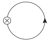
Figure 1: D01

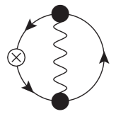
Figure 2: D02

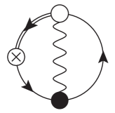
Figure 3: D03

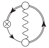
Figure 4: D04

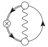
Figure 5: D05

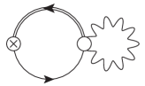
Figure 6: D06

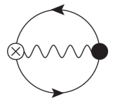
Figure 7: D07

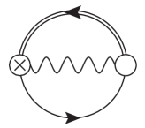
Figure 8: D08

Table 1: Contribution of each diagram to Eq. (2.14) in the unit of $\frac{-2\dim(R)N_{f}}{(4\pi)^{2}t^{2}}\frac{g_{0}^{2}}{(4\pi)^{2}}C_{2}(R)$.

diagram
D02	$-\dfrac{1}{\epsilon}-2\ln(8\pi t)+O(m_{0}^{2}t)$
D03	$2\dfrac{1}{\epsilon}+4\ln(8\pi t)+2+4\ln 2-2\ln 3+O(m_{0}^{2}t)$
D04	$-20\ln 2+16\ln 3+O(m_{0}^{2}t)$
D05	$12\ln 2-5\ln 3+O(m_{0}^{2}t)$
D06	$-4\dfrac{1}{\epsilon}-8\ln(8\pi t)-2+O(m_{0}^{2}t)$
D07	$8\ln 2-4\ln 3+O(m_{0}^{2}t)$
D08	$-2\ln 3+O(m_{0}^{2}t)$

The next to leading order expression for the expectation value (2.10) is given by the flow Feynman diagrams in Figs. 4–8 (and diagrams with arrows with the opposite direction). See Ref. Makino:2014taa for our convention for flow Feynman diagrams. These diagrams can be evaluated in a similar manner as Appendix B of Ref. Luscher:2010iy and the contribution of each diagram is tabulated in Table 1. Totally, we have

$$\left\langle\bar{\chi}(t,x)\overleftrightarrow{{\ooalign{\hfil/\hfil\crcr$D$}}}\chi(t,x)\right\rangle$$ (2.13)

$$=\frac{-2\dim(R)N_{f}}{(4\pi)^{2}t^{2}}\left\{(8\pi t)^{\epsilon}+\frac{g_{0}^{2}}{(4\pi)^{2}}C_{2}(R)\left[-3\frac{1}{\epsilon}-6\ln(8\pi t)+\ln(432)\right]+O(m_{0}^{2}t)+O(g_{0}^{4})\right\}.$$ (2.14)

Recalling the bare gauge coupling $g_{0}$ and the renormalized gauge coupling $g$ are related as $g_{0}^{2}=\mu^{2\epsilon}g^{2}[1+O(g^{2})]$, we see that the normalization factor in Eqs. (2.5) and (2.8) is given by

$$\frac{-2\dim(R)N_{f}}{(4\pi)^{2}t^{2}\left\langle\bar{\chi}(t,x)\overleftrightarrow{{\ooalign{\hfil/\hfil\crcr$D$}}}\chi(t,x)\right\rangle}=Z(\epsilon)\left\{1+\frac{g^{2}}{(4\pi)^{2}}C_{2}(R)\left[3\frac{1}{\epsilon}-\Phi(t)\right]+O(m^{2}t)+O(g^{4})\right\},$$ (2.15)

where

$$Z(\epsilon)\equiv\frac{1}{(8\pi t)^{\epsilon}},$$ (2.16)

and

$$\Phi(t)\equiv-3\ln(8\pi\mu^{2}t)+\ln(432).$$ (2.17)

Comparison of Eq. (2.15) with Eq. (3.24) of Ref. Makino:2014taa shows that the change from the hatted fermion variables in Ref. Makino:2014taa and to the present ringed fermion variables (2.5) and (2.8) entails the following changes in the expressions of Ref. Makino:2014taa :

$$z(\epsilon)\to Z(\epsilon),\qquad\phi\to\Phi(t).$$ (2.18)

2.2 Operator basis and the small flow-time expansion

To express the energy–momentum tensor in terms of local products of flowed fields, we introduce following five combinations which are even under the CP transformation,

$$\tilde{\mathcal{O}}_{1\mu\nu}(t,x) \equiv G_{\mu\rho}^{a}(t,x)G_{\nu\rho}^{a}(t,x),$$ (2.19)

$$\tilde{\mathcal{O}}_{2\mu\nu}(t,x) \equiv\delta_{\mu\nu}G_{\rho\sigma}^{a}(t,x)G_{\rho\sigma}^{a}(t,x),$$ (2.20)

$$\tilde{\mathcal{O}}_{3\mu\nu}(t,x) \equiv\mathring{\bar{\chi}}(t,x)\left(\gamma_{\mu}\overleftrightarrow{D}_{\nu}+\gamma_{\nu}\overleftrightarrow{D}_{\mu}\right)\mathring{\chi}(t,x),$$ (2.21)

$$\tilde{\mathcal{O}}_{4\mu\nu}(t,x) \equiv\delta_{\mu\nu}\mathring{\bar{\chi}}(t,x)\overleftrightarrow{{\ooalign{\hfil/\hfil\crcr$D$}}}\mathring{\chi}(t,x),$$ (2.24)

$$\tilde{\mathcal{O}}_{5\mu\nu}(t,x) \equiv\delta_{\mu\nu}m\mathring{\bar{\chi}}(t,x)\mathring{\chi}(t,x),$$ (2.25)

where $G_{\mu\nu}^{a}(t,x)$ is the field strength of the flowed gauge field. Because of the UV finiteness of the gradient flow Luscher:2011bx ; Luscher:2013cpa , these local products are finite when expressed in terms of renormalized parameters.

We introduce also corresponding bare operators in the $D$-dimensional $x$-space:

$$\mathcal{O}_{1\mu\nu}(x) \equiv F_{\mu\rho}^{a}(x)F_{\nu\rho}^{a}(x),$$ (2.26)

$$\mathcal{O}_{2\mu\nu}(x) \equiv\delta_{\mu\nu}F_{\rho\sigma}^{a}(x)F_{\rho\sigma}^{a}(x),$$ (2.27)

$$\mathcal{O}_{3\mu\nu}(x) \equiv\bar{\psi}(x)\left(\gamma_{\mu}\overleftrightarrow{D}_{\nu}+\gamma_{\nu}\overleftrightarrow{D}_{\mu}\right)\psi(x),$$ (2.28)

$$\mathcal{O}_{4\mu\nu}(x) \equiv\delta_{\mu\nu}\bar{\psi}(x)\overleftrightarrow{{\ooalign{\hfil/\hfil\crcr$D$}}}\psi(x),$$ (2.31)

$$\mathcal{O}_{5\mu\nu}(x) \equiv\delta_{\mu\nu}m_{0}\bar{\psi}(x)\psi(x).$$ (2.32)

We then expect that, according to the general argument Luscher:2011bx , the following asymptotic expansion for $t\to 0$ holds

$$\tilde{\mathcal{O}}_{i\mu\nu}(t,x)=\left\langle\tilde{\mathcal{O}}_{i\mu\nu}(t,x)\right\rangle+\zeta_{ij}(t)\left[\mathcal{O}_{j\mu\nu}(x)-\left\langle\mathcal{O}_{j\mu\nu}(x)\right\rangle\right]+O(t).$$ (2.33)

Once the mixing coefficients $\zeta_{ij}(t)$ in this expression are known, one may invert this relation up to $O(t)$ terms and express the energy-momentum tensor in the dimensional regularization

$$\left\{T_{\mu\nu}\right\}_{R}(x) =\frac{1}{g_{0}^{2}}\left\{\mathcal{O}_{1\mu\nu}(x)-\left\langle\mathcal{O}_{1\mu\nu}(x)\right\rangle-\frac{1}{4}\left[\mathcal{O}_{2\mu\nu}(x)-\left\langle\mathcal{O}_{2\mu\nu}(x)\right\rangle\right]\right\}$$

$$\qquad{}+\frac{1}{4}\left[\mathcal{O}_{3\mu\nu}(x)-\left\langle\mathcal{O}_{3\mu\nu}(x)\right\rangle\right]-\frac{1}{2}\left[\mathcal{O}_{4\mu\nu}(x)-\left\langle\mathcal{O}_{4\mu\nu}(x)\right\rangle\right]$$

$$\qquad\qquad{}-\left[\mathcal{O}_{5\mu\nu}(x)-\left\langle\mathcal{O}_{5\mu\nu}(x)\right\rangle\right],$$ (2.34)

in terms of the local products in Eqs. (2.19)–(2.25). The resulting expression will be

$$\left\{T_{\mu\nu}\right\}_{R}(x) =c_{1}(t)\left[\tilde{\mathcal{O}}_{1\mu\nu}(t,x)-\frac{1}{4}\tilde{\mathcal{O}}_{2\mu\nu}(t,x)\right]$$

$$\qquad{}+c_{2}(t)\left[\tilde{\mathcal{O}}_{2\mu\nu}(t,x)-\left\langle\tilde{\mathcal{O}}_{2\mu\nu}(t,x)\right\rangle\right]$$

$$\qquad\qquad{}+c_{3}(t)\left[\tilde{\mathcal{O}}_{3\mu\nu}(t,x)-2\tilde{\mathcal{O}}_{4\mu\nu}(t,x)-\left\langle\tilde{\mathcal{O}}_{3\mu\nu}(t,x)-2\tilde{\mathcal{O}}_{4\mu\nu}(t,x)\right\rangle\right]$$

$$\qquad\qquad\qquad{}+c_{4}(t)\left[\tilde{\mathcal{O}}_{4\mu\nu}(t,x)-\left\langle\tilde{\mathcal{O}}_{4\mu\nu}(t,x)\right\rangle\right]$$

$$\qquad\qquad\qquad\qquad{}+c_{5}(t)\left[\tilde{\mathcal{O}}_{5\mu\nu}(t,x)-\left\langle\tilde{\mathcal{O}}_{5\mu\nu}(t,x)\right\rangle\right]+O(t).$$ (2.35)

Eq. (2.35) shows that the energy–momentum tensor can be obtained as the $t\to 0$ limit of the combination in the right-hand side. Since the UV finite composite operators (2.19)–(2.25) should be independent of the regularization adopted, one may use the lattice regularization to compute correlation functions of the quantity in the right-hand side of Eq. (2.35). This provides a possible method to compute correlation functions of the correctly-normalized conserved energy–momentum tensor with the lattice regularization Suzuki:2013gza ; Makino:2014taa .

In Ref. Makino:2014taa , by using the hatted variables (2.2), the mixing coefficients $\zeta_{ij}(t)$ in Eq. (2.33) and the corresponding coefficients $c_{i}(t)$ in Eq. (2.35) were computed in the perturbation theory to the one-loop order. This perturbative computation is justified for $t\to 0$ by a renormalization group argument (see below). Fortunately, we do not need to repeat this computation anew for the present ringed variables (2.5) and (2.8); the only difference is the normalization of the fermion variables which amounts to the changes in Eq. (2.18). Making these changes in Eqs. (4.62)–(4.66) of Ref. Makino:2014taa , we have

$$c_{1}(t) =\frac{1}{g^{2}}-b_{0}\ln(8\pi\mu^{2}t)-\frac{7}{8}\frac{1}{(4\pi)^{2}}\left[\frac{11}{3}C_{2}(G)-\frac{12}{7}T(R)N_{f}\right],$$ (2.36)

$$c_{2}(t) =\frac{1}{8}\frac{1}{(4\pi)^{2}}\left[\frac{11}{3}C_{2}(G)+\frac{11}{3}T(R)N_{f}\right],$$ (2.37)

$$c_{3}(t) =\frac{1}{4}\left\{1+\frac{g^{2}}{(4\pi)^{2}}C_{2}(R)\left[\frac{3}{2}+\ln(432)\right]\right\},$$ (2.38)

$$c_{4}(t) =\frac{1}{8}d_{0}g^{2},$$ (2.39)

$$c_{5}(t) =-\left\{1+\frac{g^{2}}{(4\pi)^{2}}C_{2}(R)\left[3\ln(8\pi\mu^{2}t)+\frac{7}{2}+\ln(432)\right]\right\},$$ (2.40)

where the MS scheme is assumed and

$$b_{0}=\frac{1}{(4\pi)^{2}}\left[\frac{11}{3}C_{2}(G)-\frac{4}{3}T(R)N_{f}\right],\qquad d_{0}=\frac{1}{(4\pi)^{2}}6C_{2}(R).$$ (2.41)

2.3 Renormalization group argument

The use of the perturbation theory in computing $c_{i}(t)$ for $t\to 0$ is justified by the renormalization group argument. We apply

$$\left(\mu\frac{\partial}{\partial\mu}\right)_{0},$$ (2.42)

to both sides of Eq. (2.35), where $\mu$ is the renormalization scale and the subscript $0$ implies that the derivative is taken while all bare quantities are kept fixed. Since the energy–momentum tensor is not multiplicatively renormalized, $(\mu\partial/\partial\mu)_{0}(\text{left-hand side of Eq.~{}\eqref{eq:(2.24)}})=0$. On the right-hand side, since $\tilde{\mathcal{O}}_{1,2,3,4\mu\nu}(t,x)$ and $(1/m)\tilde{\mathcal{O}}_{5\mu\nu}(t,x)$ in Eqs. (2.19)–(2.25) are entirely given by bare quantities through the flow equations in Refs. Luscher:2010iy ; Luscher:2011bx ; Luscher:2013cpa , we have

$$\left(\mu\frac{\partial}{\partial\mu}\right)_{0}\tilde{\mathcal{O}}_{1,2,3,4\mu\nu}(t,x)=\left(\mu\frac{\partial}{\partial\mu}\right)_{0}\frac{1}{m}\tilde{\mathcal{O}}_{5\mu\nu}(t,x)=0.$$ (2.43)

These observations imply,

$$\left(\mu\frac{\partial}{\partial\mu}\right)_{0}c_{1,2,3,4}(t)=\left(\mu\frac{\partial}{\partial\mu}\right)_{0}mc_{5}(t)=0.$$ (2.44)

Then the standard renormalization group argument tells that $c_{1,2,3,4}(t)$ and $mc_{5}(t)$ are independent of the renormalization scale, if the renormalized parameters in these quantities are replaced by running parameters defined by

$$q\frac{d\bar{g}(q)}{dq}=\beta(\bar{g}(q)),\qquad\bar{g}(q=\mu)=g,$$ (2.45)

$$q\frac{d\bar{m}(q)}{dq}=-\gamma_{m}(\bar{g}(q))\bar{m}(q),\qquad\bar{m}(q=\mu)=m,$$ (2.46)

where $\mu$ is the original renormalization scale. Thus, since $c_{1,2,3,4}(t)$ and $mc_{5}(t)$ are independent of the renormalization scale, two possible choices, $q=\mu$ and $q=1/\sqrt{8t}$, should give an identical result. In this way, we have

$$c_{1,2,3,4}(t)(g,m;\mu) =c_{1,2,3,4}(t)(\bar{g}(1/\sqrt{8t}),\bar{m}(1/\sqrt{8t});1/\sqrt{8t}),$$ (2.47)

$$c_{5}(t)(g,m;\mu) =\frac{\bar{m}(1/\sqrt{8t})}{m}c_{5}(t)(\bar{g}(1/\sqrt{8t}),\bar{m}(1/\sqrt{8t});1/\sqrt{8t}),$$ (2.48)

where we have explicitly written dependence of $c_{i}(t)$ on renormalized parameters and on the renormalization scale. Finally, since the running gauge coupling $\bar{g}(1/\sqrt{8t})\to 0$ for $t\to 0$ thanks to the asymptotic freedom, we infer that we can compute $c_{i}(t)$ for $t\to 0$ by using the perturbation theory.

Applying Eqs. (2.47) and (2.48) to Eqs. (2.36)–(2.40), we have

$$c_{1}(t) =\frac{1}{\bar{g}(1/\sqrt{8t})^{2}}-b_{0}\ln\pi-\frac{7}{8}\frac{1}{(4\pi)^{2}}\left[\frac{11}{3}C_{2}(G)-\frac{12}{7}T(R)N_{f}\right],$$ (2.49)

$$c_{2}(t) =\frac{1}{8}\frac{1}{(4\pi)^{2}}\left[\frac{11}{3}C_{2}(G)+\frac{11}{3}T(R)N_{f}\right],$$ (2.50)

$$c_{3}(t) =\frac{1}{4}\left\{1+\frac{\bar{g}(1/\sqrt{8t})^{2}}{(4\pi)^{2}}C_{2}(R)\left[\frac{3}{2}+\ln(432)\right]\right\},$$ (2.51)

$$c_{4}(t) =\frac{1}{8}d_{0}\bar{g}(1/\sqrt{8t})^{2},$$ (2.52)

$$c_{5}(t) =-\frac{\bar{m}(1/\sqrt{8t})}{m}\left\{1+\frac{\bar{g}(1/\sqrt{8t})^{2}}{(4\pi)^{2}}C_{2}(R)\left[3\ln\pi+\frac{7}{2}+\ln(432)\right]\right\}.$$ (2.53)

The above expressions are for the MS scheme. The expressions in the $\overline{\text{MS}}$ scheme can be obtained by making the replacement

$$\ln\pi\to\gamma_{E}-2\ln 2,$$ (2.54)

in the above expressions.

This completes our construction of the lattice energy–momentum tensor in a new simpler prescription, which is expected to be free from a possible singularity accosiated with the massless fermion. The energy–momentum tensor is given by the $t\to 0$ limit of the right-hand side of Eq. (2.35), where the coefficients $c_{i}(t)$ are given by Eqs. (2.49)–(2.53); for the massless fermion, we can simply set $c_{5}(t)=0$ or discard the operator $\tilde{\mathcal{O}}_{5\mu\nu}(t,x)$. One may use any lattice transcription of operators (2.19)–(2.25) because these operators are UV finite. Note that coefficients (2.49)–(2.53) are universal in the sense that they are common for any lattice action and for any lattice transcription of operators (2.19)–(2.25) (as far as the classical continuum limit of the flow equations are identical to those of Refs. Luscher:2010iy ; Luscher:2011bx ; Luscher:2013cpa ). To utilize this “universality”, however, one has to take the continuum limit before the $t\to 0$ limit for Eq. (2.35). Practically, with a finite lattice spacing $a$, the flow time $t$ cannot be taken arbitrarily small because of a natural constraint,

$$a\ll\sqrt{8t}\ll R,$$ (2.55)

where $R$ denotes a typical low-energy scale. The extrapolation for $t\to 0$ thus generally requires a sufficiently fine lattice. The application to the thermodynamics of the quenched QCD Asakawa:2013laa strongly indicates that a reliable extrapolation to $t\to 0$ is feasible even with presently-available lattice parameters.

The work of H. S. is supported in part by a Grant-in-Aid for Scientific Research 23540330.

References

- (1) S. Caracciolo, G. Curci, P. Menotti and A. Pelissetto, Nucl. Phys. B 309, 612 (1988).
- (2) S. Caracciolo, G. Curci, P. Menotti and A. Pelissetto, Annals Phys. 197, 119 (1990).
- (3) H. Suzuki, PTEP 2013, no. 8, 083B03 (2013) [arXiv:1304.0533 [hep-lat]].
- (4) H. Makino and H. Suzuki, arXiv:1403.4772 [hep-lat].
- (5) M. Lüscher, JHEP 1008, 071 (2010) [arXiv:1006.4518 [hep-lat]].
- (6) M. Lüscher and P. Weisz, JHEP 1102, 051 (2011) [arXiv:1101.0963 [hep-th]].
- (7) M. Lüscher, JHEP 1304, 123 (2013) [arXiv:1302.5246 [hep-lat]].
- (8) L. Del Debbio, A. Patella and A. Rago, JHEP 1311, 212 (2013) [arXiv:1306.1173 [hep-th]].
- (9) M. Asakawa et al. [FlowQCD Collaboration], arXiv:1312.7492 [hep-lat].
- (10) D. Z. Freedman, I. J. Muzinich and E. J. Weinberg, Annals Phys. 87, 95 (1974).
- (11) S. D. Joglekar, Annals Phys. 100, 395 (1976) [Erratum-ibid. 102, 594 (1976)].
- (12) E. Itou, arXiv:1311.2676 [hep-lat].