Effects of Screening on Propagation of Graphene Surface Plasmons

Abstract

Electromagnetic fields bound tightly to charge carriers in a two-dimensional sheet, namely surface plasmons, are shielded by metallic plates that are a part of a device. It is shown that for epitaxial graphenes, the propagation velocity of surface plasmons is suppressed significantly through a partial screening of the electron charge by the interface states. On the basis of analytical calculations of the electron lifetime determined by the screened Coulomb interaction, we show that the screening effect gives results in agreement with those of a recent experiment.

Plasmons, which consist of carriers and electromagnetic fields, are the principal elements of excited states in solids. Mahan (2000) When carriers are confined in a two-dimensional layer, surface plasmons can exist. The electromagnetic fields appear outside the layer and can be sensitive to the screening effect provided, for example, by a metallic plate that is a part of a device, Ando (1982) which is not so obvious for other excited states in solids, such as electrons and phonons. A device composed of a two-dimensional sheet of carbons, graphene, Novoselov et al. (2005); Zhang et al. (2005) provides a great opportunity to study this sensitivity of surface plasmons, as was demonstrated by a recent time-resolved experiment, which we review below.

Figure 1(a) is the schematic of a transport experiment performed by Kumada et al on graphene grown by SiC sublimation. Kumada et al. (2014) After applying a current pulse with a frequency of a few GHz at the injection gate on epitaxial graphene, they observed the current induced at the detection gate located approximately 220 $\mu m$ from the injection gate. Figure 1(b) shows an example of the current observed as a function of time. The waveform has a peak structure at 1.5 ns, which enabled the authors to define the propagation velocity of a pulse as the propagation distance divided by the peak time, i.e., $220\mu m/1.5{\rm ns}\simeq 15\times 10^{4}$ m/s. The details of a waveform, such as peak time, depend on the Fermi energy position $E_{F}$, which was controlled using a metal top gate in their experiment. As a result, they were able to find the $E_{F}$ dependence of the velocity shown by the solid curve in Fig. 1(c). The velocity decreases as the Fermi energy approaches the Dirac point $E_{F}=0$ eV. For a wide range of $E_{F}$ the velocity is one order of magnitude smaller than the electron Fermi velocity $v_{F}\simeq 10^{6}$ m/s. Such a slow charge propagation in a gated graphene on SiC has been observed also for edge magnetoplasmons. Kumada et al. (2013) The velocity in a device without a top gate was observed to be one or two order of magnitude larger than $v_{F}$, suggesting that the presence/absence of the gate strongly affects the plasmon transport.

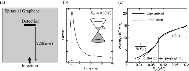
Figure 1: (a) Schematic of a time-resolved transport experiment on epitaxial graphene. Kumada et al. (2014) Because the experiments were performed at 1.5 K, the finite temperature effect Klimchitskaya et al. (2014) can be safely ignored. (b) The waveform of the current at the detection gate is given as a function of time. The details of the waveform are dependent on $E_{F}$, which is controlled by a metal top gate covering the entire sample. This plot corresponds to $E_{F}\simeq 0.2$ eV. (c) The $E_{F}$ dependence of the propagation velocity.

In this paper we provide a theoretical basis that is useful for studying the propagation velocity of surface plasmons in graphene, while paying particular attention to the effect of a metal gate on the transport properties.  We will show that in the absence of a metal gate, plasmons propagate faster than the electrons. In the presence of a metal gate, the propagation velocity is much slower than $v_{F}$ when the screening effect provided by interface states is taken into account. Furthermore, slow-moving surface plasmons undergo a strong diffusion when $E_{F}$ is near the Dirac point, which explains the drop at $E_{F}\simeq 0.1$ eV seen in Fig. 1(c).

We begin by showing that the group velocity of plasmons in graphene without a metal gate cannot be lower than $v_{F}/2$. The plasmon dispersion is derived from the zero value of the real part of the dielectric constant

$$\varepsilon_{E_{F}}(q,\omega)=1-v_{q}{\rm Re}\Pi_{E_{F}}(q,\omega)=0,$$ (1)

where $v_{q}$ is the Coulomb potential. Mahan (2000); Wunsch et al. (2006); Hwang and Das Sarma (2007) In the absence of a metal top gate, $v_{q}=2\pi e^{2}/\varepsilon q$, where $\varepsilon$ is the permittivity of a surrounding medium, $q$ is the wavevector magnitude, and $e$ is electron charge magnitude in vacuum ($e^{2}=1.44$ eV$\cdot$nm). $\Pi_{E_{F}}(q,\omega)$ is the polarization function, which is a function of $q$, frequency $\omega$, and $E_{F}$. Although the polarization function for doped graphene has been calculated in several papers, Wunsch et al. (2006); Hwang and Das Sarma (2007); Sasaki et al. (2012) we show it in Appendix A for clarity. Since $v_{q}>0$, the solution of Eq. (1) exists only when ${\rm Re}\Pi_{E_{F}}(q,\omega)>0$ is satisfied. It can be shown that ${\rm Re}\Pi_{E_{F}}(q,\omega)>0$ when $\omega>v_{F}q$ and ${\rm Re}\Pi_{E_{F}}(q,\omega)<0$ when $\omega<v_{F}q$, so that plasmons exist only when $\omega>v_{F}q$.  In the literature, $\omega<v_{F}q$ is referred to as an electron-hole continuum or an intraband single-particle excitation (or SPE_intra) region, where plasmons do not exist. When $\omega>v_{F}q$, ${\rm Re}\Pi_{E_{F}}(q,\omega)$ is approximated in the $q\to 0$ limit by

$${\rm Re}\Pi_{E_{F}}(q,\omega)\simeq\frac{|E_{F}|}{\pi}\left(\frac{q}{\hbar\omega}\right)^{2}.$$ (2)

On combining Eq. (1) with Eq. (2), we obtain the plasmon frequency Wunsch et al. (2006); Hwang and Das Sarma (2007)

$$\omega_{pl}(q,E_{F})=\frac{1}{\hbar}\sqrt{\frac{2e^{2}q|E_{F}|}{\varepsilon}}.$$ (3)

The $q$ dependence of $\omega_{pl}$, namely $\sqrt{q}$, is common to two-dimensional electron gas (2DEG) systems. Stern (1967) The existence of plasmons requires that the frequency satisfies

$$\omega_{pl}(q,E_{F})>v_{F}q.$$ (4)

Putting Eq. (3) into this condition, we have

$$\frac{1}{\hbar}\sqrt{\frac{2e^{2}|E_{F}|}{\varepsilon q}}>v_{F}.$$ (5)

Because the group velocity is defined by

$$v_{g}(q,E_{F})\equiv\frac{\partial\omega_{pl}(q,E_{F})}{\partial q}=\frac{1}{2\hbar}\sqrt{\frac{2e^{2}|E_{F}|}{\varepsilon q}},$$ (6)

it is shown that by combining Eq. (5) with Eq. (6) the plasmon group velocity has the lower limit

$$v_{g}(q,E_{F})>\frac{v_{F}}{2}.$$ (7)

This lower limit of the group velocity does not depend on $\varepsilon$, $q$, $E_{F}$, or $e^{2}$, whereas the factor $1/2$ reflects the exponent of $q$ in the dispersion relation. The solid line in Fig. 2 shows the lower limit. The actual group velocity must be located above the solid line, as indicated by the vertical arrow. It is also straightforward to show that the group velocity of an undamped plasmon will be located above the dashed curve (see Appendix B for details).

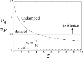
Figure 2: The lower limit of the group velocity of the plasmons in graphene without a nearby metal top gate. The plasmons cannot exist (are damped) when $v_{g}/v_{F}$ is located below the solid line (dashed curve). Screening lowers the dashed curve: the dotted curve is when $e_{*}=e/10$.

The conditions for the existence of plasmons and for plasmons to be undamped give the lower limit of the propagation velocity, while there is no condition that specifies the upper limit. This result suggests that the propagation velocity of the plasmons is generally high. For example, it is shown by eliminating $q$ from Eq. (6) using Eq. (3) that

$$v_{g}(\omega_{pl},E_{F})=\frac{e^{2}}{\hbar\varepsilon}\frac{|E_{F}|}{\hbar\omega_{pl}}.$$ (8)

When $\omega_{pl}=10$ GHz, $E_{F}=0.1$ eV, and $\varepsilon=10$, we have $v_{g}\simeq 6\times 10^{7}$ m/s.

When a metal plate is placed at a distance, $d$, from a graphene sheet as shown in Fig. 3(a), we have a metal-insulator-graphene device. Nakayama showed that surface plasmons exist for such a device. Nakayama (1974) The dispersion relation is given by

$$\omega_{s}(q)=\sqrt{\frac{2\pi\sigma_{0}\tau^{-1}}{\varepsilon}}\sqrt{\frac{q}{1+\coth(qd)}},$$ (9)

where $\sigma_{0}$ is the static conductivity and $\tau$ is the relaxation time.  In the absence of a metal gate (when $d\to\infty$), we can reproduce Eq. (3) from Eq. (9) using the Einstein relation, Ando (2008)

$$\sigma_{0}=e^{2}v_{F}^{2}\tau D(E_{F}),$$ (10)

where $D(E_{F})=2|E_{F}|/\pi(\hbar v_{F})^{2}$ is the density of states of graphene. Thus, Eq. (9) is a general result that includes Eq. (3) as the limiting case. In the presence of a metal gate, the $\sqrt{q}$-dependence is lost for long-wavelength modes (or when $q^{-1}\gg d$) and $\omega_{s}$ exhibits a linear dependence on $q$ as

$$\omega_{s}(q)=\sqrt{\frac{2\pi\sigma_{0}\tau^{-1}d}{\varepsilon}}q,\ \ (qd\ll 1).$$ (11)

Then the group velocity is given by

$$v\equiv\frac{\partial\omega_{s}(q)}{\partial q}=\sqrt{\frac{2\pi\sigma_{0}\tau^{-1}d}{\varepsilon}}.$$ (12)

The electric fields of surface plasmons have their principal component normal to the graphene sheet ${\bf E}=(0,0,E_{z})$, as shown in Fig. 3(a). This field configuration is obtained by solving Maxwell’s equations for electromagnetic fields (see Ref. Nakayama, 1974 for details). The field configuration is in sharp contrast to that in the absence of a top gate (when $d\to\infty$), where the electric fields have components both normal and parallel to the graphene sheet as ${\bf E}=(E_{x},0,E_{z})$ where $E_{x}(x,z,t)=Ee^{i(kx-\omega t)-\alpha|z|}$ and $E_{z}(x,z,t)=ikE_{x}(x,z;t)/\alpha$ with $\alpha\equiv\sqrt{k^{2}-\varepsilon\omega^{2}/c^{2}}$ (see Ref. Nakayama, 1974 for details). Because $d$ is 200 nm and the condition $qd\ll 1$ is satisfied in Ref. Kumada et al., 2014, the excitation described by Eq. (12) is considered to be that observed in the experiment in the presence of a metal top gate. However, the application of the Einstein relation Eq. (10) to Eq. (12) gives

$$v=\frac{e}{\hbar}\sqrt{\frac{4|E_{F}|d}{\varepsilon}}.$$ (13)

The velocity predicted from Eq. (13) with $\varepsilon=4$ and $d=200$ nm is $v=25\sqrt{|E_{F}|/{\rm eV}}\times 10^{6}$ m/s, which is two orders of magnitude larger than that observed in the experiment (see Fig. 1(c)).

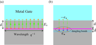
Figure 3: (color) Cross-section of a device consisting of a graphene sheet (red) and a metal gate (blue). The gray regions represent a dielectric (dielectric constant $\varepsilon$). (a) The arrows represent the electric fields ${\bf E}=(0,0,E_{z})$ for non-radiative (acoustic) plasmons satisfying $q^{-1}\gg d$. We omit to draw an exponential decaying electric field which appears underneath the graphene sheet for clarity. (b) Interface states near to graphene sheet, including the dangling bond states ($\delta\ll d$), efficiently screen the electron charge.

The discrepancy between the predicted and experimental values of velocity can be accounted for by a modification of the Einstein relation caused by a strong (but not perfect) screening effect produced by interface (trap) states. In an epitaxial graphene device grown on SiC, the interface states are naturally realized by the dangling bond states at the SiC substrate [see Fig. 3(b)]. Zebrev (2011); Takase et al. (2012) When the (positive) charge $e$ exists in the graphene sheet, a screening charge with approximately $-e$ is induced on the dangling bond states. Meanwhile, the screening effect of the interface states is not perfect, and a (positive) charge with magnitude $e_{*}$ remains in the capacitor consisting of the graphene sheet and dangling bond states, as shown schematically in Fig. 3(b). Luryi (1988) This charge induces (negative) screening charge with $-e_{*}$ on the metal top gate. If surface plasmons consist of particles with charge magnitude $e_{*}$, we can expect Eq. (10) to be defined by replacing $e$ with the screened charge $e_{*}$ as

$$\sigma_{0}=e_{*}^{2}v_{\rm F}^{2}\tau D(E_{F}).$$ (14)

The corrected velocity is given by the application of Eq. (14) to Eq. (12) as

$$v=\frac{e_{*}}{\hbar}\sqrt{\frac{4|E_{F}|d}{\varepsilon}}.$$ (15)

The value of $e_{*}$ can be roughly estimated by an extension of the result of Luryi, Luryi (1988) in which $e_{*}$ is expressed in terms of the quantum capacitance of the interface states $C_{i}$ [$=e^{2}\gamma$] and geometrical capacitance $C_{d}$ [$=\varepsilon/d$] as

$$e_{*}\simeq\frac{C_{d}}{C_{i}+C_{d}}e,$$ (16)

in the static limit. When we adopt the value $\gamma=0.37$ eV${}^{-1}\cdot$nm^-2 obtained by Takase et al., Takase et al. (2012) $e_{*}/e\simeq 0.036$ for $d=200$ nm and $\varepsilon=4$. This value is in agreement with the experiment.  The advantage of incorporating screening is that as long as the interface states near to graphene are taken into account through the modification of the Coulomb potential in Eq. (1) as

$$v_{q}=\frac{2\pi e_{*}^{2}}{q},$$ (17)

the conclusion obtained in the absence of a metal top gate is valid even in the presence of the interface states since the lower limit stems from the $\sqrt{q}$-dependence of $\omega_{p}$ and is independent of the electron charge as shown in Eq. (7). This result is also consistent with the experiment.

Propagation velocity can be suppressed by resistivity $R$, which is not taken into account in Eq. (15). To investigate the effect of $R$ on the propagation velocity, we can adopt an $RLC$ circuit model introduced by Burke et al. for studying plasmons in a 2DEG system. Burke et al. (2000) The use of this model was motivated by the fact that the electric fields in the dielectric shown in Fig. 3(b) are similar to those in a waveguide, for which the wave propagation is described by an $RLC$ circuit model. In this model, $C$ and $L$ correspond to $C_{d}$ and the kinetic inductance of graphene, respectively. In Ref. Kumada et al., 2014 we simulated the time evolution of the pulse using the Runge-Kutta method and obtained the waveform at the detector. By following the procedure used in the experiment, we determined the propagation velocity of the pulse in terms of the peak time and obtained the dashed curve in Fig. 1(c). Our simulation reproduces the experimental result satisfactorily. The effect of $R$ on the propagation velocity can be examined analytically in terms of the continuum approximation of the $RLC$ circuit model given by the telegrapher’s equation, Kumada et al. (2014); Doetsch (1971); Sonnenschein et al. (2000)

$$\left[\frac{\partial^{2}}{\partial t^{2}}-v^{2}\nabla^{2}+\frac{R}{L}\frac{\partial}{\partial t}\right]E_{z}({\bf r},t)=0,$$ (18)

where

$$v=\frac{1}{\sqrt{LC_{d}}},$$ (19)

and inductance $L$ is given from Eqs. (12) and (14) by

$$L=\frac{\tau}{2\pi\sigma_{0}}=\frac{1}{2\pi e_{*}^{2}v_{F}^{2}D(E_{F})}.$$ (20)

The solution may be constructed from the Green’s function of the Klein-Gordon equation,

$$\left[\frac{\partial^{2}}{\partial t^{2}}-v^{2}\nabla^{2}+m^{2}\right]\phi({\bf r},t)=0,$$ (21)

with a negative mass squared $m^{2}=-q_{c}^{2}v^{2}$ where $q_{c}$ is the damping factor,

$$q_{c}\equiv\frac{R}{2}\sqrt{\frac{C_{d}}{L}},$$ (22)

because the telegrapher’s equation is reproduced from the Klein-Gordon equation by setting $\phi({\bf r},t)=e^{q_{c}vt}E_{z}({\bf r},t)$. The retarded Green’s function of the Klein-Gordon equation is well-known and written as $\Delta_{R}({\bf r},t)=\theta(t)\Delta({\bf r},t)$ where

$$\Delta({\bf r},t)=\frac{{\rm sgn}(t)}{2\pi}\times$$

$$\left[\delta(t^{2}-\frac{|{\bf r}|^{2}}{v^{2}})-\frac{m}{2}\theta(t^{2}-\frac{|{\bf r}|^{2}}{v^{2}})\frac{J_{1}(m\sqrt{t^{2}-\frac{|{\bf r}|^{2}}{v^{2}}})}{\sqrt{t^{2}-\frac{|{\bf r}|^{2}}{v^{2}}}}\right],$$ (23)

and $J_{1}(x)$ is the Bessel function of the first kind. Thus, by specifying the initial condition $E_{z}(0,t)$, the solution of the telegrapher’s equation is written as $E_{z}(x,t)=E_{p}(x,t)+E_{d}(x,t)$ for $t>x/v$ where Doetsch (1971); Sonnenschein et al. (2000)

$$E_{p}(x,t)=e^{-q_{c}x}E_{z}(0,t-\frac{x}{v}),$$ (24)

$$E_{d}(x,t)=q_{c}x\int_{\frac{x}{v}}^{t}e^{-q_{c}vt^{\prime}}\frac{I_{1}(q_{c}v\sqrt{t^{\prime 2}-\frac{x^{2}}{v^{2}}})}{\sqrt{t^{\prime 2}-\frac{x^{2}}{v^{2}}}}E_{z}(0,t-t^{\prime})dt^{\prime}.$$ (25)

Here, we used $I_{1}(x)=-iJ_{1}(ix)$ where $I_{1}(z)$ is the modified Bessel function of the first kind. Here, $E_{p}(x,t)$ is an exponentially decaying signal that propagates at a speed $v$, and $E_{d}(x,t)$ expresses diffusion.

The effect of $R$ on the plasmon propagation is most clearly visualized at the drop in the peak velocity observed below $E_{F}\simeq 0.1$ eV in Fig. 1(c) which is due to the dominance of diffusion. For the $\delta$-function initial pulse $E_{z}(0,t)=\delta(t)$, it is shown that by differentiating Eqs. (24) and (25) with respect to $t$, the time $t^{*}$ corresponding to the peak in the waveform is $t^{*}=x/v$ for $E_{p}(x,t)$ and $t^{*}\approx q_{c}x^{2}/3v$ for $E_{d}(x,t\gg x/v)$. Sonnenschein et al. (2000) Thus, when $E_{p}$ dominates $E_{d}$ (propagation dominant), the peak velocity is given by $x/t^{*}=v$, on the other hand, when $E_{d}$ dominates $E_{p}$ (diffusion dominant) the peak velocity is suppressed by the factor of $3/q_{c}x$ as $x/t^{*}\approx 3v/q_{c}x$. Hence, when diffusion dominates, the peak velocity exhibits the $E_{F}$ dependence of $v/q_{c}$ ($\propto 1/R$), while when propagation dominates it exhibits the $v$ ($\propto\sqrt{|E_{F}|}$) dependence. Whether $E_{d}$ dominates $E_{p}$ can depend sensitively on the value of $q_{c}$. This should be examined for a more realistic initial pulse, namely for the Gaussian initial pulse $E_{z}(0,t)=\exp(-t^{2}/T^{2})$ where $T=400$ ps. Kumada et al. (2014) We plot $E_{p}(x,t)$, $E_{d}(x,t)$, and $E_{z}(x,t)$ at $x=220$ $\mu m$ for different $q_{c}$ values in Fig. 4. When $q_{c}=0$, the peak time is seen at $t^{*}=2.2$ ns, so the propagation velocity $x/t^{*}$ is $10^{5}$ m/s, which is approximately equal to the velocity at $E_{F}=0.1$ eV in Fig. 1(c). In Fig. 4, it is seen that when $q_{c}<0.1$, $E_{p}$ dominates $E_{d}$, whereas when $q_{c}>0.3$, $E_{d}$ dominates $E_{p}$. The maximum amplitudes of $E_{p}$ and $E_{d}$ are similar when $q_{c}\simeq 0.2$. The peak time $t^{*}$ increases rapidly when $q_{c}$ changes very slightly from 0.2 to 0.3. This means that the peak velocity decreases rapidly then, which can explain that the velocity decreases rapidly below $E_{F}\simeq 0.1$ eV in Fig. 1(c). Indeed, when we adopt the values obtained in Ref. Kumada et al., 2014: $R(E_{F})=340+3.7\times 10^{6}/(22+(500E_{F})^{2})$ $\Omega$ and $\sqrt{C_{d}/L}=\sqrt{0.58|E_{F}|}\times 10^{-3}$ $\Omega^{-1}$, $q_{c}$ changes from 0.218 to 0.283 when $E_{F}$ decreases a little from 0.1 to 0.08.

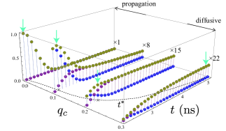
Figure 4: (color) The $q_{c}$-dependence of the waveform at $x=220$ $\mu m$. In this plot we assume $T=400$ ps and $v=10^{5}$ m/s, and $q_{c}$ is given in the units of $(10\mu m)^{-1}$. The peak time of the $E_{p}$ component (blue) is $t=2.2$ ns, while that of the $E_{d}$ component (red) increases with increasing $q_{c}$. The sum of the two components, $E_{z}$, is referred by yellow. Arrows represent peak time.

Since $E_{d}(x,t)$ is proportional to $q_{c}$, diffusion is suppressed by decreasing $q_{c}$, which may be realized by decreasing $R$ or increasing $L$ [see Eq. (22)]. Achieving a large $L$ (or small $R$) is also important in order to extend the relaxation time $\tau^{\prime}\equiv 1/(vq_{c})=2L/R$ or to suppress the damping caused by $\exp(-q_{c}vt)$ for $E_{p}(x,t)$. However, it should be noted that since both $L$ and $R$ decrease as $|E_{F}|$ increases, increasing $L$ by decreasing $|E_{F}|$ is incompatible with decreasing $R$. On the other hand, $L$ ($q_{c}$) is enhanced (suppressed) significantly by the screening effect provided by the interface states.

To conclude, the effects of a metal top gate and interface states on the plasmon transport have been revealed: the former provides linearly dispersed plasmons, while the latter renormalizes the effective charge. In the absence of a metal top gate, the propagation velocity of surface plasmons has a lower limit given by $v_{F}/2$. This lower limit is a rigid consequence derived from the condition for the existence of plasmons and independent of the electron charge in particular. Thus, as long as the interface states are taken into account as the origin of the partial screening effect (i.e., $v_{q}=2\pi e^{2}/q\to 2\pi e_{*}^{2}/q$), the conclusion is valid even in the presence of the interface states. In the presence of a metal top gate, the lower limit may be ineffective due to the modification of the dispersion relation of the surface plasmons ($\omega_{pg}\propto\sqrt{q}\to q$). For the linear dispersion, we could utilize the concept of inductance for analyzing the velocity. An analysis using the $RLC$ circuit model and telegrapher’s equation successfully explained the experimental results for the $E_{F}$ dependence of the propagation velocity, which proves that the inductance is effectively enhanced in the presence of a metal top gate. We attributed the enhancement to the screening effect induced by the interface states and found the idea to be consistent with the electron lifetime. A straightforward deduction from our results is that surface plasmons in a device consisting of exfoliated graphene without interface states experiences strong dumping and the propagation is severely suppressed. In other words, epitaxial graphenes have an advantage over exfoliated graphenes in realizing high inductance.

Appendix A Polarization function

In this appendix, we use $v$ for $v_{F}$ and $\mu$ for $E_{F}/\hbar$. The polarization function is given by

$$-{\rm Im}\Pi_{\mu}(q,\omega)=$$

$$\frac{1}{2\pi}\frac{(vq)^{2}}{\sqrt{\omega^{2}-(vq)^{2}}}\theta_{\omega-vq}\left[\theta_{\frac{\omega-vq}{2}-\mu}\left\{F(1)-F(-1)\right\}+\theta_{\mu-\frac{\omega-vq}{2}}\theta_{\frac{\omega+vq}{2}-\mu}\left\{F(1)-F\left(\frac{2\mu-\omega}{vq}\right)\right\}\right]+$$

$$\frac{1}{2\pi}\frac{(vq)^{2}}{\sqrt{(vq)^{2}-\omega^{2}}}\theta_{vq-\omega}\left[\theta_{\mu-\frac{vq-\omega}{2}}G\left(\frac{2\mu+\omega}{vq}\right)-\theta_{\mu-\frac{\omega+vq}{2}}G\left(\frac{2\mu-\omega}{vq}\right)\right]$$ (26)

$${\rm Re}\Pi_{\mu}(q,\omega)=-\frac{2\mu}{\pi}$$

$$-\frac{1}{2\pi}\frac{(vq)^{2}}{\sqrt{\omega^{2}-(vq)^{2}}}\theta_{\omega-vq}\left[\theta_{\frac{\omega-vq}{2}-\mu}G\left(\frac{\omega-2\mu}{vq}\right)+\theta_{\mu-\frac{\omega+vq}{2}}G\left(\frac{2\mu-\omega}{vq}\right)-G\left(\frac{\omega+2\mu}{vq}\right)\right]$$

$$-\frac{1}{2\pi}\frac{(vq)^{2}}{\sqrt{(vq)^{2}-\omega^{2}}}\theta_{vq-\omega}\left[\theta_{\frac{vq+\omega}{2}-\mu}\left\{F(1)-F\left(\frac{2\mu-\omega}{vq}\right)\right\}+\theta_{\frac{vq-\omega}{2}-\mu}\left\{F\left(1\right)-F\left(\frac{\omega+2\mu}{vq}\right)\right\}\right]$$ (27)

where $\theta_{x}$ denotes the step function satisfying $\theta_{x\geq 0}=1$ and $\theta_{x<0}=0$. The functions $F$ and $G$ are defined by

$$F(x)=\frac{1}{2}\left\{x\sqrt{1-x^{2}}+\sin^{-1}(x)\right\},$$ (28)

$$G(x)=\frac{1}{2}\left\{x\sqrt{x^{2}-1}-\ln\left(x+\sqrt{x^{2}-1}\right)\right\},$$ (29)

respectively. We showed a direct derivation of the above formula in Supplemental Material of Ref. Sasaki et al., 2012, for which we need to multiply $g_{v}/(2\pi\hbar v_{F})^{2}$ with $g_{v}=2$.

Appendix B

The dashed curve in Fig. 2 is based on the inequality given by

$$v_{p}(q,E_{F})>\frac{e}{2\hbar}\sqrt{\frac{\hbar v_{F}+\frac{e^{2}}{2\varepsilon}+\sqrt{\hbar v_{F}\frac{e^{2}}{\varepsilon}+\left(\frac{e^{2}}{2\varepsilon}\right)^{2}}}{\varepsilon}}.$$ (30)

This lower limit of the group velocity depends on the values of $\varepsilon$ and $e$. The dotted curve in Fig. 2 is the plot when $e$ is replaced with $e^{*}=e/10$.

Equation (30) arises from the fact that plasmons can decay into the constituent (interband) electron-hole pairs of the collective charge-density oscillations. The decay is suppressed (plasmons become undamped) when

$$|E_{F}|>\frac{\hbar\omega_{p}(q,E_{F})+\hbar v_{F}q}{2}$$ (31)

holds, otherwise the decay of plasmons into single particle electron-hole pairs is not negligibly small. Sasaki et al. (2012) Mathematically, Eq. (31) is equivalent to a condition where the imaginary part of the polarization function Eq. (26) vanishes: ${\rm Im}\Pi_{E_{F}}(q,\omega_{p}(q))=0$ for $\omega_{p}(q)>v_{F}q$. The condition of Eq. (30) can be obtained by putting Eq. (3) into Eq. (31) to obtain

$$|E_{F}|>\frac{q}{2}\left(\hbar v_{F}+\frac{e^{2}}{2\varepsilon}+\sqrt{\hbar v_{F}\frac{e^{2}}{\varepsilon}+\left(\frac{e^{2}}{2\varepsilon}\right)^{2}}\right),$$ (32)

and then by using Eq. (6).

Appendix C

When $\omega\equiv vq<v_{F}q$ (or $v<v_{F}$) and Eq. (31) is satisfied, the imaginary part of $\Pi_{E_{F}}(q,\omega)$ is written as

$$-{\rm Im}\Pi_{E_{F}}(q,\omega)=\frac{\hbar v_{F}q}{4\pi\sqrt{1-\frac{\omega^{2}}{(v_{F}q)^{2}}}}$$

$$\times\left\{G\left(\frac{2|E_{F}|+\hbar\omega}{\hbar v_{F}q}\right)-G\left(\frac{2|E_{F}|-\hbar\omega}{\hbar v_{F}q}\right)\right\},$$ (33)

where $G(x)\equiv\left\{x\sqrt{x^{2}-1}-\log\left(x+\sqrt{x^{2}-1}\right)\right\}/2$. Note that $dG(x)/dx=\sqrt{x^{2}-1}$. According to the time-energy uncertainly relation, the mean lifetime is approximated by

$$\tau\equiv-\frac{\hbar}{2{\rm Im}\Pi_{E_{F}}(q,\omega)}\simeq\frac{v_{F}}{v}\sqrt{1-\left(\frac{v}{v_{F}}\right)^{2}}\frac{\pi\hbar}{|E_{F}|}.$$ (34)

The characteristic time scale of $\tau$ is of the order of a femtosecond because $\tau\simeq 2.5\times 10^{-2}(v_{\rm F}/v)|\varepsilon_{\rm F}|^{-1}$ fs ($\varepsilon_{\rm F}$ is in units of eV), when $v\ll v_{F}$.

Appendix D

We examined the $d$ dependence of the electron’s quasi-particle lifetime determined by the Coulomb interaction to validate the assumption of screening. The lifetime is given by the inverse of the imaginary part of the electron selfenergy $\Sigma$ as $\tau_{q}=\hbar/2{\rm Im}\Sigma$. We calculated ${\rm Im}\Sigma$ using the formula, Quinn and Ferrell (1958); Hawrylak (1987); Das Sarma et al. (2007)

$${\rm Im}\Sigma_{\bf k}(E_{F}>0)=\int\frac{d^{2}{\bf k^{\prime}}}{(2\pi)^{2}}\left\{\theta(\xi_{\bf k}-\xi_{\bf k^{\prime}})-\theta(\xi_{\bf k^{\prime}}-E_{F})\right\}$$

$$\times\frac{1+\cos\left(\Theta_{\bf k^{\prime}}-\Theta_{\bf k}\right)}{2}{\rm Im}\frac{v_{|{\bf k^{\prime}}-{\bf k}|}}{\varepsilon_{E_{F}}(|{\bf k^{\prime}}-{\bf k}|,\xi_{\bf k}-\xi_{\bf k^{\prime}})},$$ (35)

where $\xi_{\bf k}=\hbar v_{F}|{\bf k}|$, $k_{x}-ik_{y}=|{\bf k}|\exp(-i\Theta_{\bf k})$, and $v_{q}$ denotes the screened Coulomb potential given by

$$v_{q}=\frac{4\pi e_{*}^{2}}{\varepsilon q(1+\coth(qd))}.$$ (36)

Note that Eq. (15) may be obtained from Eq. (1) with this $v_{q}$. Principi et al. (2011) A straightforward calculation shows that when $\xi_{k}\simeq E_{F}$, ${\rm Im}\Sigma_{\bf k}(E_{F}>0)$ is approximated by $\hbar v_{F}|\xi_{k}-E_{F}|/(16E_{F}d)$.  As a result, we obtain

$$\tau_{q}=\frac{8E_{F}d}{v_{F}|\xi_{k}-E_{F}|}.$$ (37)

Here let us assume that $\tau_{q}$ is longer than the peak time ($t^{*}$). When $|\xi_{k}-E_{F}|=10$ GHz and $d=200$ nm, $\tau_{q}$ is of the order of ns, which is consistent with the experimental result shown in Fig. 1(b), where the electron peak time is of the order of ns, at least. If $d=1$ nm, $\tau_{q}$ shortens as ${\cal O}({\rm ps})$ and is inconsistent with the experiment. Since $\tau_{q}$ is independent of the charge, a unique solution for explaining $v\ll v_{F}$ is to assume $e_{*}$ (instead of $e$) as shown in Eq. (36) and use Eq. (36) with Eq. (1).

We note that $t^{*}$ should not be identified with the transport relaxation time ($\tau$), which is estimated from the mobility $\mu$ using $\mu=e_{*}\tau/m$ where the effective mass $m$ satisfies $mv_{F}^{2}/2=|E_{F}|$. Because, when $E_{F}=0.1$ eV, $\mu\simeq 5000$ cm²/V$\cdot$s is the typical value for epitaxial graphene samples, Takase et al. (2012) $\tau$ is the order of picoseconds. This result is not in good agreement with the experiment showing that $t^{*}$ is the order of nanoseconds. Even though the Coulomb (electron-electron) interaction provides a finite quasi-particle lifetime, it does not contribute to the transport time. We also note that the plasmon lifetime determined by the Coulomb interaction is estimated in Refs. Principi et al., 2013 and Principi et al., 2013.

References

- Mahan (2000) G. D. Mahan, Many-Particle Physics (Springer, 2000).
- Ando (1982) T. Ando, Reviews of Modern Physics, 54, 437 (1982), ISSN 0034-6861.
- Novoselov et al. (2005) K. S. Novoselov, A. K. Geim, S. V. Morozov, D. Jiang, M. I. Katsnelson, I. V. Grigorieva, S. V. Dubonos, and A. A. Firsov, Nature, 438, 197 (2005).
- Zhang et al. (2005) Y. Zhang, Y.-W. Tan, H. L. Stormer, and P. Kim, Nature, 438, 201 (2005).
- Kumada et al. (2014) N. Kumada, R. Dubourget, K. Sasaki, S. Tanabe, H. Hibino, H. Kamata, M. Hashisaka, K. Muraki, and T. Fujisawa, New Journal of Physics, 16, 063055 (2014), ISSN 1367-2630.
- Kumada et al. (2013) N. Kumada, S. Tanabe, H. Hibino, H. Kamata, M. Hashisaka, K. Muraki, and T. Fujisawa, Nature communications, 4, 1363 (2013), ISSN 2041-1723.
- Klimchitskaya et al. (2014) G. L. Klimchitskaya, V. M. Mostepanenko, and B. E. Sernelius, Physical Review B, 89, 125407 (2014), ISSN 1098-0121.
- Wunsch et al. (2006) B. Wunsch, T. Stauber, F. Sols, and F. Guinea, New Journal of Physics, 8, 318 (2006), ISSN 1367-2630.
- Hwang and Das Sarma (2007) E. H. Hwang and S. Das Sarma, Physical Review B, 75, 205418 (2007), ISSN 1098-0121.
- Sasaki et al. (2012) K.-i. Sasaki, K. Kato, Y. Tokura, S. Suzuki, and T. Sogawa, Phys. Rev. B, 86, 201403 (2012).
- Stern (1967) F. Stern, Physical Review Letters, 18, 546 (1967), ISSN 0031-9007.
- Nakayama (1974) M. Nakayama, J. Phys. Soc. Jpn., 36, 393 (1974).
- Ando (2008) T. Ando, Progress of Theoretical Physics Supplement, 176, 203 (2008), ISSN 0375-9687.
- Zebrev (2011) G. Zebrev, in Physics and Applications of Graphene - Theory, edited by S. Mikhailov (InTech, 2011) p. 475.
- Takase et al. (2012) K. Takase, S. Tanabe, S. Sasaki, H. Hibino, and K. Muraki, Phys. Rev. B, 86, 165435 (2012).
- Luryi (1988) S. Luryi, Applied Physics Letters, 52, 501 (1988), ISSN 00036951.
- Burke et al. (2000) P. J. Burke, I. B. Spielman, J. P. Eisenstein, L. N. Pfeiffer, and K. W. West, Appl. Phys. Lett., 76, 745 (2000).
- Doetsch (1971) G. Doetsch, Guide to the applications of the Laplace and Z-transforms (Reinhold, 1971).
- Sonnenschein et al. (2000) E. Sonnenschein, I. Rutkevich, and D. Censor, Progress In Electromagnetics Research, 27, 129 (2000).
- Quinn and Ferrell (1958) J. Quinn and R. Ferrell, Physical Review, 112, 812 (1958), ISSN 0031-899X.
- Hawrylak (1987) P. Hawrylak, Physical Review Letters, 59, 485 (1987), ISSN 0031-9007.
- Das Sarma et al. (2007) S. Das Sarma, E. Hwang, and W.-K. Tse, Physical Review B, 75, 121406 (2007), ISSN 1098-0121.
- Principi et al. (2011) A. Principi, R. Asgari, and M. Polini, Solid State Communications, 151, 1627 (2011), ISSN 00381098.
- Principi et al. (2013) A. Principi, G. Vignale, M. Carrega, and M. Polini, Physical Review B, 88, 121405 (2013a), ISSN 1098-0121.
- Principi et al. (2013) A. Principi, G. Vignale, M. Carrega, and M. Polini, Physical Review B, 88, 195405 (2013b), ISSN 1098-0121.
- Mikhailov and Ziegler (2007) S. Mikhailov and K. Ziegler, Physical Review Letters, 99, 016803 (2007), ISSN 0031-9007.
- Bordag and Pirozhenko (2014) M. Bordag and I. G. Pirozhenko, Physical Review B, 89, 035421 (2014), ISSN 1098-0121.
- Allen (1997) P. B. Allen, From Quantum Mechanics to Technology, edited by Z. Petru, J. Przystawa, and K. Rapcewicz, Lecture Notes in Physics, Vol. 477 (Springer Berlin Heidelberg, 1997) ISBN 978-3-540-61792-1, pp. 125–141.