Abstract

The conjecture that some unknown symmetry is responsible for keeping the Higgs boson light at 125 GeV does not hold for the Standard Model, where the coefficient of the quadratic divergence of Higgs boson self-energy is far from zero. We show that such a cancellation can be achieved in two-Higgs doublet models, by virtue of which all the scalars remain at the electroweak scale and the naturalness problem is avoided. We explore the consequences of such cancellations in different two-Higgs doublet models with no flavour-changing neutral current, and show that the parameter space becomes tightly constrained; in particular, the ratio of two vacuum expectation values, $\tan\beta$, no longer remains a free parameter but turns out to be a function of the quartic couplings.

PACS no.: 12.60.Fr, 14.80.Ec

1 Introduction

The two-Higgs doublet models (2HDM) [1] are one of the most widely investigated scenarios that go beyond the Standard Model (SM). Any 2HDM consists of five physical scalars: two CP-even neutral $h$ and $H$, one CP-odd neutral $A$, and two charged bosons $H^{\pm}$. The CP quantum numbers are, of course, assigned with the assumption that the scalar potential is CP conserving and hence the mass eigenstates are also CP eigenstates. However, a generic 2HDM suffers from large flavour-changing neutral currents (FCNC); to prevent this, one invokes the Glashow-Weinberg-Paschos theorem [2, 3]. The theorem states that there will be no tree-level FCNC if all right-handed fermions of a given electric charge couple to only one of the doublets. This can be achieved in 2HDMs by introducing discrete symmetries for fermions or scalars.

Let us denote the two doublets by $\Phi_{1}$ and $\Phi_{2}$, and invoke a $Z_{2}$ symmetry $\Phi_{1}\to-\Phi_{1}$, $\Phi_{2}\to\Phi_{2}$. There are four types of 2HDM, depending on the transformation of the fermions under this $Z_{2}$, for which there will be no tree-level FCNC. They are: (i) Type I, for which all fermions couple with $\Phi_{2}$ and none with $\Phi_{1}$; (ii) Type II, for which up-type quarks couple to $\Phi_{2}$ and down-type quarks and charged leptons couple to $\Phi_{1}$ (this is the type that is embedded in the minimal supersymmetric SM (MSSM) and hence has received the most attention); (iii) Type Y (sometimes called Type III or Flipped), for which up-type quarks and charged leptons couple to $\Phi_{2}$ and down-type quarks couple to $\Phi_{1}$, and (iv) Type X (sometimes called Type IV or Lepton-specific), for which all charged leptons couple to $\Phi_{1}$ and all quarks couple to $\Phi_{2}$. Apart from these four, there are other 2HDMS with tree-level FCNC which can be kept under control [4] and which lead to interesting phenomenology [5, 6] which we will not pursue in this paper.

The facts that the SM can be an effective theory valid all the way up to the Planck scale ($M_{Pl}=1/\sqrt{G_{N}}\sim 10^{19}$ GeV) and there is no symmetry protecting the scalar masses lead to the naturalness problem: why the Higgs boson mass is of the order of the electroweak scale and not driven by the radiative corrections to the Planck scale. As we do not yet know, from experiments, of any symmetry that can protect the scalar mass, we will take a bottom-up approach, first suggested by Veltman [7], that due to some yet-to-be-discovered symmetry, the radiative corrections to the scalar mass either vanish or are kept at a manageable level. This is popularly known as the Veltman condition (VC).

The Veltman condition is not an anthropic principle. Rather, it gives a concrete guideline of how the SM extensions should look like if we are to address the naturalness problem. (Exact supersymmetry is one such guideline: a superparticle loop with an opposite sign to the corresponding particle loop, hence cancelling the divergence.) In the SM with a scalar potential

$$V(\Phi)=-\mu^{2}\Phi^{\dagger}\Phi+\lambda(\Phi^{\dagger}\Phi)^{2}\,,$$ (1)

and the vacuum expectation value (VEV) given by $\langle\Phi\rangle=v/\sqrt{2}$, the one-loop quadratically divergent correction to the Higgs self-energy is [7]

$$\delta m_{h}^{2}=\frac{\Lambda^{2}}{16\pi^{2}}\left(6\lambda+\frac{3}{4}g_{1}^{2}+\frac{9}{4}g_{2}^{2}-6g_{t}^{2}\right)\,,$$ (2)

where $g_{1}$ and $g_{2}$ are the $U(1)_{Y}$ and $SU(2)_{L}$ gauge couplings, and $g_{t}=\sqrt{2}m_{t}/v$ is the top quark Yukawa coupling. Contributions from other fermions are negligible. We use the cut-off regularization, $\Lambda$ being the cutoff scale. This is not a Lorentz invariant regularization but has the nice feature of separating the quadratic and the logarithmic divergences. Dimensional regularization does not discriminate between these two, and one gets a slightly different correction [8], which includes all the divergences lumped into the ubiquitous $1/\epsilon$:

$$\delta m_{h}^{2}\propto\frac{1}{\epsilon}\left(6\lambda+\frac{1}{4}g_{1}^{2}+\frac{3}{4}g_{2}^{2}-6g_{t}^{2}\right)\,.$$ (3)

As our goal is to cancel the strongest divergence, we will use the cut-off regularization. There are further quadratic divergences coming from two-loop diagrams, but they are suppressed from one-loop contributions by a factor of $\ln(\Lambda/\mu)/16\pi^{2}$, where $\mu$ is the regularization scale, and is in general small and under control. This correction shifts the unphysical bare mass parameter to the physical pole mass of 125 GeV:

$$m_{h}^{2}={m_{h}^{\rm bare}}^{2}+\delta m_{h}^{2}\,.$$ (4)

Thus, $\delta m_{h}^{2}/m_{h}^{2}$ is a measure of fine-tuning of the theory. The strict VC implies $\delta m_{h}^{2}=0$. We may say that the naturalness problem has been avoided if $|\delta m_{h}^{2}|\leq m_{h}^{2}$ , which translates into

$$\left|m_{h}^{2}+2m_{W}^{2}+m_{Z}^{2}-4m_{t}^{2}\right|\leq\frac{16\pi^{2}}{3}\frac{v^{2}}{\Lambda^{2}}m_{h}^{2}\,.$$ (5)

This inequality is clearly not satisfied in the SM for $v^{2}/\Lambda^{2}\leq 0.1$, or $\Lambda\geq 760$ GeV, and onset of NP at such a low scale is almost ruled out by the LHC.

It is clear from Eq. (2) that some positive contribution to $\delta m_{h}^{2}$ is needed to offset the large negative contribution of $-6g_{t}^{2}$. Thus, the minimal extension of the SM that can satisfy the VC must be bosonic in nature. The easiest option is to introduce new scalars, with the rider that it is imperative to keep these new scalars light too; so simultaneous solution to a set of VCs is required. One might also introduce new gauge bosons that couple to the SM Higgs, but more scalars are anyway needed to give mass to these gauge bosons in a gauge-invariant way.

With new scalars, there are two ways to solve the VCs. Some of the scalar couplings may be negative. This gives a negative contribution to the VC, akin to the fermion loops. However, one must take into account the stability of the potential at all energy scales. The second one is to allow explicit couplings to the fermions for all the scalars. Apart from the 2HDM Type-I, all other 2HDMs have fermionic couplings for both $\Phi_{1}$ and $\Phi_{2}$.

The role of the VC in exploring possible directions for new physics has been well explored in the literature. However, the minimal extension, with one or more singlet scalars, received the most attention [9, 10, 11, 12]. Such singlets are interesting as possible cold dark matter candidates if they do not mix with the doublet Higgs. In that case, one is forced to introduce some new fermion multiplets, vectorial in nature, to address the fine-tuning of the singlets. A model with a complex scalar triplet has also been investigated [13], which is relevant in the context of type-2 see-saw mechanism and leptogenesis (even though the minimal version of the triplet model does not work properly for the latter). The attractive point about the triplet is that no extra fermions are needed; the neutrinos couple with the triplet scalars and can potentially solve the fine-tuning problem, at the same time ensuring a small neutrino mass.

The 2HDMs share the same property of requiring no extra fermions, and are therefore interesting as a minimal extension to the SM to successfully address the fine-tuning problem. Consequences of applying the VC to 2HDMs were discussed in Ref. [14] and then later discussed in more detail in Ref. [15]. Of course, the Higgs boson was not discovered then and the parameter space was much larger, but we would still like to refer the reader to [15] for some points not covered in detail here, like the possibility of CP violation in the scalar sector, or enhancing the 2HDM with one more singlet to generate a cold dark matter candidate.

Except for Type I 2HDM, fermionic couplings exist for all the scalars. Even without fermions, the VC could have been satisfied with some negative scalar quartic couplings, but the stability condition of the scalar potential rules that out, as we will see later. It will also be shown that the imposition of the VC puts a significant constraint on the parameter space. In particular, $\tan\beta$, the ratio of the VEVs of two scalars, is no longer a free parameter. Later we will try to quantify this statement. We will also show that only Type-II and Flipped 2HDMs can remain valid up to the Planck scale if the couplings are to satisfy the VCs and also respect the stability criteria of the potential.

The paper is arranged as follows. In Section II, we display the scalar potential and Yukawa interactions of different 2HDMs and the stability conditions; we also formulate the Veltman conditions. The analysis is in Section III, and Section IV summarizes and concludes the paper. The one-loop renormalization group equations (RGE) for all the couplings are listed in Appendix A.

2 2HDM in brief

We will follow the notations and conventions of Ref. [1] and confine ourselves only to the four types of 2HDM with no tree-level FCNC. This can be achieved with the following discrete symmetries (we show only those fields that flip sign under $Z_{2}$):

• Type I: $\Phi_{1}\to-\Phi_{1}$;

• Type II: $\Phi_{1}\to-\Phi_{1}$, $d^{i}_{R}\to-d^{i}_{R}$, $e^{i}_{R}\to-e^{i}_{R}$;

• Lepton specific: $\Phi_{1}\to-\Phi_{1}$, $e^{i}_{R}\to-e^{i}_{R}$;

• Flipped: $\Phi_{1}\to-\Phi_{1}$, $d^{i}_{R}\to-d^{i}_{R}$ ,

where $i$ is the generation index. Both the scalar doublets $\Phi_{1}$ and $\Phi_{2}$ have hypercharge $+1$, and the lower components, which are electrically neutral, get nonzero VEV:

$$\langle\Phi_{1}\rangle=\frac{1}{\sqrt{2}}\begin{pmatrix}0\cr v_{1}\end{pmatrix}\,,\langle\Phi_{2}\rangle=\frac{1}{\sqrt{2}}\begin{pmatrix}0\cr v_{2}\end{pmatrix}\,,$$ (6)

with $\tan\beta=v_{2}/v_{1}$ (without loss of generality, $\beta$ can be taken to lie in the first quadrant, so that both $v_{1},v_{2}>0$) and $m_{W}=\frac{1}{2}g_{2}\sqrt{v_{1}^{2}+v_{2}^{2}}$. The CP-conserving scalar potential can be written as

$$V = m_{11}^{2}\Phi_{1}^{\dagger}\Phi_{1}+m_{22}^{2}\Phi_{2}^{\dagger}\Phi_{2}-m_{12}^{2}\left(\Phi_{1}^{\dagger}\Phi_{2}+\Phi_{2}^{\dagger}\Phi_{1}\right)$$ (7)

$$+\frac{1}{2}\lambda_{1}\left(\Phi_{1}^{\dagger}\Phi_{1}\right)^{2}+\frac{1}{2}\lambda_{2}\left(\Phi_{2}^{\dagger}\Phi_{2}\right)^{2}+\lambda_{3}\left(\Phi_{1}^{\dagger}\Phi_{1}\right)\left(\Phi_{2}^{\dagger}\Phi_{2}\right)$$

$$+\lambda_{4}\left(\Phi_{1}^{\dagger}\Phi_{2}\right)\left(\Phi_{2}^{\dagger}\Phi_{1}\right)+\frac{1}{2}\lambda_{5}\left[\left(\Phi_{1}^{\dagger}\Phi_{2}\right)^{2}+\left(\Phi_{2}^{\dagger}\Phi_{1}\right)^{2}\right]\,,$$

where $m_{12}^{2}$ softly breaks the $Z_{2}$ symmetry . The condition for extremum of the potential is

$$m_{11}^{2}-m_{12}^{2}\,\tan\beta+\frac{1}{2}\lambda_{1}v_{1}^{2}+\frac{1}{2}\left(\lambda_{3}+\lambda_{4}+\lambda_{5}\right)v_{2}^{2} = 0\,,$$

$$m_{22}^{2}-m_{12}^{2}\,\cot\beta+\frac{1}{2}\lambda_{2}v_{2}^{2}+\frac{1}{2}\left(\lambda_{3}+\lambda_{4}+\lambda_{5}\right)v_{1}^{2} = 0\,.$$ (8)

The two CP-even neutral states $\rho_{1}$ and $\rho_{2}$, which are components of $\Phi_{1}$ and $\Phi_{2}$ respectively, are not mass eigenstates. The corresponding mass matrix can be diagonalized through a rotation by an angle $\alpha$, and the mass eigenstates are

$$h=\rho_{2}\cos\alpha-\rho_{1}\sin\alpha\,,\ \ H=\rho_{2}\sin\alpha+\rho_{1}\cos\alpha\,,$$ (9)

where $h(H)$ is the lighter (heavier) eigenstate. Note that if $\beta-\alpha=\pi/2(0)$, $h(H)$ will be the SM Higgs boson, with a VEV of $v=\sqrt{v_{1}^{2}+v_{2}^{2}}$. For example, the $hVV^{\ast}$ ($HVV^{\ast}$) coupling is just the SM coupling times $\sin(\beta-\alpha)$ ($\cos(\beta-\alpha)$, and the $hhVV^{\ast}$ ($HHVV^{\ast}$) coupling is the SM coupling times $\sin^{2}(\beta-\alpha)$ ($\cos^{2}(\beta-\alpha)$), where $V$ is any weak gauge boson:

$$hW^{+}W^{-}\,\, : \frac{i}{2}g_{2}^{2}v\eta_{\mu\nu}\sin(\beta-\alpha)\,,$$

$$HW^{+}W^{-}\,\, : \frac{i}{2}g_{2}^{2}v\eta_{\mu\nu}\cos(\beta-\alpha)\,,$$

$$hhW^{+}W^{-}\,\, : \frac{i}{2}g_{2}^{2}\eta_{\mu\nu}\sin^{2}(\beta-\alpha)\,,$$

$$HHW^{+}W^{-}\,\, : \frac{i}{2}g_{2}^{2}\eta_{\mu\nu}\cos^{2}(\beta-\alpha)\,.$$ (10)

The CP-odd scalar $A$ does not couple to gauge bosons. The oblique corrections from such couplings have been computed in Ref. [16].

Before we proceed any further, let us note that one should formulate the VCs for $h$ and $H$. However, if we demand the quadratic divergences for both $h$ and $H$ to vanish, we might as well formulate them for $\rho_{1}$ and $\rho_{2}$. This is what we will do in our subsequent discussion, and perform the entire analysis in terms of the couplings and not the masses. While the propagators are not uniquely defined in the $\Phi_{1}$–$\Phi_{2}$ basis, this does not affect our analysis as long as we focus on purely the divergent terms.

The most generic Yukawa interactions for these four models can be written as [1]

$$\mathcal{L}_{Y}=-\sum_{j=1}^{2}\left[Y_{j}^{d}\overline{Q}_{L}d_{R}\Phi_{j}+Y_{j}^{u}\overline{Q}_{L}u_{R}\tilde{\Phi}_{j}+Y_{j}^{e}\overline{L}_{L}l_{R}\Phi_{j}+{\rm h.c.}\right]\,,$$ (11)

where $\tilde{\Phi}_{j}=i{\tau_{2}}\Phi_{j}^{*}$, $Q_{L}$, $L_{L}$, $d_{R}$, $u_{R}$ and $l_{R}$ are generic doublet quarks, doublet leptons, singlet down-type and singlet up-type quarks, and singlet charged leptons respectively. $Y_{j}^{d}$, $Y_{j}^{u}$, $Y_{j}^{e}$ are $3\times 3$ complex matrices, containing Yukawa couplings for the down, up, and leptonic sectors respectively. In our analysis we will consider only top, bottom, and $\tau$ Yukawa couplings to be nonzero.

2.1 Stability conditions

The requirement that the scalar potential always remains bounded from below leads to the following stability conditions [1]:

$$\lambda_{1}\,,\lambda_{2}\geq 0\,,\ \ \lambda_{3}\geq-{\sqrt{\lambda_{1}\lambda_{2}}}\,,\ \ \lambda_{3}+\lambda_{4}-|\lambda_{5}|\geq-{\sqrt{\lambda_{1}\lambda_{2}}}\,.$$ (12)

Thus, $\lambda_{3}$, $\lambda_{4}$, and $\lambda_{5}$ can potentially be negative. There can be charge-breaking or CP-breaking stable points of the potential; however, if the normal minimum is deeper, such stable points can at best be saddle points [17, 18]. There can, of course, be more than one normal stable points of 2HDM [19]. The last condition shows that $\lambda_{5}=0$ leads to the most stable configuration for a given set of the other quartic couplings. We have checked, explicitly, that for all the 2HDMs discussed here, there is at least one CP- and charge-conserving minimum for the parameter space points under consideration, in particular for the benchmark points mentioned later.

2.2 Veltman conditions

If the Yukawa couplings are neglected, the VCs for $\rho_{1}$ and $\rho_{2}$ are the same for all 2HDMs. The self-energy corrections are

$$\delta^{\prime}m_{\rho_{1}}^{2}=\frac{\Lambda^{2}}{16\pi^{2}}\left[\left(\frac{9}{4}g_{2}^{2}+\frac{3}{4}g_{1}^{2}\right)+2\lambda_{3}+3\lambda_{1}+\lambda_{4}\right]\equiv\frac{\Lambda^{2}}{16\pi^{2}}f^{\prime}_{\rho_{1}}\,,$$ (13)

$$\delta^{\prime}m_{\rho_{2}}^{2}=\frac{\Lambda^{2}}{16\pi^{2}}\left[\left(\frac{9}{4}g_{2}^{2}+\frac{3}{4}g_{1}^{2}\right)+2\lambda_{3}+3\lambda_{2}+\lambda_{4}\right]\equiv\frac{\Lambda^{2}}{16\pi^{2}}f^{\prime}_{\rho_{2}}\,.$$ (14)

Even if we neglect the gauge couplings, there are no solutions consistent with Eq. (12), except the trivial solution $\lambda_{i}=0$. Note that there is no term proportional to $\lambda_{5}$; the quadratically divergent contributions cancel out.

With the introduction of the Yukawa couplings (only for $t$, $b$, and $\tau$), the corrections turn out to be as follows.

• Type I:

  $$f_{\rho_{1}}=f^{\prime}_{\rho_{1}}\,,\ \ \ \ f_{\rho_{2}}=f^{\prime}_{\rho_{2}}-3\left({Y_{2}^{b}}\right)^{2}-3\left({Y_{2}^{t}}\right)^{2}-\left({Y_{2}^{\tau}}\right)^{2}\,.$$ (15)

• Type II:

  $$f_{\rho_{1}}=f^{\prime}_{\rho_{1}}-3\left({Y_{1}^{b}}\right)^{2}-\left({Y_{1}^{\tau}}\right)^{2}\,,\ \ \ \ f_{\rho_{2}}=f^{\prime}_{\rho_{2}}-3\left({Y_{2}^{t}}\right)^{2}\,.$$ (16)

• Lepton-specific:

  $$f_{\rho_{1}}=f^{\prime}_{\rho_{1}}-\left({Y_{1}^{\tau}}\right)^{2}\,,\ \ \ \ f_{\rho_{2}}=f^{\prime}_{\rho_{2}}-3\left({Y_{2}^{b}}\right)^{2}-3\left({Y_{2}^{t}}\right)^{2}\,.$$ (17)

• Flipped:

  $$f_{\rho_{1}}=f^{\prime}_{\rho_{1}}-3\left({Y_{1}^{b}}\right)^{2}\,,\ \ \ \ f_{\rho_{2}}=f^{\prime}_{\rho_{2}}-3\left({Y_{2}^{t}}\right)^{2}-\left({Y_{2}^{\tau}}\right)^{2}\,.$$ (18)

Thus, the complete one-loop quadratically divergent corrections are

$$\delta m_{\rho_{1(2)}}^{2}=\frac{\Lambda^{2}}{16\pi^{2}}f_{\rho_{1(2)}}\,,$$ (19)

and the strict enforcement of the VCs require $f_{\rho_{1}}=0$, $f_{\rho_{2}}=0$. In addition, if they are to hold at all energy scales, we also need $df_{\rho_{1}}/d(\ln q^{2})=0$, $df_{\rho_{2}}/d(\ln q^{2})=0$.

2.3 RG Equations

We would also like to see how stable the VCs are, i.e. whether they remain more or less close to zero or vary wildly as go up the energy scale. While stability ensures a proper solution to the fine-tuning problem at all energy scales, one must take into account that (i) this is only a one-loop analysis and therefore strict enforcement of the VC may not be possible, and (ii) we work in the weak basis $(\rho_{1},\rho_{2})$ and not the mass basis $(h,H)$, so the corrections can be linked with the mass eigenstates only after a proper basis rotation. As the corrections for $\rho_{1}$ and $\rho_{2}$ are different, the mixing angle $\alpha$ will also change with the energy scale.

Without the Yukawa couplings, the RGEs for all 2HDM would have been the same [20]. Simplified expressions for the one-loop RGEs, keeping only the top, bottom, and $\tau$ Yukawa couplings, are given in Appendix A. Detailed expressions can be found in Ref. [1]. Note that the coupled nature of the RGEs for $\lambda_{1}$–$\lambda_{4}$ ensures that if one of them hits the Landau pole, all the rest will do the same almost at the same point. The only exception is $\lambda_{5}$; if it is zero to start with, it will always remain zero. The values of all the couplings are taken to be at the weak scale $q^{2}=m_{Z}^{2}$ initially and run upwards.

3 Analysis

Our strategy of analysis is going to be as follows. For every 2HDM (except Type-I), we first find out the parameter space for the five $\lambda_{i}$ couplings as well as $\tan\beta$ for which both the VCs are satisfied at the electroweak scale. Because of the higher-order effects and the uncertainties in the gauge and top Yukawa couplings, we do not expect an exact cancellation, and will settle for $|f_{\rho_{1}}|,|f_{\rho_{2}}|<0.01$. Considering the magnitude of possible higher-order effects , we consider this limit to be a pretty conservative estimate.

The mass term $m_{12}^{2}$ has nothing to do with the quadratic divergences, but it controls the physical scalar masses. In the $(\rho_{1},\rho_{2})$ basis, the CP-even mass matrix is

$$M_{\rm{CP-even}}=\begin{pmatrix}m_{12}^{2}\tan\beta+\lambda_{1}v^{2}\cos^{2}\beta&-m_{12}^{2}+\frac{1}{2}(\lambda_{3}+\lambda_{4}+\lambda_{5})v^{2}\sin 2\beta\cr-m_{12}^{2}+\frac{1}{2}(\lambda_{3}+\lambda_{4}+\lambda_{5})v^{2}\sin 2\beta&m_{12}^{2}\cot\beta+\lambda_{2}v^{2}\sin^{2}\beta\end{pmatrix}$$ (20)

which follows from the minimization conditions. We choose $m_{12}$ in such a way that the lightest CP-even state has a mass between 123 and 127 GeV, keeping the window for possible higher-order corrections. We also ensure that the couplings of $h$ to fermions and gauge bosons are SM-like, i.e. $\cos^{2}(\alpha-\beta)\sim 0$. The charged Higgs mass is given by

$$m^{2}_{H^{+}}=2m_{12}^{2}/\sin 2\beta-\frac{1}{2}\,v^{2}(\lambda_{4}+\lambda_{5})$$ (21)

and the CP-odd state has a mass

$$m^{2}_{A}=2\,m_{12}^{2}/\sin 2\beta-v^{2}\lambda_{5}\,.$$ (22)

This shows that in the large $\tan\beta$ limit ($\sin 2\beta\sim 0$), in which we will be interested, $m_{12}^{2}$ should be positive unless $\lambda_{5}$ (and maybe $\lambda_{4}$) is large and negative. It can be easily checked that such large negative values of $\lambda_{5}$ at the electroweak scale lead to a further downward running of $\lambda_{5}$ at higher energy scales and hence make the potential unstable very quickly. Thus, we will always take $m_{12}^{2}$ to be positive in our analysis.

That $m_{12}^{2}$ cannot be large and negative can also be checked from the minimization conditions $\partial^{2}V(v_{1},v_{2})/\partial v_{1}^{2}>0$, $\partial^{2}V(v_{1},v_{2})/\partial v_{2}^{2}>0$. With Eq. (8), this leads to a lower bound

$$m_{12}^{2}\tan\beta+\lambda_{1}v_{1}^{2}>0\,,\ \ m_{12}^{2}\cot\beta+\lambda_{2}v_{2}^{2}>0\,.$$ (23)

We have also imposed the charged Higgs mass limit of $m_{H^{+}}>300$ GeV for Type-II and flipped models, mostly coming from $b\to s\gamma$ [21]. There are no such limits on the lepton-specific model (and also on Type-I), but the non-observation at the LHC has been taken into account.

For all the models, we have scanned over the entire parameter space specified by the quartic couplings $\lambda_{1}$–$\lambda_{5}$, $m_{12}$ and $\tan\beta$. We consider only those values of the aforesaid parameters that pass the stability criteria of the potential and also give at least one charge- and CP-conserving minimum. After this, we impose both the VCs, but not in the strictest sense; we keep a narrow window for possible two-loop and higher-order corrections.

3.1 Type I

As $\Phi_{1}$ does not couple to fermions, the VC for $\rho_{1}$, Eq. (15), has to be satisfied from negative quartic couplings $\lambda_{3}$ and $\lambda_{4}$. However, it is easy to check that this makes the vacuum unstable. This is a generic feature over the entire parameter space and therefore we will not further discuss the Type-I 2HDM. Suffice it to say that the fine-tuning problem remains in Type-I 2HDM, and probably in all 2HDMs where at least one of the doublet does not couple to the fermions.

3.2 Type II

Even before we start the analysis, it is intuitively obvious that the VCs can only be satisfied in the large $\tan\beta$ region if the $\lambda_{i}$ couplings are small, as only in this region $Y^{t}_{2}$ is comparable in magnitude with $Y^{b}_{1}$ or $Y^{\tau}_{1}$. Again, in the large $\tan\beta$ region, $Y^{t}_{2}$, which is proportional to $m_{t}/\sin\beta$, is more or less constant. As the other terms in $f_{\rho_{2}}$ are determined from the VC, $|f_{\rho_{1}}|<0.01$, this locks the allowed values of $\lambda_{2}$ to a narrow range.

For our scan, we have used the following ranges, but making sure that the values are consistent with the stability criteria:

$$0\leq\lambda_{1}\leq 0.4\,,\ \ 0\leq\lambda_{2}\leq 0.4\,,\ \ -0.15\leq\lambda_{3}\leq 0.25\,,\ \ -0.15\leq\lambda_{4}\leq 0.25\,,\ \ 30.0\leq\tan\beta\leq 51.0\,.$$ (24)

We have also scanned a wide range of values for $m_{12}$, but kept $\lambda_{5}=0$ to explore the maximum region in the parameter space where the potential is stable. Note that in this case $m_{12}^{2}>0$. While our explored parameter space is not exhaustive, there are a few interesting observations.

First, $\tan\beta$ is going to be large, as expected. The lowest possible value is 31.3, for $\lambda_{1}=0$, and increases almost linearly with $\lambda_{1}$, ending at 49.2 for $\lambda_{1}=0.35$. For any chosen value of $\lambda_{1}$, the allowed range of $\tan\beta$ is narrow; we found it nowhere to be more than 0.35 . This is, in fact, a general conclusion for type II and flipped models; if the VCs are to be satisfied, $\tan\beta$ is no longer an independent variable, rather it turns out to be a function of the quartic couplings. The Yukawa couplings are obviously fixed by the fermion masses and $\tan\beta$.

Second, $\lambda_{2}$ is bound, again as expected, the weak scale value being between 0 and $0.25$. While this is not physically meaningful itself, let us note that this gives a large contribution to the (22)-element of the CP-even mass matrix, in particular for large $\tan\beta$.

There are no such constraints on $\lambda_{3}$, $\lambda_{4}$, and $m_{12}$, except that the lightest CP-even scalar should be between 123 and 127 GeV, and the charged scalar should be more than 300 GeV. Over the entire parameter space, we found $\cos^{2}(\alpha-\beta)<0.006$, so that the lightest CP-even eigenstate behaves almost entirely like the SM Higgs boson. This tells immediately that $\alpha$ must be very small as $\tan\beta$ is large; for Type-II 2HDM, we found $\alpha$ to lie between $-0.0$ and $-0.02$.

We have also chosen a couple of benchmark points to study the model in further details and illustrate the salient features.

• For the first benchmark point (hence called BMtype2-1), we take $\lambda_{1}=0.0$, $\lambda_{2}=0.1$, $\lambda_{3}=0.065$, $\lambda_{4}=0.02$ and $\lambda_{5}=0$. From a very narrow allowed range, we choose $\tan\beta=33.5$. These values, and from now on all the benchmark values, are at the electroweak scale $q^{2}=m_{Z}^{2}$. Corresponding values for the Yukawa couplings are $Y_{1}^{b}=0.61$, $Y_{1}^{\tau}=0.24$, $Y_{2}^{t}=0.71$. To keep $m_{H^{+}}>300$ GeV, we need $m_{12}>10$ GeV. The RG evolution of the couplings show that the model remains perturbative almost till the Planck scale for the first benchmark.

  

  

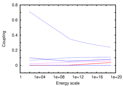
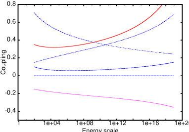
  Figure 1: Running of couplings for the first and second benchmark points in Type-II 2HDM. The line held steady at 0 is for $\lambda_{5}$ (dash-dot), the slowly falling line is for $Y^{t}_{2}$ (short dash-dot). The other four lines are, from top to bottom at the right-edge, (i) $\lambda_{3}$ (short dash), $\lambda_{2}$ (long dash), $\lambda_{4}$ (dot) and $\lambda_{1}$ (solid) for the left plot (BMtype2-1), (ii) $\lambda_{1}$ (solid), $\lambda_{3}$ (short dash), $\lambda_{2}$ (long dash) and $\lambda_{4}$ (dot) for the right plot (BMtype2-2).

• The second benchmark point (BMtype2-2) is specified by $\lambda_{1}=0.35$, $\lambda_{2}=0.10$, $\lambda_{3}=0.15$, $\lambda_{4}=-0.15$, and $\lambda_{5}=0$; $\tan\beta$ is constrained at $46.0$, and $m_{12}>10$ GeV. The Yukawa couplings are $Y_{1}^{b}=0.84$, $Y_{1}^{\tau}=0.33$, and $Y_{2}^{t}=0.71$. Note that all the couplings remain perturbative till the Planck scale for this benchmark.

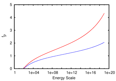
Figure 2: Variation of $f_{\rho_{1}}$ (red, solid) and $f_{\rho_{2}}$ (blue, dashed) with energy for Type-II 2HDM.

The Yukawa coupling $Y^{t}_{2}$ goes down with energy (see Fig. 1 or Eq. (LABEL:rge2)), while the scalar quartics either remain stable or increase. This destabilizes the VC for $\rho_{2}$. The destablization is more for higher values of the $\lambda_{i}$ couplings. We show, in Fig. 2, the behaviour of $f_{\rho_{1}}$ and $f_{\rho_{2}}$ for BMtype2-2; the former is more under control than the latter, as expected. While it may appear that the VCs are satisfied only at the electroweak scale but goes unmanageably out of control at higher $q^{2}$, we again stress that (i) this is only a one-loop calculation and unless the higher-order terms are computed, there is no way to know whether the behaviour is stable; and (ii) there may be some new physics at an intermediate scale that modifies the VCs. Also note that the fine-tuning of the physical scalar masses will be different, the corresponding functions $f_{h}$ and $f_{H}$ being some combinations of $f_{\rho_{1}}$ and $f_{\rho_{2}}$.

3.3 Flipped

The flipped 2HDM is very similar to Type-II, in fact, if we neglect the $\tau$ Yukawa coupling, they are identical. So we expect almost the same behaviour: a very tight constraint on $\lambda_{2}$, which turns out to be below $0.05$, and range for $\tan\beta$ is from 40.3 to 50.5. We take $m_{12}>10$ GeV to keep $m_{H^{+}}>300$ GeV. The Higgs mixing angle $\alpha$ lies between $-0.025$ and $-0.019$.

Our scan range is

$$0.1\leq\lambda_{1}\leq 0.4\,,\ \ 0\leq\lambda_{2}\leq 0.2\,,\ \ -0.05\leq\lambda_{3}\leq 0.2\,,\ \ -0.05\leq\lambda_{4}\leq 0.25\,,$$ (25)

and $\lambda_{5}=0$. The allowed range of $\tan\beta$ is $40.3<\tan\beta<50.5$.

• For the first benchmark (BMflip-1), we take $\lambda_{1}=0.35$, $\lambda_{2}=0.05$, $\lambda_{3}=0.18$, $\lambda_{4}=-0.045$, $\lambda_{5}=0$ and $\tan\beta=49.0$. The Yukawa couplings are, $Y_{1}^{b}=0.90$, $Y_{2}^{\tau}=0.007$, and $Y_{2}^{t}=0.71$. Note that all the couplings are well-behaved till the Planck scale.

  

  

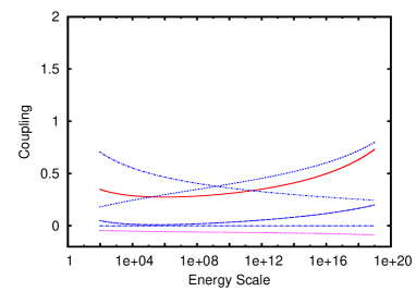
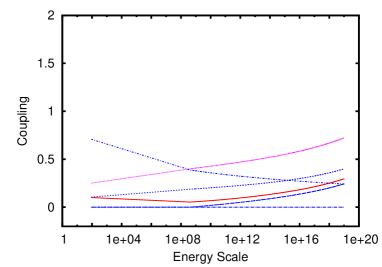
  Figure 3: Running of couplings for the first and second benchmark points in the flipped 2HDM. The line held steady at 0 is for $\lambda_{5}$ (dash-dot), the slowly falling line is for $Y^{t}_{2}$ (short dash-dot). Among the others, for BMflip-1 (left plot), lines at the left edge are for $\lambda_{1}$ (solid), $\lambda_{3}$ (short dash), $\lambda_{2}$ (long dash), and $\lambda_{4}$ (dot) (from top to bottom) respectively. For BMflip-2 (right plot), lines at the left edge, from top to bottom, are for $\lambda_{4}$ (dot), $\lambda_{3}$ (short dash), $\lambda_{1}$ (solid) and $\lambda_{2}$ (long dash) respectively.

• The second benchmark (BMflip-2) is taken at $\lambda_{1}=0.1$, $\lambda_{2}=0.0$, $\lambda_{3}=0.19$, $\lambda_{4}=0.07$, $\lambda_{5}=0.0$ and $\tan\beta=42.5$. The Yukawa couplings are, $Y_{1}^{b}=0.778$, $Y_{2}^{\tau}=0.007$, $Y_{2}^{t}=0.7075$. Again, the model is stable till the Planck scale.

The stability of $f_{\rho_{1}}$ and $f_{\rho_{2}}$ is shown in Fig. 4 for BMflip-1.

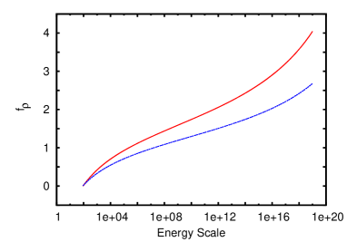
Figure 4: Variation of $f_{\rho_{1}}$ (red, solid) and $f_{\rho_{2}}$ (blue, dashed) with energy for flipped 2HDM.

3.4 Lepton specific

Lepton-specific 2HDM also needs large values of $\tan\beta$ because the $\tau$-Yukawa coupling has to play the deciding role in the VC of $\rho_{1}$. In fact, it is even larger than that needed for Type-II and flipped 2HDM, as $m_{\tau}<m_{b}$.

Our scan range is

$$0\leq\lambda_{1}\leq 0.4\,,\ \ 0.0\leq\lambda_{2}\leq 0.4\,,\ \ -0.05\leq\lambda_{3}\leq 0.4\,,\ \ -0.05\leq\lambda_{4}\leq 0.4\,.$$ (26)

We find $141<\tan\beta<221$ with $\lambda_{5}=0$, and $-0.008<\alpha<-0.004$. Such large values of $\tan\beta$ is known to be problematic for possible non-perturbative behavious of the Yukawa couplings. As the Yukawa couplings have a negative pull on the quartics, large values for them tend to make the quartic couplings negative very quickly, making the potential unstable. In fact, for the entire allowed parameter space, such instability occurs below 1 TeV. Thus, one is forced to predict some cutoff at 1 TeV or below, above which a new dynamics takes over.

4 Summary

We have discussed the fine-tuning problem in the context of 2HDMs. In particular, we try to find the parameter space in several 2HDMs where the quadratic divergences of the scalar masses are under control.

We have kept ourselves confined only among those models that do not have any tree-level FCNC, and explore the possible parameter space where the Veltman conditions are satisfied for all the scalars. This is helped by the fermionic couplings of the scalars; Type-I 2HDM does not possess this feature, $\Phi_{1}$ does not have any fermionic coupling, so a successful cancellation of the $\Lambda^{2}$ terms is never possible, even if we take some quartic scalar couplings to be negative. We emphasize that our results are valid only for standalone 2HDMs, not when they are embedded in a larger theory.

In contrast with the SM (or the Type-I 2HDM), it is possible to find a parameter space for all the other three 2HDMs where the VCs are satisfied. This may not seem very surprising, as we have more parameters to play with, but note that we also have a large number of constraints: the stability of the potential, the existence of a CP-even minimum, the lightest CP-even neutral scalar close to 125 GeV, the constraint on the charged Higgs mass, the necessity of making the 125 GeV scalar behave like the SM Higgs boson, etc. That such constraints are important can be seen from the lepton-specific 2HDM, where the requirement of large $\tan\beta$ forces large Yukawa couplings and destroys the stability of the potential at most above 1 TeV. However, it is too early to say that such models are not compatible with both LHC data and solution of the naturalness problem; 1 TeV is hardly a scale where one would talk about naturalness, and two-loop corrections might push the limit a bit upwards.

We find solutions only for the large $\tan\beta$ case: about 31.5 for Type-II, 42.5 for flipped, and about 140 for lepton-specific models. In fact, the allowed values of $\tan\beta$ are severely restricted. The dependence of $\tan\beta$ on $\lambda_{1}$ is almost linear for Type II and flipped 2HDM; for the lepton specific 2HDM the dependence is more complicated. Anyway, we believe that this is an interesting result in the study of 2HDM.

Not all the solutions for Type-II and flipped 2HDMs are valid till the Planck scale. In particular, whenever we start with a large quartic coupling, there is always a chance that the Landau pole will be hit before $M_{Pl}$. Fortunately, for most part of the parameter space, even if the blow-up occurs, the scale is rather large and beyond the reach of the LHC. Such a behaviour may be taken as indicative of some other new physics taking over at that scale. For lepton-specific models, the instability demands some new physics possibly within the LHC reach.

Everything would have been perfect if the VCs were absolutely stable with the scale variation. Unfortunately, this is not so. But this may be due to the simplistic approach of keeping only the one-loop terms; at higher-orders, we might expect a scale independence.

5 Acknowledgements

The authors thank Debtosh Chowdhury for pointing out a mistake in the first version of the paper. A.K. acknowledges DST, Government of India, and CSIR, Government of India, for research support. I.C. acknowledges CSIR, Govt. of India, for a research fellowship.

Appendix A RG equations

Without the Yukawa couplings, the one-loop RGEs are

$$16\pi^{2}\beta_{\lambda_{1}} = 6\lambda_{1}^{2}+2\lambda_{3}^{2}+\lambda_{4}^{2}+\lambda_{5}^{2}+2\lambda_{3}\lambda_{4}-\frac{3}{2}\lambda_{1}\left(g_{1}^{2}+3g_{2}^{2}\right)+\frac{3}{8}(g_{1}^{4}+2g_{1}^{2}g_{2}^{2}+3g_{2}^{4})\,,$$

$$16\pi^{2}\beta_{\lambda_{2}} = 6\lambda_{2}^{2}+2\lambda_{3}^{2}+\lambda_{4}^{2}+\lambda_{5}^{2}+2\lambda_{3}\lambda_{4}-\frac{3}{2}\lambda_{2}\left(g_{1}^{2}+3g_{2}^{2}\right)+\frac{3}{8}(g_{1}^{4}+2g_{1}^{2}g_{2}^{2}+3g_{2}^{4})\,,$$

$$16\pi^{2}\beta_{\lambda_{3}} = (\lambda_{1}+\lambda_{2})(3\lambda_{3}+\lambda_{4})+2\lambda_{3}^{2}+\lambda_{4}^{2}+\lambda_{5}^{2}+\frac{3}{8}\left(3g_{2}^{4}+g_{1}^{4}-2g_{1}^{2}g_{2}^{2}\right)-\frac{3}{2}\lambda_{3}\left(3g_{2}^{2}+g_{1}^{2}\right)\,,$$

$$16\pi^{2}\beta_{\lambda_{4}} = \left(\lambda_{1}+\lambda_{2}+4\lambda_{3}+2\lambda_{4}\right)\lambda_{4}+4\lambda_{5}^{2}+\frac{3}{2}g_{1}^{2}g_{2}^{2}-\frac{3}{2}\lambda_{4}\left(3g_{2}^{2}+g_{1}^{2}\right)\,,$$

$$16\pi^{2}\beta_{\lambda_{5}} = \left(\lambda_{1}+\lambda_{2}+4\lambda_{3}+6\lambda_{4}\right)\lambda_{5}-\frac{3}{2}\lambda_{5}\left(3g_{2}^{2}+g_{1}^{2}\right)\,.$$

Once we include the Yukawa couplings, which are model-specific, the RGEs turn out to be as follows.

• Type II:

  $$\left(16\pi^{2}\beta_{\lambda_{1}}\right)_{total} = 16\pi^{2}\beta_{\lambda_{1}}+6\lambda_{1}\left(Y_{1}^{b}\right)^{2}+2\lambda_{1}\left(Y_{1}^{\tau}\right)^{2}-6\left(Y_{1}^{b}\right)^{4}-2\left(Y_{1}^{\tau}\right)^{4}\,,$$

  $$\left(16\pi^{2}\beta_{\lambda_{2}}\right)_{total} = 16\pi^{2}\beta_{\lambda_{2}}+6\lambda_{2}\left(Y_{2}^{t}\right)^{2}-6\left(Y_{2}^{t}\right)^{4}\,,$$

  $$\left(16\pi^{2}\beta_{\lambda_{3}}\right)_{total} = 16\pi^{2}\beta_{\lambda_{3}}+6\lambda_{3}\left(Y_{1}^{b}\right)^{2}+2\lambda_{3}\left(Y_{1}^{\tau}\right)^{2}+3\lambda_{3}\left(Y_{2}^{t}\right)^{2}\,,$$

  $$\left(16\pi^{2}\beta_{\lambda_{4}}\right)_{total} = 16\pi^{2}\beta_{\lambda_{4}}+6\lambda_{4}\left(Y_{1}^{b}\right)^{2}+2\lambda_{4}\left(Y_{1}^{\tau}\right)^{2}+3\lambda_{4}\left(Y_{2}^{t}\right)^{2}\,,$$

  $$\left(16\pi^{2}\beta_{\lambda_{5}}\right)_{total} = 16\pi^{2}\beta_{\lambda_{5}}+6\lambda_{5}\left(Y_{1}^{b}\right)^{2}+2\lambda_{5}\left(Y_{1}^{\tau}\right)^{2}+3\lambda_{5}\left(Y_{2}^{t}\right)^{2}\,.$$

• Lepton specific:

  $$\left(16\pi^{2}\beta_{\lambda_{1}}\right)_{total} = 16\pi^{2}\beta_{\lambda_{1}}+2\lambda_{1}\left(Y_{1}^{\tau}\right)^{2}-2\left(Y_{1}^{\tau}\right)^{4}\,,$$

  $$\left(16\pi^{2}\beta_{\lambda_{2}}\right)_{total} = 16\pi^{2}\beta_{\lambda_{2}}+6\lambda_{2}\left(Y_{2}^{t}\right)^{2}+6\lambda_{2}\left(Y_{2}^{b}\right)^{2}-6\left(Y_{2}^{t}\right)^{4}-6\left(Y_{2}^{b}\right)^{4}\,,$$

  $$\left(16\pi^{2}\beta_{\lambda_{3}}\right)_{total} = 16\pi^{2}\beta_{\lambda_{3}}+6\lambda_{3}\left(Y_{2}^{b}\right)^{2}+2\lambda_{3}\left(Y_{1}^{\tau}\right)^{2}+3\lambda_{3}\left(Y_{2}^{t}\right)^{2}\,,$$

  $$\left(16\pi^{2}\beta_{\lambda_{4}}\right)_{total} = 16\pi^{2}\beta_{\lambda_{4}}+6\lambda_{4}\left(Y_{2}^{b}\right)^{2}+2\lambda_{4}\left(Y_{1}^{\tau}\right)^{2}+3\lambda_{4}\left(Y_{2}^{t}\right)^{2}\,,$$

  $$\left(16\pi^{2}\beta_{\lambda_{5}}\right)_{total} = 16\pi^{2}\beta_{\lambda_{5}}+6\lambda_{5}\left(Y_{2}^{b}\right)^{2}+2\lambda_{5}\left(Y_{1}^{\tau}\right)^{2}+3\lambda_{5}\left(Y_{2}^{t}\right)^{2}\,.$$

• Flipped:

  $$\left(16\pi^{2}\beta_{\lambda_{1}}\right)_{total} = 16\pi^{2}\beta_{\lambda_{1}}+6\lambda_{1}\left(Y_{1}^{b}\right)^{2}-6\left(Y_{1}^{b}\right)^{4}\,,$$

  $$\left(16\pi^{2}\beta_{\lambda_{2}}\right)_{total} = 16\pi^{2}\beta_{\lambda_{2}}+6\lambda_{2}\left(Y_{2}^{t}\right)^{2}+2\lambda_{2}\left(Y_{2}^{\tau}\right)^{2}-6\left(Y_{2}^{t}\right)^{4}-2\left(Y_{2}^{\tau}\right)^{4}\,,$$

  $$\left(16\pi^{2}\beta_{\lambda_{3}}\right)_{total} = 16\pi^{2}\beta_{\lambda_{3}}+3\lambda_{3}\left(Y_{2}^{t}\right)^{2}+2\lambda_{3}\left(Y_{2}^{\tau}\right)^{2}+6\lambda_{3}\left(Y_{1}^{b}\right)^{2}\,,$$

  $$\left(16\pi^{2}\beta_{\lambda_{4}}\right)_{total} = 16\pi^{2}\beta_{\lambda_{4}}+3\lambda_{4}\left(Y_{2}^{t}\right)^{2}+2\lambda_{4}\left(Y_{2}^{\tau}\right)^{2}+6\lambda_{4}\left(Y_{1}^{b}\right)^{2}\,,$$

  $$\left(16\pi^{2}\beta_{\lambda_{5}}\right)_{total} = 16\pi^{2}\beta_{\lambda_{5}}+3\lambda_{5}\left(Y_{2}^{t}\right)^{2}+2\lambda_{5}\left(Y_{2}^{\tau}\right)^{2}+6\lambda_{5}\left(Y_{1}^{b}\right)^{2}\,.$$

Note that we have not talked about the RGEs of Type-I 2HDM, the reasons are given in the main body of the paper.

The Yukawa RGEs are:

• Type-II:

  $$16\pi^{2}\beta_{Y_{1}^{b}} = \frac{1}{2}Y_{1}^{b}\left[-8g_{s}^{2}-\frac{9}{4}g_{2}^{2}-\frac{5}{12}g_{1}^{2}+\frac{9}{2}\left(Y_{1}^{b}\right)^{2}+\left(Y_{1}^{\tau}\right)^{2}+\frac{1}{2}\left(Y_{2}^{t}\right)^{2}\right]\,$$

  $$16\pi^{2}\beta_{Y_{2}^{t}} = \frac{1}{2}Y_{2}^{t}\left[-8g_{s}^{2}-\frac{9}{4}g_{2}^{2}-\frac{17}{12}g_{1}^{2}+\frac{9}{2}\left(Y_{2}^{t}\right)^{2}+\frac{1}{2}\left(Y_{1}^{b}\right)^{2}\right]\,$$

  $$16\pi^{2}\beta_{Y_{1}^{\tau}} = \frac{1}{2}Y_{1}^{\tau}\left[-\frac{9}{4}g_{2}^{2}-\frac{15}{4}g_{1}^{2}+3\left(Y_{1}^{b}\right)^{2}+\frac{5}{2}\left(Y_{1}^{\tau}\right)^{2}\right]\,$$

• Lepton specific:

  $$16\pi^{2}\beta_{Y_{2}^{b}} = \frac{1}{2}Y_{2}^{b}\left[-8g_{s}^{2}-\frac{9}{4}g_{2}^{2}-\frac{5}{12}g_{1}^{2}+\frac{9}{2}\left(Y_{2}^{b}\right)^{2}+\frac{3}{2}\left(Y_{2}^{t}\right)^{2}\right]\,$$

  $$16\pi^{2}\beta_{Y_{2}^{t}} = \frac{1}{2}Y_{2}^{t}\left[-8g_{s}^{2}-\frac{9}{4}g_{2}^{2}-\frac{17}{12}g_{1}^{2}+\frac{9}{2}\left(Y_{2}^{t}\right)^{2}+\frac{3}{2}\left(Y_{2}^{b}\right)^{2}\right]\,$$

  $$16\pi^{2}\beta_{Y_{1}^{\tau}} = \frac{1}{2}Y_{1}^{\tau}\left[-\frac{9}{4}g_{2}^{2}-\frac{15}{4}g_{1}^{2}+\frac{5}{2}\left(Y_{1}^{\tau}\right)^{2}\right]\,$$

• Flipped:

  $$16\pi^{2}\beta_{Y_{1}^{b}} = \frac{1}{2}Y_{1}^{b}\left[-8g_{s}^{2}-\frac{9}{4}g_{2}^{2}-\frac{5}{12}g_{1}^{2}+\frac{9}{2}\left(Y_{1}^{b}\right)^{2}+\frac{1}{2}\left(Y_{2}^{t}\right)^{2}\right]\,$$

  $$16\pi^{2}\beta_{Y_{2}^{t}} = \frac{1}{2}Y_{2}^{t}\left[-8g_{s}^{2}-\frac{9}{4}g_{2}^{2}-\frac{17}{12}g_{1}^{2}+\frac{9}{2}\left(Y_{2}^{t}\right)^{2}+\frac{1}{2}\left(Y_{1}^{b}\right)^{2}+\left(Y_{2}^{\tau}\right)^{2}\right]\,$$

  $$16\pi^{2}\beta_{Y_{2}^{\tau}} = \frac{1}{2}Y_{2}^{\tau}\left[-\frac{9}{4}g_{2}^{2}-\frac{15}{4}g_{1}^{2}+\frac{5}{2}\left(Y_{2}^{\tau}\right)^{2}+3\left(Y_{2}^{t}\right)^{2}\right]\,$$

Here $g_{s}$, $g_{1}$ and $g_{2}$ are gauge coupling constants of ${SU(3)}_{c}$ , $U(1)_{Y}$ and $SU(2)_{L}$ respectively, $\beta_{h}\equiv dh/dt$, and $t\equiv\ln(q^{2}/\mu^{2})$. Note that our definition of $t$ differs by a factor of 2 from that used by some authors.

A more compact form of the one-loop RGEs for the Yukawa couplings, valid for all 2HDMS, is [1]

$$16\pi^{2}\beta_{Y_{j}^{b}} = \frac{1}{2}a_{b}Y_{j}^{b}+\frac{1}{2}\sum_{k=1}^{n_{H}}T_{jk}Y_{k}^{b}$$ (A.8)

$$+\frac{1}{2}\sum_{k=1}^{n_{H}}\left(-2Y_{k}^{t}{Y_{j}^{t}}^{{\dagger}}Y_{k}^{b}+\frac{1}{2}Y_{k}^{t}{Y_{k}^{t}}^{{\dagger}}Y_{j}^{b}+Y_{j}^{b}{Y_{k}^{b}}^{{\dagger}}Y_{k}^{b}+\frac{1}{2}Y_{k}^{b}{Y_{k}^{b}}^{{\dagger}}Y_{j}^{b}\right)\,,$$

$$16\pi^{2}\beta_{Y_{j}^{t}} = \frac{1}{2}a_{t}Y_{j}^{t}+\frac{1}{2}\sum_{k=1}^{n_{H}}T_{jk}^{*}Y_{k}^{t}$$ (A.9)

$$+\frac{1}{2}\sum_{k=1}^{n_{H}}\left(-2Y_{k}^{b}{Y_{j}^{b}}^{{\dagger}}Y_{k}^{t}+\frac{1}{2}Y_{k}^{b}{Y_{k}^{b}}^{{\dagger}}Y_{j}^{t}+Y_{j}^{t}{Y_{k}^{t}}^{{\dagger}}Y_{k}^{t}+\frac{1}{2}Y_{k}^{t}{Y_{k}^{t}}^{{\dagger}}Y_{j}^{t}\right)\,,$$

$$16\pi^{2}\beta_{Y_{j}^{\tau}}=\frac{1}{2}a_{\tau}Y_{j}^{\tau}+\frac{1}{2}\sum_{k=1}^{n_{H}}T_{jk}Y_{k}^{\tau}+\frac{1}{2}\sum_{k=1}^{n_{H}}\left(\frac{1}{2}Y_{k}^{\tau}{Y_{k}^{\tau}}^{{\dagger}}Y_{j}^{\tau}+Y_{j}^{\tau}{Y_{k}^{\tau}}^{{\dagger}}Y_{k}^{\tau}\right)\,,$$ (A.10)

where

$$a_{b} = -8g_{s}^{2}-\frac{9}{4}g_{2}^{2}-\frac{5}{12}g_{1}^{2}\,,$$

$$a_{t} = -8g_{s}^{2}-\frac{9}{4}g_{2}^{2}-\frac{17}{12}g_{1}^{2}\,,$$

$$a_{\tau} = -\frac{9}{4}g_{2}^{2}-\frac{15}{4}g_{1}^{2}\,,$$

$$T_{jk} = 3tr\left(Y_{j}^{b}{Y_{k}^{b}}^{{\dagger}}+{Y_{j}^{t}}^{{\dagger}}Y_{k}^{t}\right)+tr\left(Y_{j}^{\tau}{Y_{k}^{\tau}}^{{\dagger}}\right)\,.$$ (A.11)

References

- [1] G. C. Branco, P. M. Ferreira, L. Lavoura, M. N. Rebelo, M. Sher and J. P. Silva, Phys. Rept. 516, 1 (2012) [arXiv:1106.0034 [hep-ph]].
- [2] S. L. Glashow and S. Weinberg, Phys. Rev. D 15, 1958 (1977).
- [3] E. A. Paschos, Phys. Rev. D 15, 1966 (1977).
- [4] G. C. Branco, W. Grimus and L. Lavoura, Phys. Lett. B 380, 119 (1996) [hep-ph/9601383].
- [5] F. J. Botella, G. C. Branco, A. Carmona, M. Nebot, L. Pedro and M. N. Rebelo, arXiv:1401.6147 [hep-ph].
- [6] G. Bhattacharyya, D. Das, and A. Kundu, arXiv:1402.0364.
- [7] M. J. G. Veltman, Acta Phys. Polon. B 12, 437 (1981).
- [8] M. B. Einhorn and D. R. T. Jones, Phys. Rev. D 46, 5206 (1992).
- [9] A. Kundu and S. Raychaudhuri, Phys. Rev. D 53, 4042 (1996) [hep-ph/9410291].
-
[10]
B. Grzadkowski and J. Wudka,
Phys. Rev. Lett. 103, 091802 (2009)
[arXiv:0902.0628 [hep-ph]];
A. Drozd, B. Grzadkowski and J. Wudka, JHEP 1204, 006 (2012) [arXiv:1112.2582 [hep-ph]]. - [11] I. Chakraborty and A. Kundu, Phys. Rev. D 87, 055015 (2013) [arXiv:1212.0394 [hep-ph]].
- [12] F. Bazzocchi and M. Fabbrichesi, Phys. Rev. D 87, no. 3, 036001 (2013) [arXiv:1212.5065 [hep-ph]].
- [13] I. Chakraborty and A. Kundu, Phys. Rev. D 89, 095032 (2014) [arXiv:1404.1723 [hep-ph]].
-
[14]
E. Ma,
Int. J. Mod. Phys. A 16, 3099 (2001)
[hep-ph/0101355];
R. Jora, S. Nasri and J. Schechter, Int. J. Mod. Phys. A 28, 1350036 (2013) [arXiv:1302.6344 [hep-ph]]. - [15] B. Grzadkowski and P. Osland, Phys. Rev. D 82, 125026 (2010) [arXiv:0910.4068 [hep-ph]].
- [16] W. Grimus, L. Lavoura, O. M. Ogreid and P. Osland, J. Phys. G 35, 075001 (2008) [arXiv:0711.4022 [hep-ph]]; Nucl. Phys. B 801, 81 (2008) [arXiv:0802.4353 [hep-ph]].
- [17] P. M. Ferreira, R. Santos and A. Barroso, Phys. Lett. B 603, 219 (2004) [Erratum-ibid. B 629, 114 (2005)] [hep-ph/0406231].
- [18] I. P. Ivanov, Phys. Rev. D 77, 015017 (2008) [arXiv:0710.3490 [hep-ph]].
- [19] A. Barroso, P. M. Ferreira, I. P. Ivanov and R. Santos, JHEP 1306, 045 (2013) [arXiv:1303.5098 [hep-ph]].
-
[20]
H. E. Haber and R. Hempfling,
Phys. Rev. D 48, 4280 (1993)
[hep-ph/9307201];
P. M. Ferreira, L. Lavoura and J. P. Silva, Phys. Lett. B 688, 341 (2010) [arXiv:1001.2561 [hep-ph]]. -
[21]
F. Mahmoudi and O. Stal,
Phys. Rev. D 81, 035016 (2010)
[arXiv:0907.1791 [hep-ph]];
O. Deschamps, S. Descotes-Genon, S. Monteil, V. Niess, S. T’Jampens and V. Tisserand, Phys. Rev. D 82, 073012 (2010) [arXiv:0907.5135 [hep-ph]];
X. -D. Cheng, Y. -D. Yang and X. -B. Yuan, arXiv:1401.6657 [hep-ph].