A $\kappa$-deformed Model of Growing Complex Networks with Fitness

Abstract

The Barabási-Bianconi (BB) fitness model can be solved by a mapping between the original network growth model to an idealized bosonic gas. The well-known transition to Bose-Einstein condensation in the latter then corresponds to the emergence of “super-hubs” in the network model. Motivated by the preservation of the scale-free property, thermodynamic stability and self-duality, we generalize the original extensive mapping of the BB fitness model by using the nonextensive Kaniadakis $\kappa$-distribution. Through numerical simulation and mean-field calculations we show that deviations from extensivity do not compromise qualitative features of the phase transition. Analysis of the critical temperature yields a monotonically decreasing dependence on the nonextensive parameter $\kappa$.

Keywords: complex networks, Bose-Einstein condensation, growing networks, nonextensive statistics.

Introduction

Over the last twenty years, research about complex networks has yielded many insights into a large number of real-world systems in various contexts, with systems as diverse as the World Wide Web, social media, power grids, transportation networks and gene regulation networks being prime examples, cf. [1, 2, 3] for reviews on the field. The network paradigm has proven very useful in quantifying the topology of interactions in these systems. In recent years the interest of the scientific community has shifted from analysis of purely static structures towards attempts at gaining insights into dynamically evolving or optimized networks [2]. In many applications statistical physics has provided a powerful toolbox, sometimes discovering surprising parallels between networked systems and other physical systems. One example of such a parallel is the Barabási-Bianconi (BB) model [4, 5], which describes a process of network evolution guided by a combination of preferential attachment and intrinsic fitness properties of nodes [2].

In [5], a mapping between the growing network and a bosonic gas undergoing a Bose-Einstein condensation was proposed, realized by means of extensive statistical mechanics, and solved via a mean field approach. No interactions between particles or energy level transitions were contemplated. Interesting behaviour is found when introducing a fictitious temperature parameter $T$ regulating the network dynamics. Even for $T\rightarrow 0$ the bosonic gas counterpart exhibits a ground state in which only half of the particles reach the minimum energy level, the others being scattered in fixed positions throughout the whole energy spectrum [5, 6]. This anomalous thermodynamic behavior is incompatible with the Boltzmann weight used for the original mapping. In fact, a purely physical perspective would suggest that in equilibrium all the bosons of the Bose-Einstein condensate populate the minimum energy level in the ground state. This anomaly has motivated research into applications of deformed non-Gaussian statistics [7, 8] and it is of interest to generalize the mapping between bosonic gases and growing networks by recurring to a nonextensive deformation of the original equilibrium Boltzmann-Gibbs distribution. Even though Information Theory seems to suggest a link between non-ergodic behavior and nonextensive statistics in nature, the emergence of non-Gaussian statistics for complex systems, as, e.g., growing complex networks, has not yet been fully understood [9].

To the best of our knowledge one recent study [10] of the BB model using Tsallis’ $q$-statistics [7] is the only previous investigation of extensions of the BB model to nonextensive statistics. Properties of the $q$-statistics make it very difficult to find exact results and the insights gained by [10] are limited to numerical simulation. Further, it has been argued [11] that non-extensive statistics should have the following characteristics: (i) preservation of scale-free property, (ii) self-duality, and (iii) thermodynamic stability. Even though the Tsallis $q$-exponential gives rise to power-laws in many real world modelling applications [7] it does not satisfy self-duality. This gives an added interest to the Kanidakis $\kappa$-distribution which meets all three requirements. The $\kappa$-deformed statistical mechanics was originally proposed in the context of non-linear kinetics in particle systems and is deeply linked to the structure of special relativity [11]. In the last decade, $\kappa$-deformed statistics have been successfully applied to model the distribution of stellar rotational velocities of dwarf stars [12], cosmic ray fluxes [11], the formation of Quark-Gluon plasmas [13], and the income distribution of the USA, UK, Germany and Italy [8]. Moreover, the use of $\kappa$-deformed statistics has led to some insight [14] in addressing the inadequacy of the Bose-Einstein distribution in predicting the fluid-superfluid transition temperature in ${}^{4}He$ . The latter gives an additional motivation for our application of $\kappa$-deformed statistics to models of network formation.

In this article we show that the Kaniadakis $\kappa$-distribution can be used to generalize the BB bosonic mapping. In contrast to previous numerical results based on $q$-statistics [10], analytical mean-field results can be retrieved with the $\kappa$-deformed distribution. Our findings show that the use of the Kaniadakis $\kappa$-distribution does not alter the qualitative presence of condensation. We show both analytically and numerically that the main influence of the nonextensive parameter is a systematic shift of the critical temperature with $\kappa$.

Our paper is organized as follows. In Section I we briefly review some of the properties of the BB fitness model and its original extensive mapping to a Bose-Einstein condensate. In Section II we summarize some basic results of the Kaniadakis $\kappa$-distribution and generalize them to the nonextensive mapping. Finally, in Section III numerical results for the critical temperatures for different values of the nonextensive parameter are presented and compared to analytical findings. In the same section, we will also analyze the degree distribution of our generalized model, by using both analytical and numerical methods.

1 The Barabási-Bianconi Fitness Model

The BB model [5, 4] is a model that describes network evolution as an incremental growth process. At each time step a new node, say $j$, is added to the growing network and it is assigned a fitness $\eta_{j}$, i.e. a positive real number randomly drawn from a distribution $\rho\left(\eta\right)$. Then connections from $j$ to $m$ of the $n$ old nodes are formed one at a time, such that each time old nodes can attract a link from the new node with a probability given by

$$\Pi\left(k_{i},\eta_{i}\right)=\frac{\eta_{i}k_{i}}{\overset{n}{\underset{j=1}{\sum}}\eta_{j}k_{j}},$$ (1.1)

which is proportional to both the fitness $\eta_{i}$ and the degree $k_{i}$ of the node. This preferential attachment dynamics consistently reproduces some features present in many real world networks [2, 1], which exhibit big hubs with different age. The fitness parameter influences the competition for new connections. Without it, as in the “pure” preferential attachement model [15], “older” nodes are always on average more connected than younger nodes. Including the fitness aspects, highly connected nodes can be old nodes, but could also be “young” nodes with high intrinsic fitness. One of the most interesting features of the Barabási-Albert (BA) and BB models is the fact that they both can produce scale-free networks with power-law degree distributions $P\left(k\right)$ [5, 4], namely $P\left(k\right)\sim Ax^{-\gamma}$ for $x\rightarrow+\infty$, with scaling exponents $\gamma$ typically between 2 and 3 and compatible with those of many natural and human systems [2, 1].

1.1 Extensive mapping with a Bose-Einstein system and the Network Condensation

In [5], Bianconi realized a mapping between the asymptotic structure of the network and an hypothetical Bose gas by setting $\eta_{i}=e^{-\beta\epsilon_{i}}$. In this formulation $\beta$ is the inverse of a fictitious network temperature $T$ and $\epsilon_{i}$ is the energy level for node $i$. Every node of the network represents one energy level while every edge between two nodes $i$ and $j$ represents two non-interacting particles, one on level $\epsilon_{i}$ and the other on level $\epsilon_{j}$. It can be shown [5, 4, 6, 16] that preferential attachment driven by the probability $\Pi$ undergoes a phase transition at some critical temperature $T_{c}$, which is formally identical to that of Bose-Einstein condensation. At high temperatures, $T>T_{c}$, even in the thermodynamic limit the hubs of the network participate in a competition for the “survival-of-the-fittest” while at lower temperatures, for $T<T_{c}$, a unique “super-hub” eventually emerges and wins the competition [16] (this represents a “winner-takes-all” phenomenon encountered in many real-world applications [2]). By using the network mapping of edges to a physical system of $2N$ bosons, it is evident that eventually only half of them can “reach” the fundamental energy level of the network, which corresponds to the highest fitness present.

2 Kaniadakis Mapping

The Kaniadakis $\kappa$-distribution [11], was originally introduced in 2002 and later re-obtained within the framework of a Jaynes Maximum Entropy principle [17], which starts from a generalized system entropy $S_{\kappa}$ given by

$$S_{\kappa}=-\underset{l}{\sum}p_{l}\ln_{\kappa}\,p_{l}=-\underset{l}{\sum}p_{l}\frac{\left(p_{l}\right)^{\kappa}-\left(p_{l}\right)^{-\kappa}}{2\kappa}$$ (2.1)

with $p_{l}$ being the probability of the system being in state $l$ and $\kappa\in\left(-1,1\right)$. It can be shown that the generalized logarithm $\ln_{\kappa}\left(x\right)$ is self-scaling and self-dual [17], as the ordinary logarithm $\ln\left(x\right)$ of the Boltzmann-Shannon entropy $S=-\sum p_{l}\ln\left(p_{l}\right)$.

The parameter $\kappa$ can be seen as a deviation from extensivity, as $\ln_{\kappa}\left(x\right)$ recovers the extensive case when $\kappa\rightarrow 0$. The inverse of the generalized logarithm is the generalized exponential [11, 17],

$$e_{\kappa}^{x}=\left(\kappa x+\sqrt{1+\kappa^{2}x^{2}}\right)^{\frac{1}{\kappa}}$$ (2.2)

which has power-law tails given by the asymptotics $e_{\kappa}^{x}\sim 2\left|\kappa x\right|^{\frac{\pm 1}{\left|\kappa\right|}}$ for $x\rightarrow\pm\infty$ [17]. It has been shown [11] that this $\kappa$-deformed exponential is a positive monotonically increasing function which is symmetric with respect to the nonextensive parameter $\kappa$ ($e_{\kappa}^{x}=e_{-\kappa}^{x}$) and satisfies $\forall x\in\mathbb{R},\;e_{\kappa}^{x}e_{\kappa}^{-x}=1$ and $\forall x,a\in\mathbb{R},\;e_{\kappa}^{ax}=\left(e_{a\kappa}^{x}\right)^{a}$.

Mimicking the mapping of the original BA model, we consider the fitness $\eta_{i}$ as

$$\eta_{i}=e_{\kappa}^{-\beta\epsilon_{i}}=\left[\kappa\left(-\beta\epsilon_{i}\right)+\sqrt{1+\kappa^{2}\beta^{2}\epsilon_{i}^{2}}^{\frac{1}{\kappa}}\right]$$ (2.3)

where the energy level $\epsilon_{i}=-\beta^{-1}\ln_{\kappa}\eta_{i}$ can be thought of as a transformation of a random variable distributed according to the distribution $g\left(\epsilon\right)$, the latter having the physical interpretation of an energy level density. In order for the network to undergo a Bose-Einstein phase transition, it is required that $g\left(\epsilon\right)\rightarrow 0$ when $\epsilon\rightarrow 0$ [5, 4, 10]. With this generalization, Eq. (1.1) for the degree $k_{i}$ becomes

$$\frac{dk_{i}}{dt}=m\frac{e_{\kappa}^{-\beta\epsilon_{i}}k_{i}\left(\epsilon_{i},t_{i},t\right)}{\underset{j}{\sum}e_{\kappa}^{-\beta\epsilon_{j}}k_{j}\left(\epsilon_{j},t_{j},t\right)}=m\frac{e_{\kappa}^{-\beta\epsilon_{i}}k_{i}\left(\epsilon_{i},t_{i},t\right)}{Z_{\kappa}\left(t\right)}$$ (2.4)

where $Z_{\kappa}$ is our network partition function. We want to look for solutions $k_{i}$ which mimic the analytical form of the solution for the BA model [5],

$$k_{i}\left(\epsilon_{i},t_{i},t\right)=A_{m}\left(\frac{t}{t_{i}}\right)^{f_{\kappa}\left(\epsilon_{i}\right)}$$ (2.5)

where $A_{m}$ depends on the parameter $m$ while $f_{\kappa}=f_{\kappa}\left(\epsilon_{i}\right)$ is some still unknown dynamic exponent strictly bounded by 0 and 1. This functional form implies that the number of connections of every node increases in time ($f_{\kappa}>0$) but not as fast or faster than $t$ itself ($f_{\kappa}<1$). We can solve the above differential equation by applying a mean field approximation, in which we replace the partition sum $Z_{\kappa}$ by its average $\left\langle Z_{\kappa}\right\rangle$,

$$\left\langle Z_{\kappa}\right\rangle=A_{m}\int d\epsilon g\left(\epsilon\right)\frac{e_{\kappa}^{-\beta\epsilon}}{1-f_{\kappa}\left(\epsilon\right)}\left(t-t^{f_{\kappa}\left(\epsilon\right)}\right)\;.$$ (2.6)

For this purpose we introduce a chemical potential $\mu$ and a mean fugacity $z_{\kappa}=e_{\kappa}^{\beta\mu}$ and hence by using the thermodynamical stability of the deformed $\kappa$-exponential [17] one obtains:

$$\left\langle Z_{\kappa}\right\rangle\sim A_{m}\frac{t}{z_{\kappa}}+O\left(t^{\alpha}\right)\;.$$ (2.7)

Here $\alpha=f_{\kappa}\left(\epsilon\right)-1<0$ and then $t^{\alpha}\rightarrow 0$ in the thermodynamic limit. Comparing to the extensive case (obtained when $\kappa\rightarrow 0$), it has to be $\left\langle Z_{\kappa}\right\rangle\overset{\kappa\rightarrow 0}{\longrightarrow}mt/z$ for big enough networks. As by construction $A_{m}$ is independent of $\kappa$ we can choose $A_{m}=m$. Within this approximation Eq. (2.4) has a solution of the same form as given in Eq. (2.5) with a dynamic exponent $f_{\kappa}\left(\epsilon_{i}\right)=e_{\kappa}^{\beta\mu_{\kappa}}e_{\kappa}^{-\beta\epsilon_{i}}$. As $f_{\kappa}\left(\epsilon_{i}\right)\overset{\kappa\rightarrow 0}{\longrightarrow}e^{-\beta\left(\epsilon_{i}-\mu\right)}$ these results recover what is already known in the extensive limit [5].

By the definition of $z_{k}$ and exploiting the self-duality of the $\kappa$-exponential [17], we have that

$$I_{\beta}\left(\mu_{\kappa}\right)=\int d\epsilon g\left(\epsilon\right)\frac{1}{e_{\kappa}^{-\beta\mu_{\kappa}}e_{\kappa}^{\beta\epsilon}-1}=1\>.$$ (2.8)

In the integrand of this integral we can recognize the distribution $n_{\kappa}\left(\epsilon\right)$,

$$n_{\kappa}\left(\epsilon\right)=\frac{1}{e_{\kappa}^{-\beta\mu_{\kappa}}e_{\kappa}^{\beta\epsilon}-1}\underset{\kappa\rightarrow 0}{\longrightarrow}n\left(\epsilon\right)=\frac{1}{e^{\beta\left(\epsilon-\mu\right)}-1}$$ (2.9)

which, in our context, represents a deformed Bose-Einstein distribution, with the very same properties of monotonicity as the original Bose-Einstein distribution $n\left(\epsilon\right)$ in the non-extensive case.

Contrary to the case of the fitness model generalized with the Tsallis entropy [10], the Bose-Einstein distribution $n_{\kappa}\left(\epsilon\right)$ can be rewritten in a more insightful way by using properties of the $\kappa$-deformed exponential [11, 17]. In fact, by using $e_{\kappa}^{x}=\exp\left(\frac{1}{\kappa}\text{arcsinh}\,\kappa x\right)$, one can define a $\kappa$-deformed sum $\overset{\kappa}{\oplus}$ [11], such that $\left(\mathbb{R},\overset{\kappa}{\oplus}\right)$ is an Abelian group and

$$e_{\kappa}^{x}e_{\kappa}^{y}=e_{\kappa}^{\left(x\overset{\kappa}{\oplus}y\right)}=\exp\left(x\sqrt{1+\kappa^{2}y^{2}}+y\sqrt{1+\kappa^{2}x^{2}}\right)\;.$$ (2.10)

This recovers the usual property of exponentials in the extensive limit, i.e. $e_{\kappa}^{x}e_{\kappa}^{y}\overset{\kappa\rightarrow 0}{\longrightarrow}e^{x+y}$. From a physical point of view, it has to be remarked that this $\kappa$-deformed sum emerges naturally from the composition law of relativistic momenta in the framework of special relativity [11]. It is straightforward to generalize these formulas to a $\kappa$-deformed subtraction $\overset{\kappa}{\ominus}$ such that, $x\overset{\kappa}{\ominus}y=x\overset{\kappa}{\oplus}(-y)$ and

$$n_{\kappa}\left(\epsilon\right)=\frac{1}{e_{\kappa}^{\beta\left(\epsilon\overset{\kappa}{\ominus}\mu\right)}-1}$$ (2.11)

is formally equivalent to a Bose-Einstein-like distribution for a system whose energy levels are distributed according to a certain density $g\left(\epsilon\right)$. Here, however, the differences between the single particle energy and the chemical potential of the whole ensemble have to be interpreted in a $\kappa$-deformed way.

Exactly as in the original Bose-Einstein distribution, because of the physical meaning of $n_{\kappa}\left(\epsilon\right)$ as the probability of having a particle with energy between $\epsilon$ and $\epsilon+d\epsilon$, it has to be

$$n_{\kappa}\left(\epsilon\right)\geq 0\rightarrow\epsilon\overset{\kappa}{\ominus}\mu\geq 0\rightarrow\frac{\epsilon}{\sqrt{1+\kappa^{2}\epsilon^{2}}}\geq\frac{\mu}{\sqrt{1+\kappa^{2}\mu^{2}}}$$ (2.12)

which, as in the extensive case, implies that $\mu\leq\epsilon_{min}=0$ for bosonic systems.

Similar to the originally proposed model in this generalized BB model a Bose-Einstein phase transition occurs as long as $g\left(\epsilon\right)\rightarrow 0$ for $\epsilon\rightarrow 0$, i.e. if

$$I_{\beta}\left(\mu=0\right)=\int d\epsilon g\left(\epsilon\right)n_{\kappa}\left(\epsilon\right)<1\;.$$ (2.13)

We will present analytical and numerical estimates for the critical temperature in the next section.

3 Generalized Barabási-Bianconi Model: Numerical and Analytical Computations

3.1 Critical Temperature and Nonextensivity Parameter

Following arguments of [5] it can be seen that the Bose-Einstein condensation on the network corresponds to an almost zero value for the chemical potential $\mu$, which can be computed using a preliminary result we obtained while solving Eq. (2.4), i.e.

$$\mu\sim-\frac{1}{\beta}\text{ln}_{\kappa}\left(\frac{\left\langle Z_{\kappa}\right\rangle}{mt}\right)$$

where the $\kappa$-deformed logarithm was defined as in Eq. (2.1) and where the last approximation was made in order to solve Eq. (2.4). Estimates for the average partition function $\left\langle Z_{\kappa}\right\rangle$ over an ensembles of moderately sized networks can be obtained numerically.

We choose a simple distribution for $g\left(\epsilon\right)$ which is compatible with the occurrence of condensation and which also allows for easy comparisons with the numerical results of [5, 6], i.e. we use $g\left(\epsilon\right)=2\epsilon$ with corresponding energies $\epsilon\in(0,1)$. To obtain the phase diagram $\left|\mu\right|$ vs $T$ we carried out numerical simulations for varying network size $N$. As stated in [5], and confirmed in [10], for temperatures higher than the critical temperature $T_{c}^{\left(\kappa\right)}$ (in which $\mu$ vanishes) the network is in the fit-get-rich (FGR) phase, while under $T_{c}^{\left(\kappa\right)}$ one or more giant hubs appear and the nodes “condensate” their links to them, the whole network being in the winner-takes-all phase.

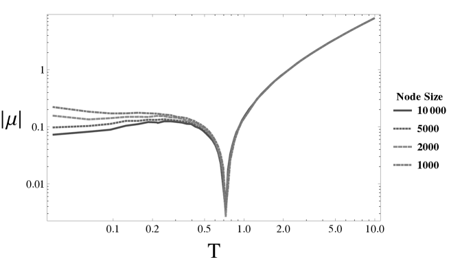
Figure 3.1: Phase diagram for different size ensembles of the generalized BB network, with $N=\{10^{3},2\cdot 10^{3},5\cdot 10^{3},10^{4}\}$ nodes and respectively averaged over $\{800,400,200,120\}$ different configurations, all with $m=2$ and $\kappa=0.9$. The critical temperature $T_{c}^{\left(0.9\right)}\simeq 0.76$ is statistically lower than the one reported in the extensive case [5], for $\kappa=0$, $T_{c}\simeq 0.8$. A scaling phenomenon is evident, following the decrease in temperature.

By averaging over 800 network realizations we determined a critical temperature $T_{c}^{\left(0.9\right)}=0.732\pm 0.002$ for a network ensemble with $m=2$, $\kappa=0.9$ and $N=1000$. This temperature is considerably lower than the one observed in the extensive ($\kappa=0$) case, in which $T_{c}^{\left(0\right)}=0.792\pm 0.002$, a value compatible with the previous finding of $T_{c}^{+}=0.8\pm 0.1$ in [5], and in [10].

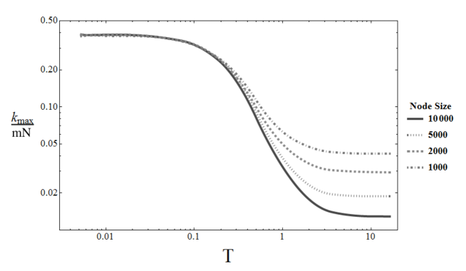
Figure 3.2: Average fraction of connections for the biggest hub, $k_{max}/mt$, inside a generalized BB network of $N=\{10^{3},2\cdot 10^{3},5\cdot 10^{3},10^{4}\}$ nodes, respectively averaged over $\{1200,1200,600,150\}$ configurations, all with $m=2$ and $\kappa=0.9$. The average fraction of connections $k_{max}/mt$ does not vanish, in the “winner-takes-all” condensate phase, and the system undergoes a gelation phenomenon, in which a large fraction of the nodes inside the network are connected to the same “gel” hub [18]. As in the phase diagram, a scaling phenomenon is evident in the condensate phase.

The simulation data plotted in Figure 3.2 show that the phase transition is present in the generalized model, as predicted by our theoretical findings. However it is also evident that the critical temperature of Bose-Einstein condensation depends on the $\kappa$ parameter. To investigate the dependence of $T_{c}$ on $\kappa$ we obtained numerical estimates which are shown in Figure 3.3, suggesting that $T_{c}$ is a monotonically decreasing function of $\kappa$.

We next derive an analytical estimate for the dependence of $T_{c}$ on $\kappa$. This can be done based on the above mean field arguments, by noting the condition for the phase transition at the critical temperature in the thermodynamical limit $T_{c\kappa}^{*}=1/\beta_{c\kappa}$, in which $\mu$ has its maximal value, i.e.

$$I_{\beta_{c\kappa}}\left(\mu=0\right)=2\intop_{\epsilon_{min}(t)}^{\epsilon_{max}(t)}d\epsilon\frac{\epsilon}{e_{\kappa}^{\beta_{c\kappa}\epsilon}-1}\leq 1$$ (3.1)

where $\epsilon_{min}(t)$ and $\epsilon_{max}(t)$ are the minimum and the maximum energy levels (or the maximum and the minimum fitnesses) at time $t$. Unfortunately, different to the $\kappa=0$ case, the approximation of extending the integral from 0 to infinity is not valid in our case. This is due to the asymptotics of the $\kappa$-deformed exponential which vanishes only as $e_{\kappa}^{x}\sim 2\left|\kappa x\right|^{1/\left|k\right|}$ and not exponentially when $x\rightarrow+\infty$.

However, approximating $\epsilon_{min}(t)\simeq 0$ and $\epsilon_{max}(t)\simeq 1$ and performing a McLaurin expansion of the integrand function up to the second order leads to:

$$\frac{3}{8}-\frac{\sqrt{65-32\kappa^{2}}}{24}<T_{c\kappa}^{*}<\frac{3}{8}+\frac{\sqrt{65-32\kappa^{2}}}{24}\;,\>\kappa\in[0,1]\;.$$ (3.2)

Notice that this analytical approximation is an underestimation of the lower and upper bounds on the critical temperature in the thermodynamic limit. In particular for $\kappa=0$ our approximation retrieves a rounded upper bound for the critical temperature $T_{c\kappa}^{*}\leq 0.711$, which actually reproduces the first three digits of the approximation for the effective temperature $T_{c}^{\star}\simeq 0.711$ computed in [6], by both means of analytic results and numerical experiments.

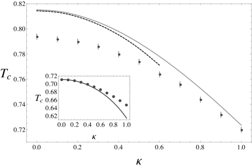
Figure 3.3: Main Figure: Critical temperature $T_{c}^{\kappa}$ vs nonextensive parameter $\kappa$ (points). The numerical results are based on an ensemble of 800 networks with $N=10^{3}$ nodes. The temperature for $\kappa=0.9$ is $(0.732\pm 0.002)$ and it is statistically compatible with the previous result $T_{c}^{\left(0.9\right)}=(0.73\pm 0.03)$ for an ensemble of 90 networks with $N=10000$. The upper bound $T_{c\kappa}^{*}+\Delta T$ is computed numerically (continuous line) and by using our analytical upper bound (dashed line). Inset: Numerically computed $T_{c\kappa}^{*}$ (dots) vs our analytical upper bound (continuous line). Because of the truncated McLaurin expansion, our approximation underestimates the critical temperature and breaks around $\kappa\sim 0.5$.

In order to compare our analytical findings with the numerical ones, we have to be aware of the finite size effects $\Delta T_{c}^{\kappa}$ in the numerical estimates for the critical temperatures $T_{c}^{\kappa}\simeq T_{c\kappa}^{*}+\Delta T$. Following the results in [6], the finite size correction $\Delta T_{c}^{\kappa}=\Delta T(N,T_{c\kappa}^{*})$ can be estimated with a first order series expansion from $I(\beta,\mu)$ at the critical point. One obtains:

$$\Delta T\simeq\frac{(T_{c\kappa}^{*})^{4}}{\ln N}\intop_{0}^{1}\frac{\epsilon^{2}e_{\kappa}^{\epsilon/T_{c\kappa}^{*}}}{(e_{\kappa}^{\epsilon/T_{c\kappa}^{*}}-1)^{2}}d\epsilon\;.$$

We notice that the analytical upper bound is in good agreement with numerical simulations for low values of $\kappa$. In agreement with the simulations we thus find that the critical temperature for the Bose-Einstein condensation decreases with $\kappa$. This is also compatible with a similar result derived in [14], under slightly less general assumptions on the functional form of the $\kappa$-deformed Bose-Einstein distribution.

All in all, it is interesting to note that the deformations inside the distribution $n_{\kappa}\left(\epsilon\right)$ do not influence the qualitative presence of the condensation, which is ultimately rooted in the properties of the energy density $g\left(\epsilon\right)$. These results suggest that the use of a nonextensive statistics, such as the Kaniadakis one, does not cause any qualitative change of the network dynamics. The main influence of a change from extensive to nonexstensive statistics are quantitative variations in the critical temperature. This observation is in agreement with the results of the numerical experiments reported in [10] for the Tsallis $q$-distribution. In order to further investigate this claim, we will proceed with the analysis of the degree distributions of our generalized fitness model in the next section.

3.2 Degree Distribution and Nonextensivity Parameter

In [4], the authors analyzed the degree distribution $P(k)$ of a fitness model with an exponential fitness distribution $\rho(\eta)$, obtaining the following estimate

$$P(k)\propto\int d\eta\rho(\eta)\frac{1}{F(\eta)}\left(\frac{m}{k}\right)^{F(\eta)^{-1}+1}$$ (3.3)

where $F(\eta)$ is the dynamical exponent which determines the growth of node degrees conditional on fitness. Using Eq. (2.5) $F(\eta)$ is to be identified with $f_{\kappa}\left(\epsilon\right)=e_{\kappa}^{\beta(\mu_{\kappa}\overset{\kappa}{\ominus}\epsilon)}$ in our generalized model. According to our definition of fitness $\eta$, given in Eq. (2.3), we have $e_{\kappa}^{-\beta\epsilon}=\eta$ and $e_{\kappa}^{\beta\mu}=z_{k}$ is the fugacity. Furthermore, $\rho(\eta)=\frac{1}{\beta}e_{\kappa}^{\beta\epsilon}g(\epsilon)$ is the distribution of fitnesses expressed in terms of the energy level distribution $g(\epsilon)$. These substitutions lead to:

$$P_{\kappa}(k)\propto\intop_{e_{\kappa}^{-\beta}}^{1}d\eta\left(-\frac{2}{\beta^{2}}\frac{\ln_{\kappa}\eta}{\eta}\right)\frac{1}{z_{\kappa}\eta}\left(\frac{m}{k}\right)^{1+\left(z_{\kappa}\eta\right)^{-1}}=$$ (3.4)

$$=\intop_{e_{\kappa}^{-\beta}}^{1}d\eta\left(-\frac{2}{\beta^{2}}\frac{\ln_{\kappa}\eta}{\eta}\right)\varphi_{\kappa,k}(\eta)=\mathbb{E}[\varphi_{\kappa,k}(\eta)]\;.$$

Even if the fictitious temperature in $\beta$ only plays the role of a control parameter of the model, it actually has some influence on the degree distribution, entering implicitly in the determination of the scaling exponent via $z_{\kappa}$ and also via the lower bound of fitness range.

$\varphi_{\kappa,k}(x)$ is a convex function for $\eta\in[e_{\kappa}^{-\beta},1]$ when $k>16$ and making use of Jensen’s inequality one finds

$$\mathbb{E}[\varphi_{\kappa,k}(\eta)]\geq\varphi_{\kappa,k}\left(\mathbb{E}[\eta]\right)=\frac{1}{z_{\kappa}\mathbb{E}[\eta]}\left(\frac{m}{k}\right)^{1+\left(z_{\kappa}\mathbb{E}[\eta]\right)^{-1}}\;.$$ (3.5)

By using the definition of the $\kappa$-deformed logarithm given in Eq. (2.1) one can now compute the expected value of the fitness $\mathbb{E}[\eta]$ which is a monotonically increasing function of the temperature for every $\kappa\in(0,1]$:

$$\mathbb{E}[\eta]=\frac{1}{\kappa\beta^{2}}\left[\frac{1}{\kappa+1}(e_{\frac{\kappa}{\kappa+1}}^{-\beta(\kappa+1)}-1)+\frac{1}{\kappa-1}(e_{\frac{\kappa}{1-\kappa}}^{-\beta(1-\kappa)}-1)\right]\;.$$ (3.6)

The arguments above motivate our estimate for the degree distribution of a generalized fitness network with a logarithmic distribution of fitnesses over a finite range, in terms of a lower bound given by a power law:

$$P_{\kappa}(k)\sim\frac{1}{z_{\kappa}\mathbb{E}[\eta]}\left(\frac{m}{k}\right)^{1+\left(z_{\kappa}\mathbb{E}[\eta]\right)^{-1}}$$ (3.7)

with the exponent $\gamma_{\kappa,T}=1+\left(z_{\kappa}\mathbb{E}[\eta]\right)^{-1}$ implicitly dependent on network temperature and on the nonextensive parameter $\kappa$. The fugacity $z_{\kappa}$ can be determined using Eq. (2.7).

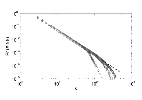
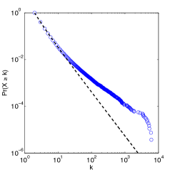
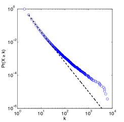
Figure 3.4: Complementary cumulative distribution functions $P(x\geq k)$ for the degree distribution in a network with $N$ nodes for different values of temperature and nonextensive parameter. Upper Centre:$\kappa=0.9$ and $T=5$ for $N=10^{3}$ (crosses), $N=5\cdot 10^{3}$ (squares) and $N=10^{4}$. The dashed straight line is a power law with exponent $\gamma=3$, for reference. The data shows a power-law like behavior with a cut-off depending on the system finite size. Lower Left: $\kappa=0.2$ and $T=0.5$. Lower Right: $\kappa=0.9$ and $T=0.5$. The dashed line is the estimate based on a power-law assumption, with scaling exponents respectively $\gamma_{0.2,0.5}\simeq 2.86$ and $\gamma_{0.9,0.5}\simeq 2.79$. Notice that the first part of the plot is robust to temperature changes, as confirmed by the retrieved scaling exponents. Lowering the temperature stretches the distribution only in the higher degree zone.

Numerical simulations of degree distributions show a good level of agreement with the power-law estimate. In the “fit-get-rich” phase ($T=5>T_{c}^{\left(\kappa\right)}\,\forall\kappa\in[0,1]$) three ensembles of 100 networks of sizes $N=\{10^{3},5\cdot 10^{3},10^{4}\}$ clearly display power-law like behavior with a finite-size cut off. Similar results were cited for upper bounded fitness distributions in [4].

In Figure 3.4 a maximum likelihood fitting procedure [19] reveals scaling exponents for the power-law like parts of the plots statistically compatible with the value $\gamma_{0.2,5}=2.89\pm 0.05$ for the ensemble with $N=10^{4}$ and $\kappa=0.9$. Other scaling exponents for lower values of $\kappa$ were retrieved, all close to the exponent ($\simeq 3$) estimated from our analytical upper bound in Eq. (3.7). The maximum-likelihood procedure we used avoids biases generated by adopting a linear binning scheme, which could potentially alter or masque the stretched-exponential region. Our estimate for the scaling parameter is suprisingly close to the one for a growing network with preferential attachment [15, 3], which is recovered by the generalized model either with the choice $\rho(\eta)=\delta(\eta-\eta_{0})$ or in the limit $T\rightarrow+\infty$ (in both cases, every node has the same fitness). Furthermore, in the limit $T\rightarrow\infty$ the $\kappa$-deformed exponential for the fitnesses recovers the Boltzmann weight, in which case it can be shown analytically that $1/z_{\kappa}\rightarrow 1/z\rightarrow 2$ while in the same limit $T\rightarrow\infty$ the average fitness for our model converges to 1, so that the scaling parameter recovers our numerical estimate

$$\gamma_{\kappa,T}\overset{T\rightarrow\infty}{\rightarrow}3\,\forall\kappa\in[0,1].$$ (3.8)

Nonetheless, in [4], it was shown that the fitness model is not stable under changes of the functional form of the fitness distribution function: The model can give rise to power laws (uniform $\rho(\eta)$) or non power-law degree distributions (unbounded exponential distributions $\rho(\eta)$).

In the high temperature region $T\gg T_{c}^{\left(\kappa\right)}$, numerical experiments for the fugacity $z_{\kappa}$, performed on an ensenmble of 800 networks with $N=10^{3}$, suggest that our estimate $\gamma_{\kappa,T}$ is effectively independent of both the temperature and the nonextensive parameter, with $\gamma_{\kappa,T}=\gamma^{*}\simeq 3$. This finding agrees with the boundary condition that $\gamma_{\kappa,T}\rightarrow 3$ for $T\rightarrow+\infty$ and $\forall\kappa\in[0,1]$ (as stated above, our model degenerates into the Barabási-Albert model). Instead, in the low temperature phase $T\ll T_{c}^{\kappa}$, any numerical computation of the fugacity $z_{\kappa}$ suffers from finite size-effects, but theoretical arguments put forward in [6] lead to an estimate of $z_{\kappa}\simeq 1$ also for the nonextensive case, since $e_{\kappa}^{x}\sim e^{x}$ when $x\ll 1$. Given that the average fitness $\mathbb{E}(\eta)$ monotonically decreases to $0$ when the temperature decreases, then from Eq. (3.7) the scaling exponent $\gamma_{\kappa,T}$ has to increase when $T$ decreases, depending on the nonextensive parameter $\kappa$. Nonetheless, as the lower bound in (3.5) is valid only for degrees $k>k_{0}$, only a part of the points on the $P(k)$ plot is shifted and raised from the original behavior, at high degrees, and the result is a stretched exponential, compatible with those shown in 3.4.

Furthermore, as reported in [6], an accurate theoretical analysis of the network dynamics in the condensate phase for the original BB model $g(\epsilon)=2\epsilon,\,\epsilon\in(0,1)$ found evidence for not only one “gel” node [18], (i.e. one unique condensate) but for an infinite hierarchy of condensates, whose degrees grow faster than $F(\eta)$ and linearly with time. A similar picture, in which there is not one unique “winner”, was also presented in [16].

This phenomenon is due to the presence of a crossover timescale $\tau(T)\sim T^{-2}$ in the condensate phase. The “winner-takes-all” phenomenon occurs only for networks having evolved for times greater than $\tau(T)$, which diverges at low temperature. For shorter times, a record-driven dynamics [16] is observed instead, with the number $D(t)$ of candidate “gel” nodes up to time $t$ growing as $D(t)\sim 2\ln\ln t$ [6]. These super-hubs, which sum up to the condensed fraction $1-I_{\beta}$, escape our mean-field approach, in which $k_{i}$ has to grow sublinearly in time, according to Eq. (2.5). Ultimately, it is those hubs which give rise to the stretched exponential encountered in our numerical experiments in the condensate phase.

4 Conclusions

In this paper we have generalized the Barabási-Bianconi fitness model by the means of the non-Gaussian Kaniadakis $\kappa$-distribution, which was originally proposed in the framework of nonextensive statistical mechanics. Our analytical results show that the resulting generalized fitness model presents a phase transition from a “fit-get-rich” phase to a “gel” phase, formally equivalent to a Bose-Einstein condensation. Analytical calculations supported by numerical estimates show that the critical temperature $T_{c}$ of the Bose-Einstein condensation on networks decreases when the nonextensive parameter $\kappa$ is increased from $0$ to $1$. A numerical analysis of the degree distribution, complemented by an analytically obtained lower bound, reveals the presence of power-law behaviour in the phase of high-temperatures and a linear energy level density for $g(\epsilon)\rightarrow 0$. In contrast, in the condensate phase stretched exponentials, compatible with the recent finding of a hierarchy of hubs, are retrieved.

5 Acknowledgements

MS is personally indebted to Prof. P. Tempesta and Prof. R. A. Leo for the precious insights they provided. Without the latter, this article would not have been written. MS is also grateful to Clément Viguier and the whole Complex Systems Simulation DTC at the Institute of Complex Systems Simulation (ICSS), University of Southampton, for their support. MS and MB also acknowledge the use of both MATLAB code written by Aaron Clauset, from [19], and of the IRIDIS High Performance Computing Facility, and associated support services at the University of Southampton, in the completion of this work.

References

- [1] M. E. J. Newman, “The structure and function of complex networks,” SIAM Review, vol. 45, pp. 167–256, 2003.
- [2] G. Caldarelli, Scale-Free Networks. Oxford University Press, 2007.
- [3] R. Albert and A.-L. Barabási, “Statistical mechanics of complex networks,” Reviews of Modern Physics, vol. 74, no. 1, pp. 47–97, 2002.
- [4] G. Bianconi and A.-L. Barabási, “Competition and multiscaling in evolving networks,” EPL (Europhysics Letters), vol. 54, no. 4, pp. 436–442, 2001.
- [5] G. Bianconi and A. L. Barabási, “Bose-Einstein condensation in complex networks,” Physical Review Letters, vol. 86, no. 24, pp. 5632–5635, 2001.
- [6] C. Godréche and J. M. Luck, “On leaders and condensates in a growing network,” Journal of Statistical Mechanics: Theory and Experiment, vol. 2010, no. 07, p. P07031, 2010.
- [7] C. Tsallis, Introduction to Nonextensive Statistical Mechanics - Approaching a Complex World. Springer, 2009.
- [8] F. Clementi, M. Gallegati, and G. Kaniadakis, “A new model of income distribution: the k-generalized distribution,” Journal of Economics, vol. 105, no. 1, pp. 63–91, 2012.
- [9] S. Thurner and R. Hanel, “The entropy of non-ergodic complex systems: a derivation from first principles,” International Journal of Modern Physics: Conference Series, vol. 16, pp. 105–115, 2012.
- [10] G. Su, X. Zhang, and Y. Zhang, “Tsallis mapping in growing complex networks with fitness,” Communications in Theoretical Physics, vol. 57, no. 3, p. 493, 2012.
- [11] G. Kaniadakis, “Statistical mechanics in the context of special relativity,” Physical Review E, vol. 66, no. 5, p. 056125, 2002.
- [12] J. C. Carvalho, J. D. do Nascimento, R. Silva, and J. R. D. Medeiros, “Non-gaussian statistics and stellar rotational velocities of main-sequence field stars,” The Astrophysical Journal Letters, vol. 696, no. 1, p. L48, 2009.
- [13] A. M. Teweldeberhan, H. G. Miller, and R. Tegen, “k-deformed statistics and the formation of a quark-gluon plasma,” International Journal of Modern Physics E, vol. 12, no. 05, pp. 669–673, 2003.
- [14] A. Aliano, G. Kaniadakis, and E. Miraldi, “Bose-Einstein condensation in the framework of k-statistics,” Physica B: Condensed Matter, vol. 325, pp. 35–40, 2003.
- [15] A. L. Barabási and R. Albert, “Emergence of scaling in random networks,” Science, vol. 286, no. 5439, pp. 509–512, 1999.
- [16] L. Ferretti and G. Bianconi, “Dynamics of condensation in growing complex networks,” Physical Review E, vol. 78, no. 5, p. 056102, 2008.
- [17] G. Kaniadakis, “Maximum entropy principle and power-law tailed distributions,” The European Physical Journal B, vol. 70, pp. 3–13, 2009.
- [18] P. L. Krapivsky, S. Redner, and F. Leyvraz, “Connectivity of growing random networks,” Physical Review Letters, vol. 85, pp. 4629–4632, 2000.
- [19] A. Clauset, C. Shalizi, and M. Newman, “Power-law distributions in empirical data,” SIAM Review, vol. 51, no. 4, pp. 661–703, 2009.