Efficient Inference and Learning in a Large Knowledge Base

Abstract

One important challenge for probabilistic logics is reasoning with very large knowledge bases (KBs) of imperfect information, such as those produced by modern web-scale information extraction systems. One scalability problem shared by many probabilistic logics is that answering queries involves “grounding” the query—i.e., mapping it to a propositional representation—and the size of a “grounding” grows with database size. To address this bottleneck, we present a first-order probabilistic language called ProPPR in which that approximate “local groundings” can be constructed in time independent of database size. Technically, ProPPR is an extension to stochastic logic programs (SLPs) that is biased towards short derivations; it is also closely related to an earlier relational learning algorithm called the path ranking algorithm (PRA). We show that the problem of constructing proofs for this logic is related to computation of personalized PageRank (PPR) on a linearized version of the proof space, and using on this connection, we develop a proveably-correct approximate grounding scheme, based on the PageRank-Nibble algorithm. Building on this, we develop a fast and easily-parallelized weight-learning algorithm for ProPPR. In experiments, we show that learning for ProPPR is orders magnitude faster than learning for Markov logic networks; that allowing mutual recursion (joint learning) in KB inference leads to improvements in performance; and that ProPPR can learn weights for a mutually recursive program with hundreds of clauses, which define scores of interrelated predicates, over a KB containing one million entities.

1 Introduction

While probabilistic logics are useful for many important tasks (Lowd and Domingos, 2007; Fuhr, 1995; Poon and Domingos, 2007, 2008); in particular, such logics would seem to be well-suited for inference with the “noisy” facts that are extracted by automated systems from unstructured web data. While some positive results have been obtained for this problem (Cohen, 2000), most probabilistic first-order logics are not efficient enough to be used for inference on the very large broad-coverage KBs that modern information extraction systems produce (Suchanek et al, 2007; Carlson et al, 2010). One key problem is that queries are typically answered by “grounding” the query—i.e., mapping it to a propositional representation, and then performing propositional inference—and for many logics, the size of the “grounding” can be extremely large for large databases. For instance, in probabilistic Datalog (Fuhr, 1995), a query is converted to a structure called an “event expression”, which summarizes all possible proofs for the query against a database; in ProbLog (De Raedt et al, 2007) and MarkoViews (Jha and Suciu, 2012) similar structures are created, encoded more compactly with binary decision diagrams (BDDs); in probabilistic similarity logic (PSL) an intentional probabilistic program, together with a database, is converted to constraints for a convex optimization problem; and in Markov Logic Networks (MLNs) (Richardson and Domingos, 2006), queries are converted to a (propositional) Markov network. In all of these cases, the result of this “grounding” process can be large.

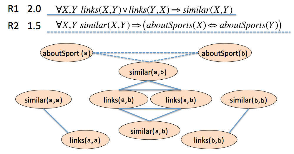
Figure 1: A Markov logic network program and its grounding relative to two constants $a,b$. (Dotted lines are clique potentials associated with rule R2, solid lines with rule R1.)

As concrete illustration of the “grounding” process, Figure 1 shows a very simple MLN and its grounding over a universe of two web pages $a$ and $b$. (Here the grounding is query-independent.). In MLNs, the result of the grounding is a Markov network which contains one node for every atom in the Herbrand base of the program—i.e., the number of nodes is $O(n^{k})$ where $k$ is the maximal arity of a predicate and $n$ the number of database constants. However, even a grounding of size that is only linear in the number of facts in the database, $|DB|$, would impractically large for inference on real-world problems. Superficially, it would seem that groundings must inherently be $o(|DB|)$ for some programs: in the example, for instance, the probability of aboutSport(x) must depend to some extent on the entire hyperlink graph (if it is fully connected). However, it also seems intuitive that if we are interested in inferring information about a specific page—say, the probability of aboutSport(d1)—then the parts of the network only distantly connected to d1 are likely to have a small influence. This suggests that an approximate grounding strategy might be feasible, in which a query such as aboutSport(d1) would be grounded by constructing a small subgraph of the full network, followed by inference on this small “locally grounded” subgraph. Likewise, consider learning (e.g., from a set of queries $Q$ with their desired truth values). Learning might proceed by locally-grounding every query goal, allowing learning to also take less than $O(|DB|)$ time.

In this paper, we present a first-order probabilistic language which is well-suited to such approximate “local grounding”. We describe an extension to stochastic logic programs (SLP) (Cussens, 2001) that is biased towards short derivations, and show that this is related to personalized PageRank (PPR) (Page et al, 1998; Chakrabarti, 2007) on a linearized version of the proof space. Based on the connection to PPR, we develop a proveably-correct approximate inference scheme, and an associated proveably-correct approximate grounding scheme: specifically, we show that it is possible to prove a query, or to build a graph which contains the information necessary for weight-learning, in time $O(\frac{1}{\alpha\epsilon})$, where $\alpha$ is a reset parameter associated with the bias towards short derivations, and $\epsilon$ is the worst-case approximation error across all intermediate stages of the proof. This means that both inference and learning can be approximated in time independent of the size of the underlying database—a surprising and important result, which leads to a very scalable inference algorithm.

The ability to locally ground queries has another important consequence: it is possible to decompose the problem of weight-learning to a number of moderate-size subtasks (in fact, tasks of size $O(\frac{1}{\alpha\epsilon})$ or less) which are weakly coupled. Based on this we outline a parallelization scheme, which in our current implementation provides an order-of-magnitude speedup in learning time on a multi-processor machine.

Below, we will first introduce our formalism, and then describe our weight-learning algorithm. We next present experimental results on some small benchmark inference tasks. We then present experimental results on a larger, more realistic task: learning to perform accurate inference in a large KB of facts extracted from the web (Lao et al, 2011). We finally discuss related work and conclude.

2 Programming with Personalized PageRank (PROPPR)

2.1 Inference as Graph Search

We will now describe our “locally groundable” first-order probabilistic language, which we call ProPPR. Inference for ProPPR is based on a personalized PageRank process over the proof constructed by Prolog’s Selective Linear Definite (SLD) resolution theorem-prover. To define the semantics we will use notation from logic programming (Lloyd, 1987). Let $LP$ be a program which contains a set of definite clauses $c_{1},\ldots,c_{n}$, and consider a conjunctive query $Q$ over the predicates appearing in $LP$. A traditional Prolog interpreter can be viewed as having the following actions. First, construct a “root vertex” $v_{0}$, which is a pair $(Q,Q)$ and add it to an otherwise-empty graph $G^{\prime}_{Q,LP}$. (For brevity, we drop the subscripts of $G^{\prime}$ where possible.) Then recursively add to $G^{\prime}$ new vertices and edges as follows: if $u$ is a vertex of the form $(Q,(R_{1},\ldots,R_{k}))$, and $c$ is a clause in $LP$ of the form $R^{\prime}\leftarrow S^{\prime}_{1},\ldots,S^{\prime}_{\ell}$, and $R_{1}$ and $R^{\prime}$ have a most general unifier $\theta=mgu(R_{1},R^{\prime})$, then add to $G^{\prime}$ a new edge ${{u\rightarrow{}v}}$ where $v=(Q\theta,(S^{\prime}_{1},\ldots,S^{\prime}_{\ell},R_{2},\ldots,R_{k})\theta)$. Let us call $Q\theta$ the transformed query and $(S^{\prime}_{1},\ldots,S^{\prime}_{\ell},R_{2},\ldots,R_{k})\theta$ the associated subgoal list. If a subgoal list is empty, we will denote it by $\Box$. Here $Q\theta$ denotes the result of applying the substitution $\theta$ to $Q$; for instance, if $Q=about(a,Z)$ and $\theta=\{Z=fashion\}$, then $Q\theta$ is $about(a,fashion)$.

The graph $G^{\prime}$ is often large or infinite so it is not constructed explicitly. Instead Prolog performs a depth-first search on $G^{\prime}$ to find the first solution vertex $v$—i.e., a vertex with an empty subgoal list—and if one is found, returns the transformed query from $v$ as an answer to $Q$.

Table 1 and Figure 2 show a simple Prolog program and a proof graph for it. The annotations after the hashmarks and the edge labels in the proof graph will be described below in more detail: briefly, however, we will associated with each use of a clause $c$ a feature vector $\phi$, which is computed from the binding to the variables in the head of $c$. For instance, applying the clause “sim(X,Y):-links(X,Y)” always yields a vector $\phi$ that has unit weight on (the dimensions corresponding to) the two ground atoms sim and link, and zero weight elsewhere; likewise, applying the clause “linkedBy(X,Y),W:-” to the goal linkedBy(a,c,sprinter) yields a vector $\phi$ that has unit weight on the atom by(sprinter).

For conciseness, in Figure 2 only the subgoals $R_{1},\ldots,R_{k}$ are shown in each node $u=(Q,(R_{1},\ldots,R_{k}))$. Given the query $Q=\textit{about(a,Z)}$, Prolog’s depth-first search would return $Q=\textit{about(a,fashion)}$. Note that in this proof formulation, the nodes are conjunctions of literals, and the structure is, in general, a digraph (rather than a tree). Also note that the proof is encoded as a graph, not a hypergraph, even if the predicates in the LP are not binary: the edges represent a step in the proof that reduces one conjunction to another, not a binary relation between entities.

Table 1: A simple program in ProPPR. See text for explanation.

about(X,Z) :- handLabeled(X,Z)	# base.
about(X,Z) :- sim(X,Y),about(Y,Z)	# prop.
sim(X,Y) :- links(X,Y)	# sim,link.
sim(X,Y) :-
hasWord(X,W),hasWord(Y,W),
linkedBy(X,Y,W)	# sim,word.
linkedBy(X,Y,W) :- true	# by(W).

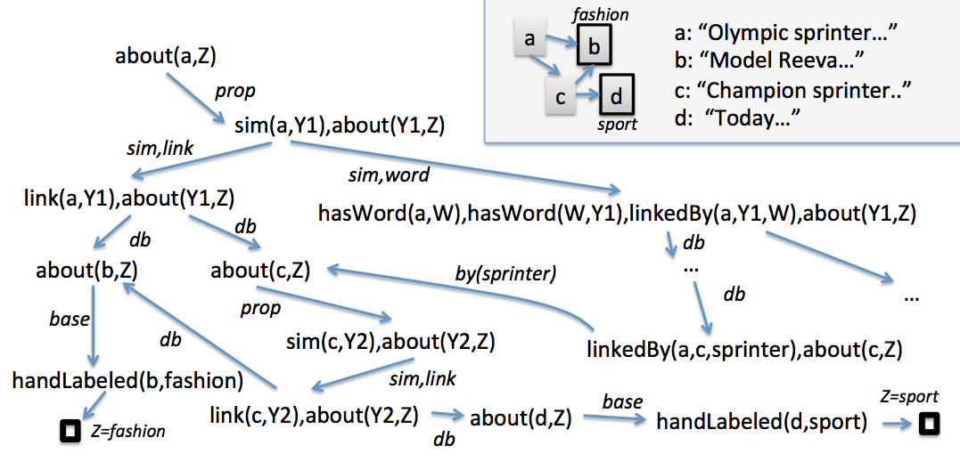
Figure 2: A partial proof graph for the query about(a,Z). The upper right shows the link structure between documents $a,b,c$, and $d$, and some of the words in the documents. Restart links are not shown.

As an further illustration of the sorts of ProPPR programs that are possible, some small sample programs are shown in Figure 2. Clauses $c_{1}$ and $c_{2}$ are, together, a bag-of-words classifier: each proof of predictedClass(D,Y) adds some evidence for $D$ having class $Y$, with the weight of this evidence depending on the weight given to $c_{2}$’s use in establishing related(w,y), where $w$ and $y$ are a specific word in $D$ and $y$ is a possible class label. In turn, $c_{2}$’s weight depends on the weight assigned to the $r(w,y)$ feature by w, relative to the weight of the restart link. Adding $c_{3}$ and $c_{4}$ to this program implements label propagation, and adding $c_{5}$ and $c_{6}$ implements a sequential classifier. These examples show that ProPPR allows many useful heuristics to be encoded as programs.

Table 2: Some more sample ProPPR programs. $LP=\{c_{1},c_{2}\}$ is a bag-of-words classifier (see text). $LP=\{c_{1},c_{2},c_{3},c_{4}\}$ is a recursive label-propagation scheme, in which predicted labels for one document are assigned to similar documents, with similarity being an (untrained) cosine distance-like measure. $LP=\{c_{1},c_{2},c_{5},c_{6}\}$ is a sequential classifier for document sequences.

$c_{1}$:	pred	ictedClass(Doc,Y) :-
		possibleClass(Y),
		hasWord(Doc,W),
		related(W,Y) # c1.
$c_{2}$: related(W,Y) :- true,
	# relatedFeature(W,Y)
Database predicates:
hasWord(D,W): doc $D$ contains word $W$
inDoc(W,D): doc $D$ contains word $W$
previous(D1,D2): doc $D2$ precedes $D1$
possibleClass(Y): $Y$ is a class label

$c_{3}$:	pre	dictedClass(Doc,Y) :-
		similar(Doc,OtherDoc),
		predictedClass(OtherDoc,Y) # c3.
$c_{4}:$ similar(Doc1,Doc2) :-
		hasWord(Doc1,W),
		inDoc(W,Doc2) # c4.
$c_{5}:$ predictedClass(Doc,Y) :-
		previous(Doc,OtherDoc),
		predictedClass(OtherDoc,OtherY),
		transition(OtherY,Y) # c5.
$c_{6}$: transition(Y1,Y2) :- true,
	# transitionFeature(Y1,Y2)

2.2 From SLPs to ProPPR

In stochastic logic programs (SLPs) (Cussens, 2001), one defines a randomized procedure for traversing the graph $G^{\prime}$, which thus defines a probability distribution over vertices $v$, and hence (by selecting only solution vertices) a distribution over transformed queries (i.e. answers) $Q\theta$. The randomized procedure thus produces a distribution over possible answers, which can be tuned by learning to upweight desired (correct) answers and downweight others.

In past work, the randomized traversal of $G^{\prime}$ was defined by a probabilistic choice, at each node, of which clause to apply, based on a weight for each clause. We propose two extensions. First, we will introduce a new way of computing clause weights, which allows for a potentially richer parameterization of the traversal process. We will associate with each edge ${{u\rightarrow{}v}}$ in the graph a feature vector $\phi_{{{u\rightarrow{}v}}}$. This edge is produced indirectly, by associating with every clause $c\in{}LP$ a function $\Phi_{c}(\theta)$, which produces the vector $\phi$ associated with an application of $c$ using mgu $\theta$. As an example, if the last clause of the program in Table 1 was applied to $(Q,linkedBy(a,c,sprinter),about(c,Z))$ with mgu $\theta=\{X=a,Y=c,W=sprinter\}$ then $\Phi_{c}(\theta)$ would be $\{by(sprinter)\}$, if we use a set to denote a sparse vector with 0/1 weights.

This feature vector is computed during theorem-proving, and used to annotate the edge ${{u\rightarrow{}v}}$ in $G^{\prime}$ created by applying $c$ with mgu $\theta$. Finally, an edge ${{u\rightarrow{}v}}$ will be traversed with probability $\Pr(v|u)\propto f(\textbf{w},\phi_{{u\rightarrow{}v}})$ where w is a parameter vector and where $f(\textbf{w},\phi)$ is a weighting function. (Here we use $f(\textbf{w},\phi)=\exp(\textbf{w}_{i}\cdot\phi)$, but any differentiable function would be possible.) This weighting function now determines the probability of a transition, in theorem-proving, from $u$ to $v$: specifically, $\Pr_{\textbf{w}}(v|u)\propto f(\textbf{w},\phi_{{u\rightarrow{}v}})$. Weights in w default to 1.0, and learning consists of tuning these weights.

The second and more fundamental extension is to add edges in $G^{\prime}$ from every solution vertex to itself, and also add an edge from every vertex to the start vertex $v_{0}$. We will call this augmented graph $G_{Q,LP}$ below (or just $G$ if the subscripts are clear from context). These links make SLP’s graph traversal a personalized PageRank (PPR) procedure, sometimes known as random-walk-with-restart (Tong et al, 2006). These links are annotated by another feature vector function $\Phi_{\mathrm{restart}}(R)$, which is applied to the leftmost literal $R$ of the subgoal list for $u$ to annotate the edge ${u\rightarrow{}v}_{0}$.

These links back to the start vertex bias the traversal of the proof graph to upweight the results of short proofs. To see this, note that if the restart probability $P(v_{0}|u)=\alpha$ for every node $u$, then the probability of reaching any node at depth $d$ is bounded by $(1-\alpha)^{d}$.

To summarize, if $u$ is a node of the search graph, $u=(Q\theta,(R_{1},\ldots,R_{k}))$, then the transitions from $u$, and their respective probabilities, are defined as follows, where $Z$ is an appropriate normalizing constant:

• If $v=(Q\theta\sigma,(S^{\prime}_{1},\ldots,S^{\prime}_{\ell},R2,\ldots,R_{k})\theta\sigma)$ is a state derived by applying the clause $c$ (with mgu $\sigma$), then

  $$\Pr_{\textbf{w}}(v|u)=\frac{1}{Z}f(\textbf{w},\Phi_{c}(\theta\circ\sigma))$$

• If $v=v_{0}=(Q,Q)$ is the initial state in $G$, then

  $$\Pr_{\textbf{w}}(v|u)=\frac{1}{Z}f(\textbf{w},\Phi_{\mathrm{restart}}(R_{1}\theta))$$

• If $v$ is any other node, then $\Pr(v|u)=0$.

Finally we must specify the functions $\Phi_{c}$ and $\Phi_{\mathrm{restart}}$. For clauses in $LP$, the feature-vector producing function $\Phi_{c}(\theta)$ for a clause is specified by annotating $c$ as follows: every clause $c=(R\leftarrow S_{1},\ldots,S_{k})$ can be annotated with an additional conjunction of “feature literals” $F_{1},\ldots,F_{\ell}$, which are written at the end of the clause after the special marker “#”. The function $\Phi_{c}(\theta)$ then returns a vector $\phi=\{F_{1}\theta,\ldots,F_{\ell}\theta\}$, where every $F_{i}\theta$ must be ground.

The requirement that edge features $F_{i}\theta$ are ground is the reason for introducing the apparently unnecessary predicate linkedBy(X,Y,W) into the program of Table 1: adding the feature literal by(W) to the second clause for sim would result in a non-ground feature by(W), since $W$ is a free variable when $\Phi_{c}$ is called. Notice also that the weight on the by(W) features are meaningful, even though there is only one clause in the definition of linkedBy, as the weight for applying this clause competes with the weight assigned to the restart edges.

It would be cumbersome to annotate every database fact, and difficult to learn weights for so many features. Thus, if $c$ is the unit clause that corresponds to a database fact, then $\Phi_{c}(\theta)$ returns a default value $\phi=\{\textit{db}\}$, where db is a special feature indicating that a database predicate was used.

The function $\Phi_{\mathrm{restart}}(R)$ depends on the functor and arity of $R$. If $R$ is defined by clauses in $LP$, then $\Phi_{\mathrm{restart}}(R)$ returns a unit vector $\phi=\{\textit{defRestart}\}$. If $R$ is a database predicate (e.g., hasWord(doc1,W)) then we follow a slightly different procedure, which is designed to ensure that the restart link has a reasonably large weight even with unit feature weights: we compute $n$, the number of possible bindings for $R$, and set $\phi[\textit{defRestart}]=n\cdot{}\frac{\alpha}{1-\alpha}$, where $\alpha$ is a global parameter. This means that with unit weights, after normalization, the probability of following the restart link will be $\alpha$.

Putting this all together with the standard iterative approach to computing personalized PageRank over a graph (Page et al, 1998), we arrive at the following inference algorithm for answering a query $Q$, using a weight vector w. Below, we let $N_{v_{0}}(u)$ denote the neighbors of $u$—i.e., the set of nodes $v$ where $\Pr(v|u)>0$ (including the restart node $v=v_{0}$). We also let W be a matrix such that $\textbf{W}[u,v]=\Pr_{\textbf{w}}(v|u)$, and in our discussion, we use $\textbf{ppr}(v_{0})$ to denote the personalized PageRank vector for $v_{0}$.

1. Let $v_{0}=(Q,Q)$ be the start node of the search graph. Let $G$ be a graph containing just $v_{0}$. Let $\textbf{v}^{0}=\{v_{0}\}$.

2. For $t=1,\ldots,T$ (i.e., until convergence):

   • For each $u$ with non-zero weight in $\textbf{v}^{t-1}$, and each $v\in{}N_{u+0}(u)$, add $(u,v,\phi_{{{u\rightarrow{}v}}})$ to $G$ with weight $\Pr_{\textbf{w}}(v|u)$, and set $\textbf{v}^{t}=\textbf{W}\cdot\textbf{v}^{t-1}$

3. At this point $\textbf{v}^{T}\approx\textbf{ppr}(v_{0})$. Let $S$ be the set of nodes $(Q\theta,\Box)$ that have empty subgoal lists and non-zero weight in $\textbf{v}^{T}$, and let $Z=\sum_{u\in{}S}\textbf{v}^{T}[u]$. The final probability for the literal $L=Q\theta$ is found by extracting these solution nodes $S$, and renormalizing:

   $$\Pr_{\textbf{w}}(L)\equiv\frac{1}{Z}\textbf{v}^{T}[(L,\Box)]$$

For example, given the query $Q=\textit{about(a,Z)}$ and the program of Table 1, this procedure would give assign a non-zero probability to the literals about(a,sport) and about(a,fashion), concurrently building the graph of Figure 2.

Thus far, we have introduced a language quite similar to SLPs. The power-iteration PPR computation outlined above corresponds to a depth-bounded breadth-first search procedure, and the main extension of ProPPR, relative to SLPs, is the ability to label a clause application with a feature vector, instead of the clause’s identifier. Below, however, we will discuss a much faster approximate grounding strategy, which leads to a novel proof strategy, and a parallelizable weight-learning method.

2.3 Locally Grounding a Query

Table 3: The PageRank-Nibble-Prove algorithm for inference in ProPPR. $\alpha^{\prime}$ is a lower-bound on $\Pr(v_{0}|u)$ for any node $u$ to be added to the graph $\hat{G}$, and $\epsilon$ is the desired degree of approximation.

define PageRank-Nibble-Prove($Q$):
	let $\textbf{v}=$PageRank-Nibble$((Q,Q),\alpha^{\prime},\epsilon)$
	let $S=\{u:\textbf{p}[u]>u\mbox{~{}and~{}}u=(Q\theta,\Box)\}$
	let $Z=\sum_{u\in S}\textbf{p}[u]$
	define $\Pr_{\textbf{w}}(L)\equiv\frac{1}{Z}\textbf{v}[(L,\Box)]$
end
define PageRank-Nibble($v_{0},\alpha^{\prime},\epsilon$):
	let $\textbf{p}=\textbf{r}=\textbf{0}$, let $\textbf{r}[v_{0}]=1$, and let $\hat{G}=\emptyset$
	while $\exists u:\textbf{r}(u)/|N(u)|>\epsilon$ do:
		push($u$)
	return p
end

define push($u,\alpha^{\prime}$):
	comment: this modifies p, r, and $\hat{G}$
	$\textbf{p}[u]=\textbf{p}[u]+\alpha^{\prime}\cdot\textbf{r}[u]$
	$\textbf{r}[u]=\textbf{r}[u]\cdot(1-\alpha^{\prime})$
	for $v\in{}N(u)$:
		add the edge $(u,v,\phi_{{{u\rightarrow{}v}}})$ to $\hat{G}$
		if $v=v_{0}$ then
			$\textbf{r}[v]=\textbf{r}[v]+\Pr(v|u)\textbf{r}[u]$
		else
			$\textbf{r}[v]=\textbf{r}[v]+{(\Pr(v|u)-\alpha^{\prime})}\textbf{r}[u]$
	endfor
end

Note that this procedure both performs inference (by computing a distribution over literals $Q\theta$) and “grounds” the query, by constructing a graph $G$. ProPPR inference for this query can be re-done efficiently, by running an ordinary PPR process on $G$. This is useful for faster weight learning. Unfortunately, the grounding $G$ can be very large: it need not include the entire database, but if $T$ is the number of iterations until convergence for the sample program of Table 1 on the query $Q=about(d,Y)$, $G$ will include a node for every page within $T$ hyperlinks of $d$.

To construct a more compact local grounding graph $G$, we adapt an approximate personalized PageRank method called PageRank-Nibble (Andersen et al, 2006, 2008). This method has been used for the problem of local partitioning: in local partitioning, the goal is to find a small, low-conductance component $\hat{G}$ of a large graph $G$ that contains a given node $v$.

The PageRank-Nibble-Prove algorithm is shown in Table 3. It maintains two vectors: p, an approximation to the personalized PageRank vector associated with node $v_{0}$, and r, a vector of “residual errors” in p. Initially, $\textbf{p}=\emptyset$ and $\textbf{r}=\{v_{0}\}$. The algorithm repeatedly picks a node $u$ with a large residual error $\textbf{r}[u]$, and reduces this error by distributing a fraction $\alpha^{\prime}$ of it to $\textbf{p}[u]$, and the remaining fraction back to $\textbf{r}[u]$ and $\textbf{r}[v_{1}],\ldots,\textbf{r}[v_{n}]$, where the $v_{i}$’s are the neighbors of $u$. The order in which nodes $u$ are picked does not matter for the analysis (in our implementation, we follow Prolog’s usual depth-first search as much as possible.) Relative to PageRank-Nibble, the main differences are the the use of a lower-bound on $\alpha$ rather than a fixed restart weight and the construction of the graph $\hat{G}$.

Although the result stated in Andersen et al holds only for directed graphs, it can be shown, following their proof technique, that after each push, $\textbf{p}+\textbf{r}=\textbf{ppr}(v_{0})$. It is also clear than when PageRank-Nibble terminates, then for any $u$, the error $\textbf{ppr}(v_{0})[u]-\textbf{p}[u]$ is bounded by $\epsilon{}|N(u)|$: hence, in any graph where $N(u)$ is bounded, a good approximation can be obtained. Additionally, we have the following efficiency bound:

Theorem 2.1 (Andersen,Chung,Lang)

Let $u_{i}$ be the $i$-th node pushed by PageRank-Nibble-Prove. Then,
$\sum_{i}|N(u_{i})|<\frac{1}{\alpha^{\prime}\epsilon}$.

This can be proved by noting that initially $||\textbf{r}||_{1}=1$, and also that $||\textbf{r}||_{1}$ decreases by at least $\alpha^{\prime}\epsilon|N(u_{i})|$ on the $i$-th push. As a direct consequence we have the following:

Corollary 1

The number of edges in the graph $\hat{G}$ produced by PageRank-Nibble-Prove is no more than $\frac{1}{\alpha^{\prime}\epsilon}$.

Importantly, the bound holds independent of the size of the full database of facts. The bound also holds regardless of the size or loopiness of the full proof graph, so this inference procedure will work for recursive logic programs.

We should emphasize that this approximation result holds for the individual nodes in the proof tree, not the answers $Q\theta$ to a query $Q$. Following SLPs, the probability of an answer $Q\theta$ is the sum of the weights of all solution nodes that are associated with $\theta$, so if an answer is associated with $n$ solutions, the error for its probability estimate with PageRank-Nibble-Prove may be as large as $n\epsilon$.

To summarize, we have outlined an efficient approximate proof procedure, which is closely related to personalized PageRank. As a side-effect of inference for a query $Q$, this procedure will create a ground graph $\hat{G}_{Q}$ on which personalized PageRank can be run directly, without any (relatively expensive) manipulation of first-order theorem-proving constructs such as clauses or logical variables. As we will see, this “locally grounded” graph will be very useful in learning weights w to assign to the features of a ProPPR program.

2.4 Learning for ProPPR

As noted above, inference for a query $Q$ in ProPPR is based on a personalized PageRank process over the graph associated with the SLD proof of a query goal $G$. More specifically, the edges ${{u\rightarrow{}v}}$ of the graph $G$ are annotated with feature vectors $\phi_{{{u\rightarrow{}v}}}$, and from these feature vectors, weights are computed using a parameter vector w, and finally normalized to form a probability distribution over the neighbors of $u$. The “grounded” version of inference is thus a personalized PageRank process over a graph with feature-vector annotated edges.

In prior work, Backstrom and Leskovec (Backstrom and Leskovec, 2011) outlined a family of supervised learning procedures for this sort of annotated graph. In the simpler case of their learning procedure, an example is a triple $(v_{0},u,y)$ where $v_{0}$ is a query node, $u$ is a node in in the personalized PageRank vector $\textbf{p}_{v_{0}}$ for $v_{0}$, $y$ is a target value, and a loss $\ell(v_{0},u,y)$ is incurred if $\textbf{p}_{v_{0}}[u]\not=y$. In the more complex case of “learning to rank”, an example is a triple $(v_{0},u_{+},u_{-})$ where $v_{0}$ is a query node, $u_{+}$ and $u_{-}$ are nodes in in the personalized PageRank vector $\textbf{p}_{v_{0}}$ for $v_{0}$, and a loss is incurred unless $\textbf{p}_{v_{0}}[u_{+}]\geq\textbf{p}_{v_{0}}[u_{-}]$. The core of Backstrom and Leskovic’s result is a method for computing the gradient of the loss on an example, given a differentiable feature-weighting function $f(\textbf{w},\phi)$ and a differentiable loss function $\ell$. The gradient computation is broadly similar to the power-iteration method for computation of the personalized PageRank vector for $v_{0}$. Given the gradient, a number of optimization methods can be used to compute a local optimum.

Instead of directly using the above learning approach for ProPPR, we decompose the pairwise ranking loss into a standard positive-negative log loss function. The training data $D$ is a set of triples $\{(Q^{1},P^{1},N^{1}),\ldots,(Q^{m},P^{m},N^{m})\}$ where each $Q^{k}$ is a query, $P^{k}=\langle Q\theta_{+}^{1},\ldots,Q\theta_{+}^{I}\rangle$ is a list of correct answers, and $N^{k}$ is a list $\langle Q\theta_{-}^{1},\ldots,Q\theta_{-}^{J}\rangle$ incorrect answers. We use a log loss with $L_{2}$ regularization of the parameter weights. Hence the final function to be optimized is

$$-\Bigg{(}\sum_{k=1}^{I}\log\textbf{p}_{v_{0}}[u_{+}^{k}]+\sum_{k=1}^{J}\log(1-\textbf{p}_{v_{0}}[u_{-}^{k}])\Bigg{)}+\mu||\textbf{w}||^{2}_{2}$$

To optimize this loss, we use stochastic gradient descent (SGD), rather than the quasi-Newton method of Backstrom and Leskovic. Weights are initialized to $1.0+\delta$, where $\delta$ is randomly drawn from $[0,0.01]$. We set the learning rate $\beta$ of SGD to be $\beta=\frac{\eta}{\mathrm{epoch}^{2}}$ where epoch is the current epoch in SGD, and $\eta$, the initial learning rate, defaults to 1.0.

We implemented SGD because it is fast and has been adapted to parallel learning tasks (Zinkevich et al, 2010; Niu et al, 2011b). Local grounding means that learning for ProPPR is quite well-suited to parallelization. The step of locally grounding each $Q^{i}$ is “embarassingly” parallel, as every grounding can be done independently. To parallelize the weight-learning stage, we use multiple threads, each of which computes the gradient over a single grounding $\hat{G}_{Q^{k}}$, and all of which accesses a single shared parameter vector w. The shared parameter vector is a potential bottleneck (Zinkevich et al, 2009); while it is not a severe one on moderate-size problems, contention for the parameters becomes increasingly important on the largest tasks we have experimented with

3 Inference in a Noisy KB

In this section, we first introduce the challenges of inference in a noisy KB, and a recently proposed statistical relational learning solution, then we show how one can apply our proposed locally grounding theory to improve this learning scheme.

3.1 Challenges of Inference in a Noisy KB

A number of recent efforts in industry (Singhal, 2012) and academia (Suchanek et al, 2007; Carlson et al, 2010; Hoffmann et al, 2011) have focused on automatically constructing large knowledge bases (KBs). Because automatically-constructed KBs are typically imperfect and incomplete, inference in such KBs is non-trivial.

We situate our study in the context of the NELL (Never Ending Language Learning) research project, which is an effort to develop a never-ending learning system that operates 24 hours per day, for years, to continuously improve its ability to read (extract structured facts from) the web (Carlson et al, 2010) NELL is given as input an ontology that defines hundreds of categories (e.g., person, beverage, athlete, sport) and two-place typed relations among these categories (e.g., athletePlaysSport(Athlete, Sport)), which it must learn to extract from the web. NELL is also provided a set of 10 to 20 positive seed examples of each such category and relation, along with a downloaded collection of 500 million web pages from the ClueWeb2009 corpus (Callan and Hoy, 2009) as unlabeled data, and access to 100,000 queries each day to Google’s search engine. NELL uses a multi-strategy semi-supervised multi-view learning method to iteratively grow the set of extracted “beliefs”.

This task is challenging for two reasons. First, the extensional knowledge, inference is based on, is not only incomplete, but also noisy, since its extracted imperfectly from the web. For example, a football team might be wrongly recognized as two separate entities, one with connections to its team members, and the other with a connection to its home stadium. Second, the size of inference problems are much larger than those of traditional logical programming tasks. Given the very large broad-coverage KBs that modern information extraction systems produce (Suchanek et al, 2007; Carlson et al, 2010), even a grounding of size that is only linear in the number of facts in the database, $|DB|$, would impractically large for inference on real-world problems.

Past work on first-order reasoning has sought to address the first problem by learning “soft” inference procedures, which are more reliable than “hard” inference rules, and address the second problem by learning restricted inference procedures. In the next sub-section, we will recap a recent development in solving these problems, and draws a connection to the ProPPR language.

3.2 Inference using the Path Ranking Algorithm (PRA)

Lao et al (2011) use the path ranking algorithm (PRA) to learn an “inference” procedure based on a weighted combination of “paths” through the KB graph. PRA is a relational learning system which generates (and appropriately weights) rules, which accurately infer new facts from the existing facts in the noisy knowledge base. As an illustration, PRA’s might learn rules such as those in Table 4, which correspond closely to Horn clauses, as shown in the Table.

PRA only considers rules which correspond to “paths”, or chains of binary, function-free predicates. Like ProPPR, PRA will weight some solutions to these paths are weighted more heavily than others: specifically, weights of the solutions to a PRA “path” are based on random-walk probabilities in the corresponding graph. For instance, the last clause of Table 4, which corresponds to the “path”

$$T\xrightarrow{\mbox{teamHasAthlete}}A\xrightarrow{\mbox{athletePlaysSport}}S$$

can be understood as follows:

1. Given a team $T$, construct a uniform distribution $\mathcal{A}$ of athletes such that $A\in{\mathcal{A}}$ is a athlete playing for team $T$.

2. Given ${\mathcal{A}}$, construct a distribution of sports ${\mathcal{S}}$ such that $S\in{\mathcal{S}}$ is played by $A$.

This final distribution ${\mathcal{S}}$ is the result: thus the path gives a weighted distribution over possible sports played by a team. For a one-clause program, this distribution corresponds precisely to the distribution produced by ProPPR.

More generally, the output of PRA corresponds roughly to a ProPPR program in a particular form—namely, the form

$$\begin{array}[]{l}p(S,T)\leftarrow r_{1,1}S,X_{1}),r_{1,2}(X_{1},X_{2}),\ldots,r_{1,k_{1}}(X_{k_{1}-1},T).\\ p(S,T)\leftarrow r_{2,1}(S,X_{1}),r_{2,2}(X_{1},X_{2}),\ldots,r_{2,k_{2}}(X_{k_{2}-1},T).\\ \vdots\\ \end{array}$$

where $p$ is the binary predicate being learned, and the $r_{i,j}$’s are other predicates defined in the database. (In Table 4, we emphasize that the $r_{i,j}$’s are already defined by prefixing them with the string “fact”.) PRA generates a very large number of such rules, and then combines them using a sparse linear weighting scheme, where the (weighted) solutions associated with a single “path clause” are combined with a second set of weights to produce a final ranking over entity pairs. More formally, following the notation of (Lao and Cohen, 2010), define a relation path $P$ as a sequence of relations $r_{1},...,r_{\ell}$. For any relation path $P=r_{1},...,r_{\ell}$, and seed node $s$, a path constrained random walk defines a distribution $h$ as $h_{s,P}(e)=1$ if $e=s$, and $h_{s,p}(e)=0$ otherwise. If $P$ is not empty, then $P^{\prime}=r_{1},...,r_{\ell-1}$, such that:

$$h_{s,P}(e) =\sum_{e^{\prime}\in P^{\prime}}h_{s,P^{\prime}}(e^{\prime})\cdot P(e|e^{\prime};r_{\ell})$$ (1)

where the term $P(e|e^{\prime};r_{\ell})$ is the probability of reaching node $e$ from node $e^{\prime}$ with a one-step random walk with edge type $r_{\ell}$; that is, it is ${frac}{1}{k}$, where $k=|\{e^{\prime}:r_{\ell}(e,e^{\prime})\}|$, i.e., the number of entities $e^{\prime}$ related to $e$ via the relation $r_{\ell}$.

Assume we have a set of paths $P_{1},...,P_{n}$. The PRA algorithm treats each entity-pair $h_{s,P}(e)$ as a path feature for node $e$, and rank entities using a linear weighting scheme:

$$w_{1}h_{s,P_{1}}(e)+w_{2}h_{s,P_{2}}(e)+...+w_{n}h_{s,P_{n}}(e)$$ (2)

where $w_{i}$ is the weight for the path $P_{i}$. PRA then learns the weights w by performing using elastic net-like regularized maximum likelihood estimation of the following objective function:

$$\sum_{i}j_{i}(w)-\mu_{1}|\!|{\textbf{w}}|\!|_{1}-\mu_{2}|\!|{\textbf{w}}|\!|_{2}^{2}$$ (3)

Here $\mu_{1}$ and $\mu_{2}$ are regularization coefficients for elastic net regularization, and $j_{i}(w)$ is the per-instance objective function. The regularization on $|\!|{\textbf{w}}|\!|_{1}$ tends to drive weights to zero, which allows PRA to produce a sparse classifier with relatively small number of path clauses. More details on PRA can be found elsewhere (Lao and Cohen, 2010).

Table 4: Example PRA rules learned from NELL, written as Prolog clauses.

PRA Paths for inferring athletePlaysSport:
athletePlaysSport(A,S) :- factAthletePlaysForTeam(A,T),factTeamPlaysSport(T,S).
PRA Paths for inferring teamPlaysSport:
teamPlaysSport(T,S) :-
factMemberOfConference(T,C),factConferenceHasMember(C,T’),factTeamPlaysSport(T’,S).
teamPlaysSport(T,S) :-
factTeamHasAthlete(T,A),factAthletePlaysSport(A,S).

Table 5: Example recursive Prolog rules constructed from PRA paths.

Rules for inferring athletePlaysSport:

athletePlaysSport(A,S) :- factAthletePlaysSport(A,S).

athletePlaysSport(A,S) :- athletePlaysForTeam(A,T),teamPlaysSport(T,S).

Rules for inferring teamPlaysSport:

teamPlaysSport(T,S) :- factTeamPlaysSport(T,S).

teamPlaysSport(T,S) :- memberOfConference(T,C),conferenceHasMember(C,T’),teamPlaysSport(T’,S).

teamPlaysSport(T,S) :- teamHasAthlete(T,A),athletePlaysSport(A,S).

3.3 From Non-Recursive to Recursive Theories: Joint Inference for Multiple Relations

One important limitation of PRA is that it learns only programs in the limited form given above. In particular, PRA can not learn (or even execute) recursive programs, or programs with predicates of arity more than two. PRA also must learn each predicate definition completely independently.

To see why this is a limitation consider the program in table 4, which could be learned by PRA by invoking it twice, once for the predicate athletePlaysSport and once for teamPlaysSport. We call this formulation the non-recursive formulation for a theory. An alternative would be to define two mutually recursive predicates, as in Table 5. We call this the recursive formulation. Learning weights for theories written using the recursive formulation is a joint learning task, since several predicates are considered together. In the next section, we ask the question: can joint learning, via weight-learning of mutually recursive programs of this sort, improve performance for a learned inference scheme for a KB?

4 Experiments in KB Inference

To understand the locally groundable first-order logic in depth, we investigate ProPPR on the difficult problem of drawing reliable inferences from imperfectly extracted knowledge. In this experiment, we create training data by using NELL’s KB as of iteration 713, and test, using as positive examples new facts learned by NELL in later iterations. Negative examples are created by sampling beliefs from relations that are mutually exclusive relations with the target relation. Throughout this section, we set the number of SGD optimization epochs to 10. Since PRA has already applied the elastic net regularizer when learning the weights of different rules, and we are working with multiple subsets with various sizes of input, $\mu$ was set to 0 in ProPPR’s SGD learning in this section.

For experimentally purposes, we constructed a number of varying-sized versions of the KB using the following procedure. First, we construct a “knowledge graph”, where the nodes are entities and the edges are the binary predicates from NELL. Then, we pick a seed entity $s$, and find the $M$ entities that are ranked highest using a simple untyped random walk with restart over the full knowledge graph from seed $s$. Finally, we project the KB to just these $M$ entities: i.e., we select all entities in this set, and all unary and binary relationships from the original KB that concern only these $M$ entities.

This process leads to a coherent, well-connected knowledge base of bounded size, and by picking different seeds $s$, we can create multiple different knowledge bases to experiment on. In the experiments below, we used the seeds “Google”, “The Beatles”, and “Baseball” obtaining KBs focused on technology, music, and sports, respectively.

In this section, we mainly look at three types of rules:

• KB non-recursive: the simple non-recursive KB rules that does not contain PRA paths
  (e.g. teamPlaysSport(T,S) :- factTeamPlaysSport(T,S).);

• PRA non-recursive: the non-recursive PRA rules (e.g. rules in Table 4);

• PRA recursive: the recursive formulation of PRA rules (e.g. rules in Table 5).

Since there is currently no structure-learning component for ProPPR, we construct a program by taking the top-weighted $k$ rules produced PRA for each relation, for some value of $k$, and then syntactically transforming them into ProPPR programs, using either the recursive or non-recursive formulation, as described above. Again, note that the recursive formulation allows us to do joint inference on all the learned PRA rules for all relations at once.

4.1 Varying The Size of The Graph

To explore the scalability of the system on large tasks, we evaluated the performance of ProPPR on NELL KB subsets that have $M=100,000$ and $M=1,000,000$ entities. On the 100K subsets, we have 234, 180, and 237 non-recursive KB rules, and 534, 430, and 540 non-recursive/recursive PRA rules in the Google, Beatles, and Baseball KBs, respectively. On the 1M subsets, we have 257, 253, and 255 non-recursive KB rules, and 569, 563, and 567 non-recursive/recursive PRA rules for the three KBs. We set $\epsilon=0.01$ and $\alpha=0.1$. Note that we use the top $k=1$ paths to construct ProPPR programs in the experiments in this subsection.

First we examine the AUC of non-recursive KB rules, non-recursive PRA and recursive PRA ProPPR theories, after weight-learning, on the 100K and 1M subsets. From the table 6, we see that the recursive formulations performs better in all subsets. Performance on the 1M KBs are similar, because the KBs largely overlap (this version of the NELL KB has a little more than one million entities involved in binary relations.) When examining the learned weights of the recursive program, we notice that the top-ranked rules are the recursive PRA rules, as what we expected.

Table 6: Comparing the learning algorithm’s AUC among non-recursive KB, non-recursive PRA, and recursive formulation of ProPPR on NELL 100K and 1M datasets.

Methods	Google	Beatles	Baseball
ProPPR 100K KB non-recursive	0.699	0.679	0.694
ProPPR 100K PRA non-recursive	0.942	0.881	0.943
ProPPR 100K PRA recursive	0.950	0.884	0.952
ProPPR 1M KB non-recursive	0.701	0.701	0.700
ProPPR 1M PRA non-recursive	0.945	0.944	0.945
ProPPR 1M PRA recursive	0.955	0.955	0.955

In the second experiment, we consider the training time for ProPPR, and in particular, how multithreaded SGD training affects the training time? Table 7 shows the runtime for the multithreaded SGD on the NELL 100K and 1M datasets. Learning takes less than two minute for all the data sets, even on a single processor, and multithreading reduces this to less than 20 seconds. Hence, although we have not observed perfect speedup (probably due to parameter-vector contention) it is clear that SGD is fast, and that parallel SGD can significantly reduce the training time for ProPPR.

Table 7: Runtime (seconds) for parallel SGD of recursive formulation of ProPPR on NELL 100K and 1M datasets.

100K
#Threads	Google	Beatles	Baseball
1	54.9	20.0	51.4
2	29.4	12.1	26.6
4	19.1	7.4	16.8
8	12.1	6.3	13.0
16	9.6	5.3	9.2
1M
#Threads	Google	Beatles	Baseball
1	116.4	87.3	111.7
2	52.6	54.0	59.4
4	31.0	33.0	31.3
8	19.0	21.4	19.1
16	15.0	17.8	15.7

4.2 Comparing ProPPR and MLNs

    

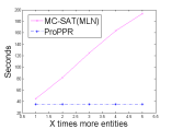
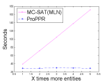
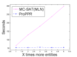
Figure 3: Run-time for non-recursive KB inference on NELL 10K subsets the using ProPPR (with a single thread) as a function of increasing the total entities by X times in the database. Total test queries are fixed in each subdomain. Left, the Google 10K dataset; middle, the Beatles 10K dataset; right, the Baseball 10K dataset.

Next we quantitatively compare ProPPR’s inference time, learning time, and performance with MLN, using the Alchemy toolkit. We use a KB with $M=1000$ entities, and test with a KB with $M=10,000$. The number of non-recursive KB rules is 95, 10, and 56 respectively, and the corresponding number of non-recursive/recursive PRA rules are 230, 29, and 148. The number of training queries are 466, 520, and 130, and the number of testing queries are 3143, 2552, and 4906. We set $\epsilon=0.01$ and $\alpha=0.1$. Again, we only take the top-1 PRA paths to construct ProPPR programs in this subsection.

In the first experiment, we investigate whether inference in ProPPR is sensitive to the size of graph. Using MLNs and ProPPR non-recursive KB programs trained on the 1K training subsets, we measure evaluate the inference time on the 10K testing subsets by varying the amount of entities in the database used at evaluation time. (Specifically, we use a fixed number of test queries, and increase the total number of entities in the KB by a factor of $X$, for various values of $X$.) In Figure. 3, we see that ProPPR’s runtime is independent of the size of the KB. In contrast, when comparing to MC-SAT, the default (and most efficient) inference method in MLN, we observe that inference time slows significantly when the database size grows.

In the second experiment, we compare ProPPR’s SGD training method with MLNs most efficient discriminative learning methods (voted perceptron and conjugate gradient) (Lowd and Domingos, 2007). To do this, we fixed the number of iterations of discriminative training in MLN to 10, and also fixed the number of SGD passes in ProPPR to 10. In Table 8, we show the runtime of various approaches on the three NELL subdomains. When running on the non-recursive KB theory, ProPPR has averages 1-2 seconds runtime across all domains, whereas training MLNs takes hours. When training on the non-recursive/recursive PRA theory, ProPPR is still efficient.

Table 8: Comparing the learning algorithm’s runtime between ProPPR and MLNs on the NELL 1K subsets .

Method	Google	Beatles	Baseball
ProPPR SGD KB non-recursive	2.6	2.3	1.5
MLN Conjugate Gradident	8604.3	1177.4	5172.9
MLN Voted Perceptron	8581.4	967.3	4194.5
ProPPR SGD PRA non-recursive	2.6	3.4	1.7
ProPPR SGD PRA recursive	4.7	3.5	2.1

We now examine the accuracy of ProPPR, in particular, the recursive formulation, and compare with MLN’s popular discriminative learning methods: voted perceptron and conjugate gradient. Here, we use AUC of the ROC curve as the measure. In Table 9, we see that MLNs outperform ProPPR’s using the non-recursive formulation. However, ProPPR’s recursive formulation outperforms all other methods, and shows the benefits of joint inference with recursive theories.

We should emphasize that the use of AUC means that we are evaluating only the ranking of the possible answers to a query; in other words, we are not measuring the quality of the actual probability scores produced by ProPPR, only the relative scores for a particular query. ProPPR’s random-walk scores tend to be very small for all potential answers, and are not well-suited to estimating probabilities in its current implementation.

Table 9: Comparing the learning algorithm’s AUC between recursive formulation of ProPPR and MLNs.

Methods	Google	Beatles	Baseball
ProPPR SGD KB non-recursive	0.568	0.510	0.652
MLN Conjugate Gradident	0.716	0.544	0.645
MLN Voted Perceptron	0.826	0.573	0.672
ProPPR SGD PRA non-recursive	0.894	0.922	0.930
ProPPR SGD PRA recursive	0.899	0.899	0.935

4.3 Varying The Size of The Theory

Table 10: AUCs for using top-k PRA paths for recursive formulation of ProPPR on NELL 100K and 1M datasets.

Methods	Google	Beatles	Baseball
ProPPR 100K top-1 recursive	0.950	0.884	0.952
ProPPR 100K top-2 recursive	0.954	0.916	0.950
ProPPR 100K top-3 recursive	0.959	0.953	0.952
ProPPR 1M top-1 recursive	0.955	0.955	0.955
ProPPR 1M top-2 recursive	0.961	0.960	0.960
ProPPR 1M top-3 recursive	0.964	0.964	0.964

So far, we have observed improved performance using the recursive theories of ProPPR, constructed from top $k=1$ PRA paths for each relation. Here we consider further increasing the size of the ProPPR program by including more PRA rules in the theory. In particular, we also extract the top-2 and top-3 PRA paths (limiting ourselves to rules with positive weights). On the 100K datasets, this increased the number of clauses in the recursive theories to 759, 624, and 765 in the Google, Beatles, and Baseball subdomains in the top-2 condition, and to 972, 806, and 983 in the top-3 condition. On the 1M datasets, we have now 801, 794, and 799 clauses in the top-2 case, and 1026, 1018, and 1024 in the top-3 setup. From Table 10, we observe that using more PRA paths improves performance on all three subdomains.

5 Experiments on Other tasks

As a further test of generality, we now present results using ProPPR on two other, smaller tasks. Our first sample task is an entity resolution task previously studied as a test case for MLNs (Singla and Domingos, 2006a). The program we use in the experiments is shown in Table 11: it is approximately the same as the MLN(B+T) approach from Singla and Domingos. To evaluate accuracy, we use the Cora dataset, a collection of 1295 bibliography citations that refer to 132 distinct papers. We set the regularization coefficient $\mu$ to $0.001$ and the number of epochs to 5.

Our second task is a bag-of-words classification task, which was previously studied as a test case for both ProbLog (Gutmann et al, 2010) and MLNs (Lowd and Domingos, 2007). In this experiment, we use the following ProPPR program:

class(X,Y) :-  has(X,W), isLabel(Y), related(W,Y).

related(W,Y) :-  true # w(W,Y).

which is a bag-of-words classifier that is approximately the same as the ones used in prior work (Gutmann et al, 2010; Lowd and Domingos, 2007). The dataset we use is the WebKb dataset, which includes a set of web pages from four computer science departments (Cornell, Wisconsin, Washington, and Texas). Each web page has one or multiple labels: course, department, faculty, person, research project, staff, and student. The task is to classify the given URL into the above categories. This dataset has a total of 4165 web pages. Using our ProPPR program, we learn a separate weight for each word for each label.

Table 11: ProPPR program used for entity resolution.

samebib(BC1,BC2) :-
author(BC1,A1),sameauthor(A1,A2),authorinverse(A2,BC2)	# author.
samebib(BC1,BC2) :-
title(BC1,A1),sametitle(A1,A2),titleinverse(A2,BC2)	# title.
samebib(BC1,BC2) :-
venue(BC1,A1),samevenue(A1,A2),venueinverse(A2,BC2)	# venue.
samebib(BC1,BC2) :-
samebib(BC1,BC3),samebib(BC3,BC2)	# tcbib.
sameauthor(A1,A2) :-
haswordauthor(A1,W),haswordauthorinverse(W,A2),keyauthorword(W)	# authorword.
sameauthor(A1,A2) :-
sameauthor(A1,A3),sameauthor(A3,A2)	# tcauthor.
sametitle(A1,A2) :-
haswordtitle(A1,W),haswordtitleinverse(W,A2),keytitleword(W)	# titleword.
sametitle(A1,A2) :-
sametitle(A1,A3),sametitle(A3,A2)	# tctitle.
samevenue(A1,A2) :-
haswordvenue(A1,W),haswordvenueinverse(W,A2),keyvenueword(W)	# venueword.
samevenue(A1,A2) :-
samevenue(A1,A3),samevenue(A3,A2)	# tcvenue.
keyauthorword(W) :- true	# authorWord(W).
keytitleword(W) :- true	# titleWord(W).
keyvenueword(W) :- true	# venueWord(W).

Table 12: Performance of the approximate PageRank-Nibble-Prove method on the Cora dataset, compared to the grounding by running personalized PageRank to convergence (power iteration). In all cases $\alpha=0.1$.

$\epsilon$	MAP	Time(sec)
0.0001	0.30	28
0.00005	0.40	39
0.00002	0.53	75
0.00001	0.54	116
0.000005	0.54	216
power iteration	0.54	819

For these smaller problems, we can also evaluate the cost of the PageRank-Nibble-Prove inference/grounding technique on Cora. Table 12 shows the time required for inference (with uniform weights) for a set of 52 randomly chosen entity-resolution tasks from the Cora dataset, using a Python implementation of the theorem-prover. We report the time in seconds for all 52 tasks, as well as the mean average precision (MAP) of the scoring for each query. It is clear that PageRank-Nibble-Prove offers a substantial speedup on these problems with little loss in accuracy: on these problems, the same level of accuracy is achieved in less than a tenth of the time.

  

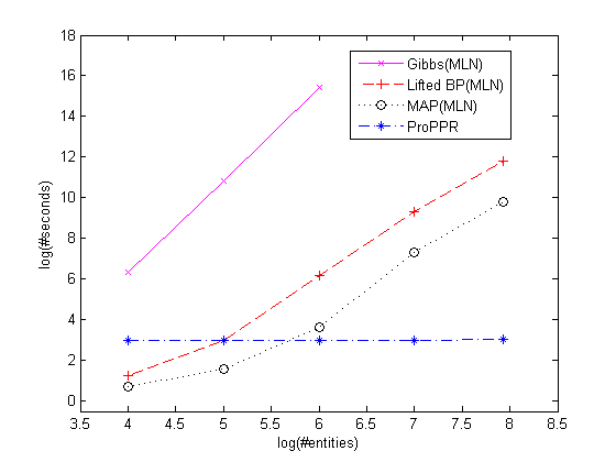
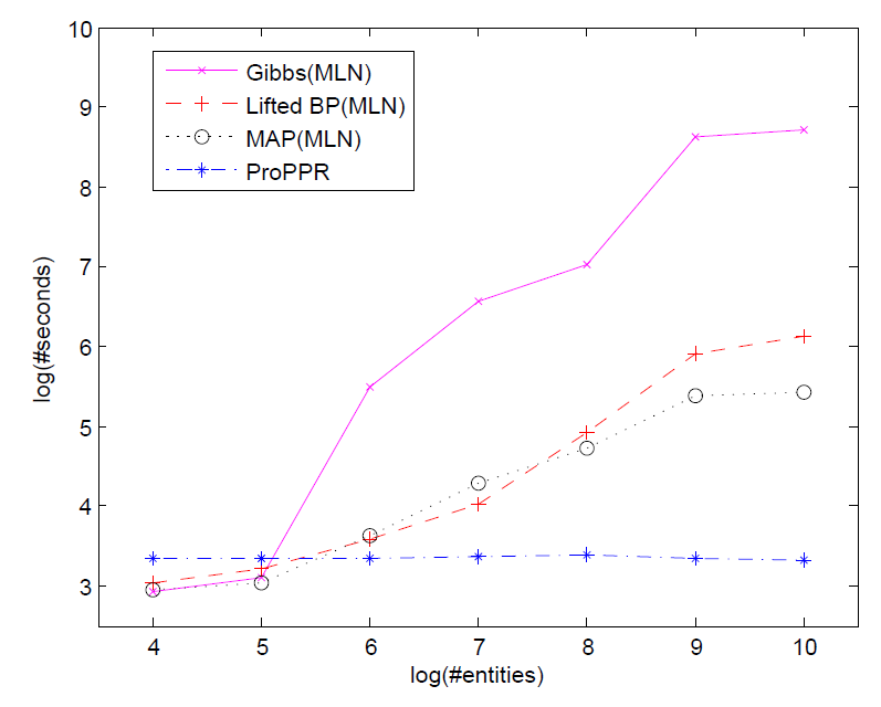
Figure 4: Run-time for inference on the using ProPPR (with a single thread) as a function of the number of entities in the database. The base of the log is 2. Left, the Cora dataset; right, the WebKB dataset.

While the speedup in inference time is desirable, the more important advantages of the local grounding approach are that (1) grounding time, and hence inference, need not grow with the database size and (2) learning can be performed in parallel, by using multiple threads for parallel computations of gradients in SGD. Figure 4 illustrates the first of these points: the scalability of the PageRank-Nibble-Prove method as database size increases. For comparison, we also show the inference time for MLNs with three inference methods: Gibbs refers to Gibbs sampling, Lifted BP is the lifted belief propagation method, and MAP is the maximum a posteriori inference approach. In each case the performance task is inference over 16 test queries.

Note that ProPPR’s runtime is constant, independent of the database size: it takes essentially the same time for $2^{8}=256$ entities as for $2^{4}=16$. In contrast, lifted belief propagation is up to 1000 times slower on the larger database.

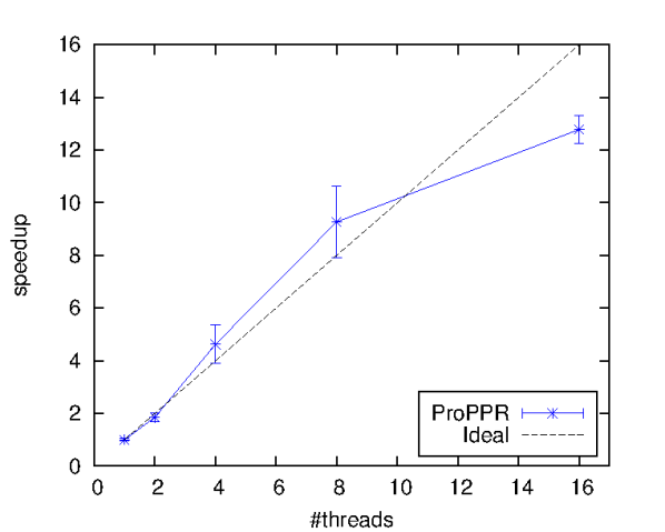
	Co.	Wi.	Wa.	Te.	Avg.
1	1190.4	504.0	1085.9	1036.4	954.2
2	594.9	274.5	565.7	572.5	501.9
4	380.6	141.8	404.2	396.6	330.8
8	249.4	94.5	170.2	231.5	186.4
16	137.8	69.6	129.6	141.4	119.6

Figure 5: Performance of the parallel SGD method. The $x$ axis is the number of threads on a multicore machine, and the $y$ axis is the speedup factor over a single-threaded implementation. Left, the Cora dataset; right, the WebKB dataset.

Figure 5 explores the speedup in learning (from grounded examples) due to multi-threading. The weight-learning is using a Java implementation of the algorithm which runs over ground graphs. For Cora, the speedup is nearly optimal, even with 16 threads running concurrently. For WebKB, while learning time averages about 950 seconds with a single thread, but this can be reduced to only two minutes if 16 threads are used. For comparison, Lowd and Domingos report that around 10,000 seconds were needed to obtain the best results were obtained for MLNs.

Table 13: AUC results on Cora citation-matching.

	Cites	Authors	Venues	Titles
MLN(Fig 1)	0.513	0.532	0.602	0.544
MLN(S&D)	0.520	0.573	0.627	0.629
ProPPR(w=1)	0.680	0.836	0.860	0.908
ProPPR	0.800	0.840	0.869	0.900

Table 14: AUC results on the WebKb classification task. ProbLog results are from (Gutmann et al, 2010), and MLN results are from (Lowd and Domingos, 2007). Co.: Cornell. Wi.: Wisconsin. Wa.: Washington. Te.: Texas.

	Co.	Wi.	Wa.	Te.	Avg.
ProbLog	–	–	–	–	0.606
MLN (VP)	–	–	–	–	0.605
MLN (CD)	–	–	–	–	0.604
MLN (CG)	–	–	–	–	0.730
ProPPR(w=1)	0.501	0.495	0.501	0.505	0.500
ProPPR	0.785	0.779	0.795	0.828	0.797

We finally consider the effectiveness of weight learning. For Cora, we train on the first four sections of the Cora dataset, and report results on the fifth. Following Singla and Domingos (Singla and Domingos, 2006a) we report performance as area under the ROC curve (AUC). Table 14 shows AUC on the test set used by Singla and Domingos for several methods. The line for MLN(Fig 1) shows results obtained by an MLN version of the program of Figure 1. The line MLN(S&D) shows analogous results for the best-performing MLN from (Singla and Domingos, 2006a). Compared to these methods, ProPPR does quite well even before training (with unit feature weights, w=1); the improvement here is likely due to the ProPPR’s bias towards short proofs, and the tendency of the PPR method to put more weight on shared words that are rare (and hence have lower fanout in the graph walk.) Training ProPPR improves performance on three of the four tasks, and gives the most improvement on citation-matching, the most complex task.

The results in Table 14 all use the same data and evaluation procedure, and the MLNs were trained with the state-of-the-art Alchemy system using the recommended commands for this data (which is distributed with Alchemy). However, we should note that the MLN results reproduced here are not identical to previous-reported ones (Singla and Domingos, 2006a). Singla and Domingos used a number of complex heuristics that are difficult to reproduce—e.g., one of these was combining MLNs with a heuristic, TFIDF-based matching procedure based on canopies (McCallum et al, 2000). While the trained ProPPR model outperformed the reproduced MLN model in all prediction tasks, it outperforms the reported results from Singla and Domingos only on venue, and does less well than the reported results on citation and author.

On the Webkb dataset, we use the usual cross-validation method (Lowd and Domingos, 2007; Gutmann et al, 2010): in each fold, for the four universities, we train on the three, and report result on the fourth. In Table 14, we show the detailed AUC results of each fold, as well as the averaged results. If we do not perform weight learning, the averaged result is equivalent to a random baseline. As reported by Gutmann et al. the ProbLog approach obtains an AUC of 0.606 on the dataset (Gutmann et al, 2010), and as reported by Lowd and Domingos, the results for voted perceptron algorithm (MLN VP, AUC $\approx 0.605$) and the contrastive divergence algorithm (MLN CD, AUC $\approx 0.604$) are in same range as ProbLog (Lowd and Domingos, 2007). ProPPR obtains an AUC of 0.797, which outperforms the prior results reported by ProbLog and MLN.

6 Related work

Although we have chosen here to compare mainly to MLNs (Richardson and Domingos, 2006; Singla and Domingos, 2006a), ProPPR represents a rather different philosophy toward language design: rather than beginning with a highly-expressive but intractable logical core, we begin with a limited logical inference scheme and add to it a minimal set of extensions that allow probabilistic reasoning, while maintaining stable, efficient inference and learning. While ProPPR is less expressive than MLNs (for instance, it is limited to definite clause theories) it is also much more efficient. This philosophy is similar to that illustrated by probabilistic similarity logic (PSL) (Brocheler et al, 2010); however, unlike ProPPR, PSL does not include a “local” grounding procedure, which leads to small inference problems, even for large databases. Our work also aligns with the lifted personalized PageRank (Ahmadi et al, 2011) algorithm, which can be easily incorporated as an alternative inference algorithm in our language.

Technically, ProPPR is most similar to stochastic logic programs (SLPs) (Cussens, 2001). The key innovation is the integration of a restart into the random-walk process, which, as we have seen, leads to very different computational properties.

ProbLog (De Raedt et al, 2007), like ProPPR, also supports approximate inference, in a number of different variants. An extension to ProbLog also exists which uses decision theoretic analysis to determine when approximations are acceptable (Van den Broeck et al, 2010). Although this paper does present a very limited comparison with ProbLog on the WebKB problem (in Table 14o) a further comparison of speed and utility of these different approaches to approximate inference is an important topic for future work.

There has also been some prior work on reducing the cost of grounding probabilistic logics: notably, Shavlik et al (Shavlik and Natarajan, 2009) describe a preprocessing algorithm called FROG that uses various heuristics to greatly reduce grounding size and inference cost, and Niu et al (Niu et al, 2011a) describe a more efficient bottom-up grounding procedure that uses an RDBMS. Other methods that reduce grounding cost and memory usage include “lifted” inference methods (e.g., (Singla and Domingos, 2008)) and “lazy” inference methods (e.g., (Singla and Domingos, 2006b)); in fact, the LazySAT inference scheme for Markov networks is broadly similar algorithmically to PageRank-Nibble-Prove, in that it incrementally extends a network in the course of theorem-proving. However, there is no theoretical analysis of the complexity of these methods, and experiments with FROG and LazySAT suggest that they still lead to a groundings that grow with DB size, albeit more slowly.

As noted above, ProPPR is also closely related to the PRA, learning algorithm for link prediction (Lao and Cohen, 2010), like ProPPR, PRA uses random walk processes to define a distribution, rather than some other forms of logical inference, such as belief propagation. In this respect PRA and ProPPR appear to be unique among probabilistic learning methods; however, this distinction may not be as great as it first appears, as it is known there are close connections between personalized PageRank and traditional probabilistic inference schemes. PRA, however, is much more limited than ProPPR, again, as noted above. However, unlike PRA, we do not consider the task of searching for logic program clauses.

7 Conclusions

We described a new probabilistic first-order language which is designed with the goal of highly efficient inference and rapid learning. ProPPR takes Prolog’s SLD theorem-proving, extends it with a probabilistic proof procedure, and then limits this procedure further, by including a “restart” step which biases the system to short proofs. This means that ProPPR has a simple polynomial-time proof procedure, based on the well-studied personalized PageRank (PPR) method.

Following prior work on approximate PPR algorithms, we designed a local grounding procedure for ProPPR, based on local partitioning methods (Andersen et al, 2006, 2008), which leads to an inference scheme that is an order of magnitude faster that the conventional power-iteration approach to computing PPR, takes time $O(\frac{1}{\epsilon\alpha^{\prime}})$, independent of database size. This ability to “locally ground” a query also makes it possible to partition the weight learning task into many separate gradient computations, one for each training example, leading to a weight-learning method that can be easily parallelized. In our current implementation, an additional order-of-magnitude speedup in learning is made possible by parallelization. Experimentally, we showed that ProPPR performs well on an entity resolution task, and a classification task. It also performs well on a difficult problem involving joint inference over an automatically-constructed KB, an approach that leads to improvements over learning each predicate separately. Most importantly, ProPPR scales well, taking only a few seconds on a conventional desktop machine to learn weights for a mutually recursive program with hundreds of clauses, which define scores of interrelated predicates, over a substantial KB containing one million entities.

In future work, we plan to explore additional applications of, and improvements to, ProPPR. One improvement would be to extend ProPPR to include “hard” logical predicates, an extension whose semantics have been fully developed for SLPs (Cussens, 2001). Also, in the current learning process, the grounding for each query actually depends on the ProPPR model parameters. We can potentially get improvement by making the process of grounding more closely coupled with the process of parameter learning. Finally, we note that further speedups in multi-threading might be obtained by incorporating newly developed approaches to loosely synchronizing parameter updates for parallel machine learning methods (Ho et al, 2013).

Acknowledgements

This work was sponsored in part by DARPA grant FA87501220342 to CMU and a Google Research Award.

References

- Ahmadi et al (2011) Ahmadi B, Kersting K, Sanner S (2011) Multi-evidence lifted message passing, with application to pagerank and the kalman filter. In: Proceedings of the Twenty-Second international joint conference on Artificial Intelligence
- Andersen et al (2006) Andersen R, Chung FRK, Lang KJ (2006) Local graph partitioning using pagerank vectors. In: FOCS, pp 475–486
- Andersen et al (2008) Andersen R, Chung FRK, Lang KJ (2008) Local partitioning for directed graphs using pagerank. Internet Mathematics 5(1):3–22
- Backstrom and Leskovec (2011) Backstrom L, Leskovec J (2011) Supervised random walks: predicting and recommending links in social networks. In: Proceedings of the fourth ACM international conference on Web search and data mining
- Brocheler et al (2010) Brocheler M, Mihalkova L, Getoor L (2010) Probabilistic similarity logic. In: Proceedings of the Conference on Uncertainty in Artificial Intelligence
- Van den Broeck et al (2010) Van den Broeck G, Thon I, van Otterlo M, De Raedt L (2010) Dtproblog: A decision-theoretic probabilistic prolog. In: AAAI
- Carlson et al (2010) Carlson A, Betteridge J, Kisiel B, Settles B, Jr ERH, Mitchell TM (2010) Toward an architecture for never-ending language learning. In: Fox M, Poole D (eds) AAAI, AAAI Press
- Chakrabarti (2007) Chakrabarti S (2007) Dynamic personalized PageRank in entity-relation graphs. In: Proceedings of the 16th international conference on World Wide Web
- Cohen (2000) Cohen WW (2000) Data integration using similarity joins and a word-based information representation language. ACM Transactions on Information Systems 18(3):288–321
- Cohen (2010) Cohen WW (2010) Graph Walks and Graphical Models. Carnegie Mellon University, School of Computer Science, Machine Learning Department
- Cussens (2001) Cussens J (2001) Parameter estimation in stochastic logic programs. Machine Learning 44(3):245–271
- De Raedt et al (2007) De Raedt L, Kimmig A, Toivonen H (2007) Problog: A probabilistic prolog and its application in link discovery. In: Proceedings of the 20th international joint conference on Artifical intelligence
- Fuhr (1995) Fuhr N (1995) Probabilistic datalog—a logic for powerful retrieval methods. In: Proceedings of the 18th annual international ACM SIGIR conference on Research and development in information retrieval, ACM, pp 282–290
- Gutmann et al (2010) Gutmann B, Kimmig A, Kersting K, De Raedt L (2010) Parameter estimation in problog from annotated queries. CW Reports
- Ho et al (2013) Ho Q, Cipar J, Cui H, Lee S, Kim JK, Gibbons PB, Gibson GA, Ganger G, Xing E (2013) More effective distributed ml via a stale synchronous parallel parameter server. In: Advances in Neural Information Processing Systems, pp 1223–1231
- Hoffmann et al (2011) Hoffmann R, Zhang C, Ling X, Zettlemoyer LS, Weld DS (2011) Knowledge-based weak supervision for information extraction of overlapping relations. In: ACL, pp 541–550
- Jha and Suciu (2012) Jha A, Suciu D (2012) Probabilistic databases with markoviews. Proceedings of the VLDB Endowment 5(11):1160–1171
- Lao and Cohen (2010) Lao N, Cohen WW (2010) Relational retrieval using a combination of path-constrained random walks. Machine Learning 81(1):53–67
- Lao et al (2011) Lao N, Mitchell TM, Cohen WW (2011) Random walk inference and learning in a large scale knowledge base. In: EMNLP, ACL, pp 529–539
- Lloyd (1987) Lloyd JW (1987) Foundations of Logic Programming: Second Edition. Springer-Verlag
- Lowd and Domingos (2007) Lowd D, Domingos P (2007) Efficient weight learning for markov logic networks. In: Knowledge Discovery in Databases: PKDD 2007, Springer, pp 200–211
- McCallum et al (2000) McCallum A, Nigam K, Ungar LH (2000) Efficient clustering of high-dimensional data sets with application to reference matching. In: Knowledge Discovery and Data Mining, pp 169–178, URL citeseer.nj.nec.com/article/mccallum00efficient.html
- Niu et al (2011a) Niu F, Ré C, Doan A, Shavlik J (2011a) Tuffy: Scaling up statistical inference in markov logic networks using an RDBMS. Proceedings of the VLDB Endowment 4(6):373–384
- Niu et al (2011b) Niu F, Recht B, Ré C, Wright SJ (2011b) Hogwild!: A lock-free approach to parallelizing stochastic gradient descent. arXiv preprint arXiv:11065730
- Page et al (1998) Page L, Brin S, Motwani R, Winograd T (1998) The PageRank citation ranking: Bringing order to the web. In: Technical Report, Computer Science department, Stanford University
- Poon and Domingos (2007) Poon H, Domingos P (2007) Joint inference in information extraction. In: Proceedings of the National Conference on Artificial Intelligence
- Poon and Domingos (2008) Poon H, Domingos P (2008) Joint unsupervised coreference resolution with markov logic. In: Proceedings of the Conference on Empirical Methods in Natural Language Processing, Association for Computational Linguistics, pp 650–659
- Richardson and Domingos (2006) Richardson M, Domingos P (2006) Markov logic networks. Mach Learn 62(1-2):107–136, DOI http://dx.doi.org/10.1007/s10994-006-5833-1
- Shavlik and Natarajan (2009) Shavlik J, Natarajan S (2009) Speeding up inference in markov logic networks by preprocessing to reduce the size of the resulting grounded network. In: Proceedings of the Twenty-first International Joint Conference on Artificial Intelligence (IJCAI-09)
- Singhal (2012) Singhal A (2012) Introducing the knowledge graph: things, not strings. the official Google blog: http://googleblogblogspotcom/2012/05/ introducing-knowledge-graph-things-nothtml
- Singla and Domingos (2006a) Singla P, Domingos P (2006a) Entity resolution with markov logic. In: Data Mining, 2006. ICDM’06. Sixth International Conference on
- Singla and Domingos (2006b) Singla P, Domingos P (2006b) Memory-efficient inference in relational domains. In: Proceedings of the national conference on Artificial intelligence
- Singla and Domingos (2008) Singla P, Domingos P (2008) Lifted first-order belief propagation. In: Proceedings of the 23rd national conference on Artificial intelligence
- Suchanek et al (2007) Suchanek FM, Kasneci G, Weikum G (2007) Yago: a core of semantic knowledge. In: Proceedings of the 16th international conference on World Wide Web, ACM, pp 697–706
- Tong et al (2006) Tong H, Faloutsos C, Pan JY (2006) Fast random walk with restart and its applications. In: ICDM, IEEE Computer Society, pp 613–622
- Zinkevich et al (2009) Zinkevich M, Smola A, Langford J (2009) Slow learners are fast. Advances in Neural Information Processing Systems 22:2331–2339
- Zinkevich et al (2010) Zinkevich M, Weimer M, Smola A, Li L (2010) Parallelized stochastic gradient descent. Advances in Neural Information Processing Systems