Large deviation estimates
involving deformed exponential functions

Abstract

We study large deviation properties of probability distributions with either a compact support or a fat tail by comparing them with q-deformed exponential distributions. Our main result is a large deviation property for probability distributions with a fat tail.

1 Introduction

The Law of Large Numbers (LLN) states that the arithmetic mean of i.i.d. variables $X_{1},X_{2},\cdots,X_{n}$ converges to the first moment ${\mathbb{E}}X_{k}$ of the probability distribution. The Large Deviation Principle (LDP) is the property that the probability that the arithmetic mean has a deviating value is exponentially small in the number of variables $n$. It is an important assumption for the theorem of Varadhan [1], which deals with the asymptotic evaluation of certain integrals. See also [2, 3, 4, 5, 6, 7].

Varadhan’s theorem is a generalization of Laplace’s method of evaluating integrals. As such it is highly relevant for the axiomatic formulation of statistical mechanics. The standard reference in this direction is the book of Ellis [2]. A more recent review is found in [7]. The breakdown of Varadhan’s theorem is related with the occurrence of phase transitions in models of statistical physics. It is due to the appearance of strong correlations between the variables $X_{k}$. Another reason of failure of Varadhan’s theorem can be that the LDP is not satisfied. This is the case for instance when the probability distribution of the variables $X_{k}$ has a fat tail. It is the latter situation which is considered in the present work.

Mathematicians have studied large deviations in the context of probability distributions with a fat tail starting with the works of Heyde [8, 9] and Nagaev [10, 11]. See also [12, 13, 14, 15, 16, 17, 18, 19]. The present work starts from the question whether a systematic use of so-called q-deformed exponential functions can make a contribution to this area of research. The q-deformed exponential functions, used in the present work, have been introduced [20] in the context of non-extensive statistical physics [21]. See also [22, 23]. Our approach differs from that of [24] and of [25] who consider strong correlations in the context of nonextensive statistical mechanics.

The strategy of the paper is to mimic the standard approach, replacing where meaningful the exponential function by a deformed function. We therefore start in the next section by reviewing some standard inequalities. Section 3 gives the definition of q-deformed exponential and logarithmic functions. Section 4 deals with an application of the Markov inequality in the case of distributions with a compact support. The treatment of distributions with a fat tail is more difficult. Before discussing them in Section 6 we first study the q-exponential distributions in Section 5. The final Section 7 contains a summary and an evaluation of what has been obtained.

2 The standard inequality

The Markov inequality

$${\rm Prob\,}\left(X\geq x\right)\leq\frac{{\mathbb{E}}X}{x},\quad x>0,$$ (1)

valid for any random variable $X$ assuming non-negative values, implies that for any random variable $X$ which assumes real values one has

$${\rm Prob\,}\left(X\geq x\right)\leq A(a)e^{-ax},\quad a\geq 0.$$ (2)

This expression involves the moment generating function

$$A(a)={\mathbb{E}}e^{aX}.$$ (3)

Its existence is called Cramér’s condition. For a sequence $X_{1},X_{2},\cdots,X_{n}$ of i.i.d. variables there follows

$${\rm Prob\,}\left(\frac{1}{n}\sum_{k=1}^{n}X_{k}\geq x\right)\leq A^{n}(a)e^{-nax}.$$ (4)

Introduce a rate function $I(x)$ defined by

$$I(x)=\sup_{\theta\geq 0}\{\theta x-\ln A(\theta)\}\leq+\infty.$$ (5)

Note that we change notations from $a$ to $\theta$ for compatibility with expressions later on. The function $I(x)$ is convex non-decreasing, with $I(0)=0$ and $\lim_{x\rightarrow+\infty}I(x)=+\infty$ (we assume that $A(a)$ is finite for some $a>0$).

One obtains

$${\rm Prob\,}\left(\frac{1}{n}\sum_{k=1}^{n}X_{k}\geq x\right)\leq e^{-nI(x)}.$$ (6)

When $I(x)$ is strictly positive then an outcome larger than $x$ is a large deviation and its probability decays exponentially fast in $n$.

3 Deformed logarithmic and exponential functions

Fix $q$ satisfying $0<q<2$, $q\not=1$. The $q$-deformed logarithm is defined by [20, 23]

$$\ln_{q}(u)=\frac{1}{1-q}\left(u^{1-q}-1\right)\quad u>0.$$ (7)

In the limit $q=1$ it reduces to the natural logarithm $\ln u$. The inverse function is the $q$-deformed exponential. It is defined on the whole of the real axis by

$$\exp_{q}(u)=\left[1+(1-q)u\right]_{+}^{1/(1-q)}\leq+\infty.$$ (8)

Here, $[u]_{+}$ denotes the positive part of $u$. Note that $\exp_{q}(\ln_{q}(u))=u$ holds for all $u>0$. However, $\ln_{q}(\exp_{q}(u))$ may differ from $u$ when $\exp_{q}(u)$ diverges or vanishes.

For further use we mention that

$$\exp_{q}(u)\exp_{2-q}(-u) = \left(\frac{\left[1+(1-q)u\right]_{+}}{\left[1+(1-q)u\right]_{+}}\right)^{1/(1-q)}$$ (9)

$$= 1,$$ (10)

whenever $1+(1-q)u>0$.

The following two properties are used later on.

Proposition 3.1

The function $\exp_{q}(x)$ is log-concave when $q<1$ and log-convex when $q>1$.

Proof

Let $f(x)=\ln\exp_{q}(x)$. Its first derivative equals

$$f^{\prime}(x) = \left[\exp_{q}(x)\right]^{q-1}$$ (11)

$$= \frac{1}{\left[1+(1-q)x\right]_{+}}.$$ (12)

This function is decreasing when $q<1$ and increasing when $q>1$.

$\square$

Proposition 3.2

Let $0<q<1$ and let $q^{*}=2-q$. Then one has for all $a>0$ and $b>0$ that

$$\exp_{q}(a+b)\leq\exp_{q}(a)\exp_{q}(b)$$ (13)

and

$$\exp_{q^{*}}(-a-b)\geq\exp_{q^{*}}(-a)\exp_{q^{*}}(-b).$$ (14)

The proof is straightforward. Note that equalities hold in the case $q=q^{*}=1$.

The $q$-deformed exponential distribution is defined on the positive axis and has $\exp_{q}(-ax)$ as its tail distribution. Hence the probability density is

$$f_{q}(x) = a\left(\exp_{q}(-ax)\right)^{q},\quad x\geq 0,$$ (15)

$$= a\left[1-(1-q)ax\right]_{+}^{q/(1-q)}.$$ (16)

When $0<q<1$ then the distribution has a compact support, namely

$$\left[0,\frac{1}{a(1-q)}\right].$$ (17)

On the other hand, when $1<q<2$ then it has a fat tail

$$f_{q}(x)\sim\frac{1}{[(q-1)ax]^{q/(q-1)}}.$$ (18)

These two cases are rather different. Therefore we will treat them separately. However, in order to avoid confusion we restrict in what follows the values of the parameter $q$ to the interval $[0,1]$ and use $q^{*}$ to denote values in the range between 1 and 2. In fact, this convention has been followed already in the previous proposition.

4 The case of a compact support

4.1 A deformed inequality

The Markov inequality implies the following analogue of (4).

Proposition 4.1

Let be given i.i.d. random variables $X_{1},X_{2},\cdots,X_{n}$. One has for all $x$ and for all $a>0$ for which $(1-q)ax<1$

$${\rm Prob\,}\left(\frac{1}{n}\sum_{k=1}^{n}X_{k}\geq x\right)\leq\left[\exp_{q}(-ax)\right]^{n}A^{n}(a),$$ (19)

with

$$A(a)={\mathbb{E}}\exp_{q^{*}}(aX_{1}).$$ (20)

Proof

Because $\exp_{q^{*}}$ is log-convex one has

$$\ln\exp_{q^{*}}\left(\frac{1}{n}\sum_{k=1}^{n}aX_{k}\right)\leq\frac{1}{n}\sum_{k=1}^{n}\ln\exp_{q^{*}}\left(aX_{k}\right).$$ (21)

This can be written as

$${\mathbb{I}}_{\sum_{k=1}^{n}X_{k}\geq nx}\,\left[\exp_{q^{*}}\left(ax\right)\right]^{n} \leq \left[\exp_{q^{*}}\left(\frac{1}{n}\sum_{k=1}^{n}aX_{k}\right)\right]^{n}$$ (22)

$$\leq \prod_{k=1}^{n}\exp_{q^{*}}\left(aX_{k}\right).$$ (23)

Here, ${\mathbb{I}}_{c}$ denotes the indicator function which equals 1 when $c$ is satisfied and vanishes otherwise. Take the expectation. This gives

$${\rm Prob\,}\left(\frac{1}{n}\sum_{k=1}^{n}X_{k}\geq x\right)\left[\exp_{q^{*}}\left(ax\right)\right]^{n}\leq A^{n}(a).$$ (24)

The latter can be written as (19).

$\square$

We will see in an example later on that as a bound the above result is less sharp than (4).

4.2 Legendre structure

Introduce now a parameter $\theta$ defined by

$$\theta=\left[{\mathbb{E}}\exp_{q^{*}}(aX_{1})\right]^{1-q}a.$$ (25)

Lemma 4.2

$\theta$ is a strictly increasing function of $a$ on the open interval of $a$-values for which $0<{\mathbb{E}}\exp_{q^{*}}(aX_{1})<+\infty$.

Proof

One calculates

$$\frac{{\rm d}\theta}{{\rm d}a} = \left[{\mathbb{E}}\exp_{q^{*}}(aX_{1})\right]^{1-q}$$ (27)

$$+(1-q)\left[{\mathbb{E}}\exp_{q^{*}}(aX_{1})\right]^{-q}{\mathbb{E}}\left(\left[\exp_{q^{*}}(aX_{1})\right]^{q^{*}}X_{1}\right)a$$

$$= \left[{\mathbb{E}}\exp_{q^{*}}(aX_{1})\right]^{-q}{\mathbb{E}}\left[\exp_{q^{*}}(aX_{1})\right]^{q^{*}}$$ (28)

$$> 0.$$ (29)

$\square$

A consequence of this lemma is that the functional dependence $\theta(a)$ may be inverted to $a(\theta)$. Hence we can define a function $\Phi(\theta)$ by

$$\Phi(\theta)=\ln_{q}{\mathbb{E}}\exp_{q^{*}}(aX_{1}).$$ (30)

Note that $a\downarrow 0$ implies $\theta=0$. Let

$${\overline{\theta}} = \sup_{a>0}\theta(a)\leq+\infty.$$ (31)

Then $\Phi(\theta)$ is defined for $0<\theta<\overline{\theta}$.

4.3 A Theorem

The Proposition 4.1 can now be reformulated as follows.

Theorem 4.3

Let be given i.i.d. random variables $X_{1},X_{2},\cdots,X_{n}$. Fix $q$ such that $0<q<1$ and let $q^{*}=2-q$. Assume that ${\mathbb{E}}\exp_{q^{*}}(aX_{1})$ is finite for small positive $a$. Then one has for all $x$ that

$${\rm Prob\,}\left(\frac{1}{n}\sum_{k=1}^{n}X_{k}\geq x\right)\leq\left[\exp_{q}(-I(x))\right]^{n},$$ (32)

with the rate function $I(x)$ given by

$$I(x)=\sup_{0<\theta<\overline{\theta}}\{\theta x-\Phi(\theta)\}.$$ (33)

The function $\Phi(\theta)$ is defined by (30). The range $(0,\overline{\theta})$ is defined by (31).

Proof

A short calculation shows that the r.h.s. of (19) can be written as

$$\left[\exp_{q}(\Phi(\theta)-\theta x)\right]^{n}.$$ (34)

In this expression $\theta$ has an arbitrary value in $(0,\overline{\theta})$. The proof then follows by taking the infimum over $\theta$.

$\square$

4.4 Example: the uniform distribution

Consider for instance a random variable $X$ uniformly distributed on the interval $[0,1]$. A short calculation gives

$$A(a) \equiv {\mathbb{E}}\exp_{q^{*}}(aX)$$ (35)

$$= \frac{1}{qa}\left[\left\{\exp_{q^{*}}(a)\right\}^{q}-1\right].$$ (36)

This yields

$$\theta=aA^{1-q}=a\left[\frac{\{\exp_{q^{*}}(a)\}^{q}-1}{qa}\right]^{1-q}$$ (37)

and

$$\Phi(\theta) = \ln_{q}A$$ (38)

$$= \frac{1}{1-q}\left[\frac{\theta}{a}-1\right].$$ (39)

A short calculation shows that the quantity $\Phi-\theta x$ is minimal when $a=0$ or $a$ is a solution of

$$\exp_{q^{*}}(a)=1+\frac{a}{1-a+axq}.$$ (40)

A series expansion for small values of $a$ yields

$$\Phi(a)-\theta x=\left(\frac{1}{2}-x\right)a+{\rm O}(a^{2}).$$ (41)

This shows that $I(x)\not=0$ whenever $x>1/2$. Hence, in this case (40) has a useful solution. Note that $a<1/(1-q)$ is needed to keep $\exp_{q^{*}}(a)$ finite.

Take for instance $q=1/2$. This gives $A=2/(2-a)$, $\theta=a\sqrt{A}$ and $\Phi=2(\theta/a-1)$. The minimum is obtained for $a=0$ or $a=4(x-1/2)/x$. The latter requires $1/2<x<1$. One obtains

$$I(x) = 2-4\sqrt{x(1-x)},\quad\frac{1}{2}<x<1$$ (42)

The final result is then

$${\rm Prob\,}\left(\frac{1}{n}\sum_{k=1}^{n}X_{k}\geq x\right)\leq\left[4x(1-x)\right]^{n},\quad\frac{1}{2}\leq x\leq 1.$$ (43)

Note that this result can be written as

$${\rm Prob\,}\left(\frac{1}{n}\sum_{k=1}^{n}X_{k}\geq x\right)\leq e^{-nI_{1}(x)},\quad\frac{1}{2}\leq x\leq 1$$ (44)

with

$$I_{1}(x)=\ln 2x+\ln 2(1-x).$$ (45)

One can show numerically that the bound (43) is less sharp than the one obtained by the standard inequality ($q=1$). However, (43) has the advantage of being expressed in a closed form. See the Figure 1.

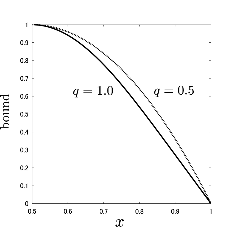
Figure 1: Upper bounds for the probability that $X_{1}$ is larger than $x$ given the uniform distribution on the interval $[0,1]$. From top to bottom the curves correspond with $q=1/2$ and $q=1$ (standard case).

5 The $q^{*}$-deformed exponential distribution

5.1 Definition

Fix $q$ between 0 and 1, as before, and let $q^{*}=2-q$. Let

$$\eta(x) = \exp_{q^{*}}(-x)\quad x\geq 0,$$ (46)

$$= 1\quad x\leq 0.$$ (47)

Let $X$ be a random variable distributed according to the distribution $f(x)$ given by

$$f(x) \equiv \frac{{\rm d}\,}{{\rm d}x}(1-\eta(x))$$ (48)

$$= \left[\exp_{q^{*}}(-x)\right]^{q^{*}}\quad\mbox{if }x>0,$$ (49)

$$= 0\qquad\qquad\mbox{if }x<0.$$ (50)

Then one has

$${\rm Prob\,}\left(X\geq x\right)=\eta(x).$$ (51)

This distribution is a special case of the Lomax distribution [26] and hence of a type-II Pareto distribution. Its first moment exists and is given by

$${\mathbb{E}}X=\frac{1}{q}.$$ (52)

An important property of this distribution is the following. Note that in the case of the exponential distribution (this is the $q=1$-limit) it holds with equality.

Proposition 5.1

$$\eta(a)\eta(b)\leq\eta(a+b),\quad\mbox{for all }a>0,b>0.$$ (53)

Proof

One can write

$$\eta(a)\eta(b) = \frac{1}{[1+(1-q)a]^{\frac{1}{1-q}}}\,\frac{1}{[1+(1-q)b]^{\frac{1}{1-q}}}$$ (54)

$$= \frac{1}{[1+(1-q)(a+b)+(1-q)^{2}ab]^{\frac{1}{1-q}}}$$ (55)

$$\leq \frac{1}{[1+(1-q)(a+b)]^{\frac{1}{1-q}}}$$ (56)

$$= \eta(a+b).$$ (57)

$\square$

5.2 Sums of i.i.d. variables

The law of large numbers holds for the distribution (50). Hence one can expect that some form of a large deviation principle should hold.

Consider a sequence of i.i.d. variables $X_{1}$, $X_{2}$, $\cdots$, $X_{n}$, all distributed according to $f(x)$ given by (50) and introduce tail distributions $\eta_{n}$ defined by

$$\eta_{n}(x)={\rm Prob\,}\left(\frac{1}{n}\sum_{k=1}^{n}X_{k}\geq x\right).$$ (58)

These functions will be used later on in the formulation of a large deviation estimate. They satisfy the inequalities

$$\left[\eta(x)\right]^{n}\leq\eta_{n}(x)\leq 1.$$ (59)

The lower bound can be improved easily. Indeed, one has

Proposition 5.2

For all $x>0$ is

$$1-[1-\eta(nx)]^{n}\leq\eta_{n}(x).$$ (60)

This result is a special case of Proposition 6.2 found below.

It turns out to be very difficult to obtain a sharp upper bound, valid for arbitrary values of $n$. Therefore we go immediately over to an asymptotic analysis.

5.3 Asymptotic analysis

For large values of $x$ the functions $\eta_{n}(x)$ satisfy the relation $\eta_{n}(x)\sim n\eta(nx)$. This property is known to be equivalent with sub-exponentiality [27]. From

$$\eta(x)\sim\left[\frac{1}{(1-q)x}\right]^{1/(1-q)}$$ (61)

then follows that

$$n^{q/(1-q)}\eta_{n}(x)\sim\eta(x)\quad\mbox{ as }x\rightarrow\infty.$$ (62)

This suggests that for large $n$ and for $x>{\mathbb{E}}X_{1}=1/q$ the expression
$n^{q/(1-q)}\eta_{n}(x)$ remains bounded when $n$ tends to infinity. This turns out to be correct, as discussed below.

From the lower bound (60) follows immediately that

$$\liminf_{n\rightarrow\infty}n^{q/(1-q)}\eta_{n}(x)\geq\left[\frac{1}{(1-q)x}\right]^{\frac{1}{1-q}},\quad x>0.$$ (63)

Indeed, one has

$$n^{q/(1-q)}\left(1-[1-\eta(nx)]^{n}\right) \sim n^{1+q/(1-q)}\eta(nx)$$ (64)

$$\sim n^{1+q/(1-q)}\left[\frac{1}{(1-q)nx}\right]^{1/(1-q)}$$

$$= \left[\frac{1}{(1-q)x}\right]^{1/(1-q)}.$$ (65)

In particular, this result implies that the standard Large Deviation Principle is not satisfied. For the asymptotic upper bound we have to appeal on the mathematical analysis originally started by Heyde [8, 9] and Nagaev [10, 11]. The $q$-exponential distribution belongs to the class of distributions they consider. As a consequence, one has the following result.

Proposition 5.3

For all $x>{\mathbb{E}}X_{1}$ and for $n$ tending to $\infty$ is

$$\eta_{n}(x)\sim n\eta(n(x-{\mathbb{E}}X_{1}))\sim\frac{1}{n^{\frac{q}{1-q}}}\left[\frac{1}{x-{\mathbb{E}}X_{1}}\right]^{\frac{1}{1-q}}.$$ (66)

Proof

See for instance Theorem A in [17].

$\square$

6 The case of a fat tail

6.1 The deformed inequality

The result of Proposition 4.1 is not valid for $q>1$ because the proof uses that $\exp_{q^{*}}$ is log-convex. However, a slightly different result is obtained using Proposition 3.2 instead of 3.1.

Proposition 6.1

Let be given positive i.i.d. random variables $X_{1},X_{2},\cdots,X_{n}$. One has for all $x>0$ and for all $a>0$

$${\rm Prob\,}\left(\frac{1}{n}\sum_{k=1}^{n}X_{k}\geq x\right)\leq\exp_{q^{*}}(-anx)A^{n}(a),$$ (67)

with

$$A(a)={\mathbb{E}}\exp_{q}(aX_{1}).$$ (68)

Proof

Because $a>0$ and $\exp_{q}$ is an increasing function one has

$${\mathbb{I}}_{\{\sum_{k=1}^{n}X_{k}\geq nx\}}\exp_{q}\left(anx\right) \leq \exp_{q}\left(a\sum_{k=1}^{n}X_{k}\right).$$ (69)

Now use Proposition 3.2 to obtain

$${\mathbb{I}}_{\{\sum_{k=1}^{n}X_{k}\geq nx\}}\exp_{q}\left(anx\right) \leq \prod_{k=1}^{n}\exp_{q}\left(aX_{k}\right).$$ (70)

Take the expectation. This gives, with the help of the i.i.d. property of the random variables,

$${\rm Prob\,}\left(\sum_{k=1}^{n}X_{k}\geq nx\right)\exp_{q}\left(anx\right) \leq \left[{\mathbb{E}}\exp_{q}\left(aX_{1}\right)\right]^{n}.$$ (71)

This result can be written as (67).

$\square$

We will use this result only for $n=1$. The factor $A^{n}(a)$ in the r.h.s. of (67) diverges exponentially fast and prohibits sharp estimates in the limit of large $n$.

6.2 Sums of i.i.d. variables

The lower bound (60) is a special case of the following easy lower bound.

Proposition 6.2

Let be given i.i.d. random variables $X,X_{1},X_{2},\cdots,X_{n}$, all following the same probability distribution $f(x)$. Let ${\overline{F}}(x)$ denote the corresponding tail distribution. Then one has

$$1-[1-{\overline{F}}(nx)]^{n}\leq{\rm Prob\,}\left(\frac{1}{n}\sum_{k=1}^{n}X_{k}\geq x\right).$$ (72)

Proof

One has

$${\rm Prob\,}\left(\frac{1}{n}\sum_{k=1}^{n}X_{k}\geq x\right) = \int{\rm d}x_{1}\,f(x_{1})\cdots\int{\rm d}x_{n}\,f(x_{n}){\mathbb{I}}_{\{\sum x_{k}\geq nx\}}$$ (74)

$$= n\int{\rm d}x_{1}\,f(x_{1})\int^{x_{1}}{\rm d}x_{2}\,f(x_{2})$$

$$\cdots\int^{x_{1}}{\rm d}x_{n}\,f(x_{n}){\mathbb{I}}_{\{\sum x_{k}\geq nx\}}.$$

To see this note that one may assume that one of the variables, say $x_{1}$, is larger than the others. Next use that it is sufficient that $x_{1}$ is larger than $nx$ to obtain

$${\rm Prob\,}\left(\frac{1}{n}\sum_{k=1}^{n}X_{k}\geq x\right) \geq n\int_{nx}{\rm d}x_{1}\,f(x_{1})\int^{x_{1}}{\rm d}x_{2}\,f(x_{2})\cdots\int^{x_{1}}{\rm d}x_{n}\,f(x_{n})$$ (75)

$$= n\int_{nx}{\rm d}x_{1}\,f(x_{1})\left[1-{\overline{F}}(x_{1})\right]^{n-1}$$ (76)

$$= 1-[1-{\overline{F}}(nx)]^{n}.$$ (77)

$\square$

The Proposition 6.1 is used to obtain an upper bound.

Proposition 6.3

Let be given i.i.d. random variables $X,X_{1},X_{2},\cdots,X_{n}$. Fix $q$ such that $0<q<1$ and let $q^{*}=2-q$. Let $A(a)={\mathbb{E}}\exp_{q}(aX)$. Assume $A(a)$ is finite for all $a>0$. If $x>\frac{1}{a}\ln_{q}(A(a))$ then

$${\rm Prob\,}\left(\frac{1}{n}\sum_{k=1}^{n}X_{k}\geq x\right)\leq\eta_{n}(y).$$ (78)

with

$$y=aA^{1-q^{*}}x-\ln_{q^{*}}A.$$ (79)

Proof

Note that the condition

$$x>\frac{1}{a}\ln_{q}(A(a))$$ (80)

implies that $y$ defined by (79) is positive. It also implies that $x>{\mathbb{E}}X_{1}$. To see this use the concavity of the function $\ln_{q}$.

Consider the probability distribution

$$g(y) = aA(a)\left[\exp_{q^{*}}(-ay)\right]^{q^{*}},\quad y>y_{0},$$ (81)

$$= 0\quad\mbox{otherwise,}$$ (82)

with $y_{0}$ given by $ay_{0}=\ln_{q}(A(a))$. Let $Y$ be a random variable with pdf $g(y)$. Then one has

$${\rm Prob\,}\left(Y\geq x\right) = A(a)\exp_{q^{*}}(-ax).$$ (83)

The Proposition 6.1 then shows that

$${\rm Prob\,}\left(X\geq x\right)\leq{\rm Prob\,}\left(Y\geq x\right).$$ (84)

This implies that

$${\rm Prob\,}\left(\frac{1}{n}\sum_{k=1}^{n}X_{k}\geq x\right)\leq{\rm Prob\,}\left(\frac{1}{n}\sum_{k=1}^{n}Y_{k}\geq x\right),$$ (85)

where the $Y_{k}$ are i.i.d. with pdf $g(y)$. Now write

$${\rm Prob\,}\left(\frac{1}{n}\sum_{k=1}^{n}Y_{k}\geq x\right) = \int_{y_{0}}^{\infty}{\rm d}y_{1}\,g(y_{1})\cdots\int_{y_{0}}^{\infty}{\rm d}y_{n}\,g(y_{n})\,{\mathbb{I}}_{\{\sum_{k=1}^{n}y_{k}\geq nx\}}.$$ (86)

Introduce new integration variables

$$x_{k}=-\ln_{q^{*}}A\exp_{q^{*}}(-ay_{k}).$$ (88)

This gives

$${\rm Prob\,}\left(\frac{1}{n}\sum_{k=1}^{n}Y_{k}\geq x\right) = \int_{y=y_{0}}^{\infty}{\rm d}x_{1}\,\left[A(a)\exp_{q^{*}}(-ay_{1})\right]^{q^{*}}\cdots$$ (90)

$$\int_{y=y_{0}}^{\infty}{\rm d}x_{n}\,\left[A(a)\exp_{q^{*}}(-ay_{n})\right]^{q^{*}}\,{\mathbb{I}}_{\{\sum_{k=1}^{n}y_{k}\geq nx\}}$$

$$= \int_{0}^{\infty}{\rm d}x_{1}\,\left[\exp_{q^{*}}(-x_{1})\right]^{q^{*}}\cdots\int_{0}^{\infty}{\rm d}x_{n}$$ (92)

$$\times\left[\exp_{q^{*}}(-x_{n})\right]^{q^{*}}\,{\mathbb{I}}_{\{\sum_{k=1}^{n}\ln_{q^{*}}\left(\eta(x_{k})/A\right)\leq-nax\}}.$$

Hence the inequality reduces to

$${\rm Prob\,}\left(\frac{1}{n}\sum_{k=1}^{n}X_{k}\geq x\right) \leq \left(\prod_{k=1}^{n}\int^{0}_{+\infty}{\rm d}\eta(x_{k})\right){\mathbb{I}}_{\{\sum_{k=1}^{n}\ln_{q^{*}}(\eta(x_{k})/A)\leq-nax\}}.$$ (94)

Note that

$$\sum_{k=1}^{n}\ln_{q^{*}}(\eta(x_{k})/A)\leq-nax$$ (96)

$$\leftrightarrow \sum_{k=1}^{n}\frac{1}{1-q^{*}}\left[(\eta(x_{k})/A)^{1-q^{*}}-1\right]\leq-nax$$ (97)

$$\leftrightarrow \sum_{k=1}^{n}(\eta(x_{k})/A)^{1-q^{*}}\geq n[1+(1-q)ax]$$ (98)

$$\leftrightarrow \sum_{k=1}^{n}(\eta(x_{k}))^{1-q^{*}}\geq nA^{1-q^{*}}[1+(1-q)ax]$$ (99)

$$\leftrightarrow \sum_{k=1}^{n}\left[1+(1-q)x_{k}\right]_{+}\geq nA^{1-q^{*}}[1+(1-q)ax].$$ (100)

The $x_{k}$ are positive integration variables. Therefore the condition becomes

$$n+(1-q)\sum_{k=1}^{n}x_{k}\geq nA^{1-q^{*}}[1+(1-q)ax]$$ (101)

$$\leftrightarrow \sum_{k=1}^{n}x_{k}\geq\frac{n}{1-q}\left[A^{1-q^{*}}[1+(1-q)ax]-1\right]$$ (102)

$$\leftrightarrow \sum_{k=1}^{n}x_{k}\geq ny$$ (103)

with $y$ given by (79). (LABEL:thm2:temp) can now be written as (78).

$\square$

6.3 A Large Deviation Result

The above result can now be combined with the known asymptotics of the function $\eta_{n}(x)$ as found in Proposition 5.3. This yields

$${\rm Prob\,}\left(\frac{1}{n}\sum_{k=1}^{n}X_{k}\geq x\right) \leq \eta_{n}(y)$$ (104)

with $y=aA^{1-q^{*}}x-\ln_{q^{*}}A$ and

$$\eta_{n}(y) \sim n\eta\left(n\left(y-\frac{1}{q}\right)\right).$$ (105)

Introduce now a parameter $\theta$ defined by

$$\theta=\frac{a}{A^{1-q}(a)}.$$ (106)

It takes values in the range $(0,\overline{\theta})$ with

$$\overline{\theta}=\lim_{a\rightarrow\infty}\frac{a}{A^{1-q}(a)}\leq\infty.$$ (107)

Lemma 6.4

$\theta$ is an increasing function of $a$.

Proof

Note that

$$\frac{{\rm d}\,}{{\rm d}a}\exp_{q}(aX) = \left[\exp_{q}(aX)\right]^{q}$$ (108)

$$= \frac{1}{(1-q)a}\left\{\exp_{q}(aX)-\left[\exp_{q}(aX)\right]^{q}\right\}$$ (109)

so that

$$\frac{{\rm d}A}{{\rm d}a} = \frac{{\rm d}\,}{{\rm d}a}{\mathbb{E}}\exp_{q}(aX)$$ (110)

$$= \frac{1}{(1-q)a}\left\{A(a)-{\mathbb{E}}\left[\exp_{q}(aX)\right]^{q}\right\}.$$ (111)

This is used in the following calculation

$$\frac{{\rm d}\theta}{{\rm d}a} = \frac{\theta}{a}\left[1-(1-q)\frac{a}{A(a)}\frac{{\rm d}\,}{{\rm d}a}\right]$$ (112)

$$= \frac{\theta}{aA(a)}{\mathbb{E}}\left[\exp_{q}(aX_{1})\right]^{q},$$ (113)

which is a positive quantity.

$\square$

This allows us to define a function $\Phi(\theta)$ by

$$\Phi(\theta) = \ln_{q^{*}}(A(a)).$$ (114)

We use it to write

$$n\eta\left(n\left(y-\frac{1}{q}\right)\right) \sim \frac{1}{n^{\frac{q}{1-q}}}\frac{1}{\left[(1-q)\left(aA^{1-q^{*}}(a)x-\ln_{q^{*}}(A)-\frac{1}{q}\right)\right]^{\frac{1}{1-q}}}$$ (115)

$$= \frac{1}{n^{\frac{q}{1-q}}}\frac{1}{\left[(1-q)\left(\theta x-\Phi(\theta)-\frac{1}{q}\right)\right]^{\frac{1}{1-q}}}$$ (116)

$$\sim n\exp_{q^{*}}(n[\frac{1}{q}+\Phi(\theta)-\theta x]).$$ (117)

The parameter $\theta$ can still be chosen freely. Hence we can optimize the asymptotic bound by taking the infimum over $\theta>0$. The results obtained so far can be summarized in the following theorem.

Theorem 6.5

Let be given i.i.d. random variables $X_{1},X_{2},\cdots,X_{n}$. Fix $q$ such that $0<q<1$ and let $q^{*}=2-q$. Let $A(a)={\mathbb{E}}\exp_{q}(aX)$. Assume $A(a)$ is finite for all $a>0$. Introduce a parameter $\theta$, a constant $\overline{\theta}$ and a function $\Phi(\theta)$ in the way described above. Introduce a rate function $I(x)$ by

$$I(x)=\sup_{\theta}\{\theta x-\Phi(\theta):\,0<\theta<\overline{\theta}\}.$$ (118)

There exist functions $\xi_{n}(x)$ such that

$${\rm Prob\,}\left(\frac{1}{n}\sum_{k=1}^{n}X_{k}\geq x\right) \leq \xi_{n}(x)$$ (119)

with the property that

$$\xi_{n}(x)\sim n\exp_{q^{*}}(\frac{n}{q}-nI(x)).$$ (120)

6.4 Example

The Student’s t-distribution is given by

$$f(x)=\frac{1}{\sqrt{\nu\pi}}\frac{\Gamma(\frac{\nu+1}{2})}{\Gamma(\frac{\nu}{2})}\left(1+\frac{x^{2}}{\nu}\right)^{-(\nu+1)/2}.$$ (121)

Its variance diverges when $\nu\leq 2$.The $q$-moment generating function $A(a)={\mathbb{E}}\exp_{q}(aX)$ converges when $q<1-1/\nu$.

Take for instance $\nu=3$. The probability distribution is

$$f(x)=\frac{2}{\pi\sqrt{3}}\,\frac{1}{(1+\frac{1}{3}x^{2})^{2}}.$$ (122)

The tail distribution is

$$\overline{F}(x) \equiv \int_{x}^{\infty}{\rm d}y\,f(y)$$ (123)

$$= \frac{2}{\pi\sqrt{3}}\int_{x}^{\infty}{\rm d}y\,\frac{1}{(1+\frac{1}{3}y^{2})^{2}}$$ (124)

$$= \frac{1}{2}-\frac{1}{\pi}\arctan\frac{x}{\sqrt{3}}-\frac{\sqrt{3}}{\pi}\frac{x}{3+x^{2}}.$$ (125)

The lower bound behaves for large $n$ as

$$1-\left[1-\overline{F}(nx)\right]^{n}\sim n\overline{F}(nx)\sim\frac{2\sqrt{3}}{\pi n^{2}x^{3}}.$$ (126)

Comparison of the latter with (66) suggests to take $q=2/3$ when evaluating the upper bound. This is indeed the limiting value for the existence of the deformed generating function $A(a)$. We therefore plot in Fig. 2 upper bounds for different values of $q$ slightly less than $q=2/3$. In addition, instead of numerically minimizing over $\theta$ to obtain the rate function $I(x)$, upper bounds for a fixed value of $\theta$, or equivalently of $a$, are plotted. These are given by

$$n\exp_{q^{*}}\left(\frac{n}{q}+\frac{n}{1-q}-\frac{n}{1-q}\frac{1+(1-q)ax}{A(a)^{1-q}}\right).$$ (127)

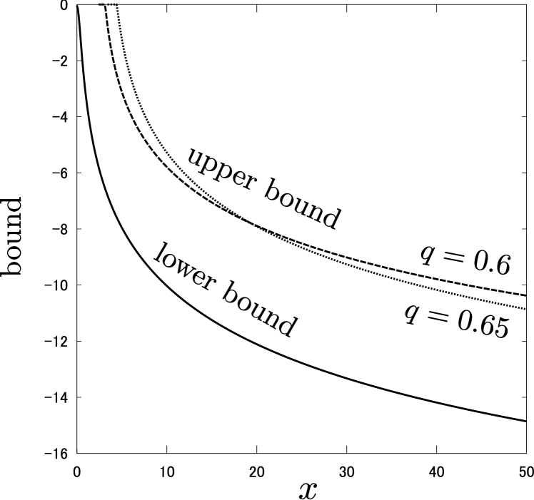
Figure 2: Lower bound (full line) and asymptotic upper bounds as a function of $x$ for the tail distribution of the sum of 5 i.i.d. variables distributed according to student t with $\nu=3$. The vertical axis shows the logarithm of the bounds. The parameters of the upper bounds are $q=0.6$ and $q=0.65$, respectively. In both cases is $a=5$.

7 Summary and Discussion

Our starting point is an application of the Markov inequality to variables of the form $\exp_{q}(aX)$, where $\exp_{q}$ is the $q$-deformed exponential function and $a>0$ is a free parameter. We use this to obtain an upper bound for sums of i.i.d. variables. In the case of a probability distribution with a compact support this leads to an elegant formalism which however is less powerful than the standard treatment. In the case of probability distributions with a fat tail we proceed by comparison with the $q^{*}$-deformed exponential distribution with $q^{*}=2-q$ and $0<q<1$. Large deviation estimates for the latter distribution are obtained from results found in the literature. Our main result is Theorem 6.5. It uses the analogy between the $q$-deformed and the standard exponential function to formulate a large deviation principle for distributions with a fat tail.

Is it worthwhile to introduce $q$-deformed exponential functions in the theory of large deviations? We know that there is no fundamental reason for their usage. The Lévy distributions are the appropriate tools for studying distributions with a fat tail. However, they are rather complicated. The main advantage of the $q^{*}$-deformed exponential distribution is therefore its simplicity. The possibility of proceeding by analogy with the conventional approach is a plus point. We interpret the standard theory of large deviations as a comparison of arbitrary distributions with the exponential distribution. Theorem 6.5 is based on a comparison of fat-tailed distributions with the $q^{*}$-deformed exponential distribution.

The present work is a first attempt to use $q$-deformed exponential functions in the context of large deviation theory. The main theorem is probably not optimal. The two examples serve as an illustration and fall short of showing the full potential of the present approach. Further work is therefore needed.

References

• [1] S.R.S. Varadhan, Asymptotic probabilities and differential equations, Commun. Pure Appl. Math. 19, 261–286 (1966).
• [2] R.S. Ellis, Entropy, Large Deviations, and Statistical Mechanics, (Springer, 1985)
• [3] J.-D. Deuschel, D.W. Stroock,Large Deviations (Academic Press, Duluth, 1989)
• [4] A. Dembo, O. Zeitouni, Large Deviations Techniques and Applications. 2nd Ed. (Springer, 1998)
• [5] F. den Hollander, Large Deviations. (Am. Math. Soc., Providence, 2000)
• [6] J. Feng and Th.G. Kurtz, Large Deviations for Stochastic Processes. Mathematical Surveys and Monographs, 131 (Am. Math. Soc., Providence, 2006)
• [7] H. Touchette, The large deviation approach to statistical mechanics, Phys. Rep. 478, 1 (2009).
• [8] C.C. Heyde, On large deviation probabilities for sums of random variables which are not attracted to the normal law, Ann. Math. Statist. 38, 1575 (1967).
• [9] C.C. Heyde, A contribution to the theory of large deviations for sums of independent random variables, Z. Wahrscheinlichkeitsth. 7 303 (1967).
• [10] A.V. Nagaev, Integral limit theorems for large deviations when Cramer’s condition is not fulfilled. I, II, Theory Prob. Appl. 14, 193–208 (1969).
• [11] A. V. Nagaev, Integral limit theorems taking into account large deviations when Cramer’s condition does not hold. I, II, Teor. Veroyatnost. i Primenen. 14, 51–63, 203–216 (1969).
• [12] S.V. Nagaev, Large deviations of sums of independent random variables, Ann. Prob. 7, 745 (1979).
• [13] L.V. Rozovski, Probabilities of large deviations on the whole axis, Theory Probab. Appl. 38, 53–79 (1993).
• [14] V. Vinogradov, Refined Large Deviation Limit Theorems, Pitman research notes in mathematics series 315 (Longman, Harlow, and John Wiley & Sons, Inc., New York, 1994)
• [15] C. KlΓΌppelberg , T. Mikosch, Large Deviations of Heavy-Tailed Random Sums With Applications in Insurance and Finance, (1997).
• [16] T. Mikosch, A.V. Nagaev, Large deviations of heavy-tailed sums with applications in insurance, Extremes 1, 81–110 (1998).
• [17] C. Su, Q. Tang, T. Jiang, A contribution to large deviations for heavy-tailed random sums, Science in China Series A: Mathematics, 44 438–444 (2001).
• [18] K.W. Ng, Q. Tang, J.A. Yan, H. Yang, Precise large deviations for sums of random variables with consistently varying tails, J. Appl. Prob. (2004).
• [19] Li Liu, Precise large deviations for dependent random variables with heavy tails, Stat. Prob. Lett. 79, 1290–1298 (2009).
• [20] C. Tsallis, What are the numbers that experiments provide? Quimica Nova 17, 468 (1994).
• [21] C. Tsallis, Possible Generalization of Boltzmann-Gibbs Statistics, J. Stat. Phys. 52, 479–487 (1988).
• [22] C. Tsallis, Introduction to nonextensive statistical mechanics (Springer Verlag, 2009).
• [23] J. Naudts, Generalised Thermostatistics (Springer Verlag, 2011).
• [24] G. Ruiz and C. Tsallis, Towards a large deviation theory for strongly correlated systems, Phys. Lett. A 376, 2451–2454 (2012).
• [25] H. Suyari, A.M. Scarfone, $\alpha$-divergence derived as the generalized rate function in a power-law system, http://arxiv.org/abs/1405.2562, Proc. ISITA2014, 130–134 (2014).
• [26] K. S. Lomax, Business Failures: Another Example of the Analysis of Failure Data, J. Am. Stat. Assoc. 49, 847–852 (1954).
• [27] J.L. Teugels, The class of subexponential distributions, Ann. Prob. 3, 1000–1011 (1975).