Approximation Schemes for Partitioning: Convex Decomposition and Surface Approximation

We revisit two NP-hard geometric partitioning problems – convex decomposition and surface approximation. Building on recent developments in geometric separators, we present quasi-polynomial time algorithms for these problems with improved approximation guarantees.

1 Introduction

The size and complexity of geometric objects are steadily growing due to the technological advancement of the tools that generate these. A simple strategy to deal with large, complex objects is to model them using pieces which are easy to handle. However, one must be careful while applying this kind of strategy as such decompositions are costly to construct and may generate a plethora of components. In this paper, we study two geometric optimization problems which deal with representations of complex models using simpler structures.

1.1 Polygon Decomposition Problem

The problem of decomposing a polygon into simpler pieces has a wide range of applications in VLSI, Robotics, Graphics, and Image Processing. Decomposition of complex polygons into convex pieces make them suitable for applications like skeleton extraction, mesh generation, and many others [5, 18, 31]. Considering the importance of this problem it has been studied for more than thirty years. Different versions of this problem have been considered based on the way of decomposition. The version we consider in this paper, which we refer to as the convex decomposition problem, is defined as follows.

Convex Decomposition Problem:

Let $P$ be a polygon possibly with polygonal holes. A diagonal in such a polygon is a line segment connecting two non-consecutive vertices that lies inside the polygon. The Convex Decomposition Problem is to add a set of non-crossing diagonals so that each subpolygon in the resulting decomposition of $P$ is convex, and the number of subpolygons is minimized.

For the polygons without holes, this problem can be solved in $O(r^{2}n\log n)$ time using a dynamic programming based approach, where $r$ is the number of reflex vertices [25]. Additionally, the running time could be improved to $O(n+r^{2}\min\{r^{2},n\})$ [26]. However, the problem is $\mathcal{NP}$-Hard if the polygon contains holes [32]. Hence Chazelle [9] gave a 4.333 factor approximation algorithm by applying a separator theorem recursively. Later, Hertel and Mehlhorn [23] improved the approximation factor to 4 by applying a simple strategy based on triangulation.

Many other versions of the polygon decomposition problem have also been studied. One of these versions allows the algorithm to add additional points inside the polygon. The endpoints of the line segments which decompose the polygon can be chosen from these additional points and the polygon vertices. Considering this version Chazelle and Dobkin [11] have designed an $O(n^{3})$ time optimal algorithm for the simple polygons without holes. Later, they improved the running time to $O(n+r^{3})$, where $r$ is the number of reflex angles [12, 10]. But, the problem is still $\mathcal{NP}$-Hard for polygons with holes [32]. In a different version the polygon is decomposed into approximately convex pieces where concavities are allowed within some specified tolerance [20, 28, 29, 30]. The idea is that these approximate convex pieces can be computed efficiently and can result in a smaller number of pieces. Another interesting variant is to consider an additional set of points inside the polygon and try to find the minimum number of convex pieces such that each piece contains at most $k$ such points, for a given $k$ [27].

1.2 Surface Approximation Problem

In many scientific disciplines including Computer Graphics, Image Processing, and Geographical Information System (GIS), surfaces are used for representation of geometric objects. Thus modeling of surfaces is a core problem in these areas, and polygonal descriptions are generally used for this purpose. However, considering the complexity of the input objects the goal is to use a minimal amount of polygonal description.

In many scientific computations 3D-object models are used. In that case the surface is approximated using piecewise linear patches (i.e, polygonal objects) whose vertices are allowed to lie within a close vicinity of the actual surface. To ensure that the local features of the original surface are retained, one may end up generating an unmanagable number of patches. But, this is not at all cost effective for real time applications. Thus one can clearly note the complexity-quality tradeoff in this context.

We consider the surface approximation problem for $xy$-monotone surfaces. The original surface is the graph of a continuous bivariate function $f(x,y)$ whose domain is $\mathbb{R}^{2}$. The goal is to compute a piecewise-linear function $g(x,y)$ which approximate the function $f(x,y)$. The domain of $g(\cdot,\cdot)$ is also $\mathbb{R}^{2}$, and we wish to minimize the number of its faces, which we require to be triangles. We formally define the problem as follows.

Surface Approximation Problem:

Let $f$ be a bivariate function and $\bar{S}$ be a set of $n$ points sampled from $f$. Given $\mu>0$ a piecewise linear function $g$ is called an $\mu$-approximation of $f$ if

$$|g(x_{i},y_{i})-z_{i}|\leq\mu$$

for every point $(x_{i},y_{i},z_{i})\in\bar{S}$. The surface approximation problem is to compute, given $f$ and $\mu$, such a $g$ with minimum complexity, where the complexity of a piecewise linear surface is defined to be the number of its faces.

Considering its importance there has been a lot of work on this problem in computer graphics and image processing [14, 16, 24, 36]. However, most of these approaches are based on heuristics and don’t give any guarantees on the solution. There are two basic techniques which are used by these algorithms: refinement and decimation. The former method starts with a triangle and further refine it locally until the solution becomes an $\mu$-approximation. The latter starts with a triangulation and coarsens it locally until one can’t remove a vertex [15, 19, 35].

The first provable guarantees for this problem were given by Agarwal and Suri. They gave an algorithm which computes an approximation of size $O(c\log c)$, and runs in $O(n^{8})$ time, where $c$ is the complexity of the optimal $\mu$-approximation [4]. They also proved that the decision version of this problem is $\mathcal{NP}$-complete. In a later work Agarwal and Desikan [3] presented a randomized algorithm which computes an approximation of size $O(c^{2}\log^{2}c)$ in $O(n^{2+\delta}+c^{3}\log^{2}c\log\frac{n}{c})$ expected time, where $c$ is the complexity of the optimal $\mu$-approximation and $\delta$ is any arbitrary small positive number.

A different version of the surface approximation problem has also considered by Mitchell and Suri [33]. Given a convex polytope $P$ with $n$ vertices and $\mu>0$ they designed an $O(n^{3})$ time algorithm which computes a $O(c\log n)$ size convex polytope $Q$ such that $(1-\mu)P\leq Q\leq(1+\mu)P$, where $c$ is the size of such an optimal polytope. Later, this bound was improved independently by Clarkson [13] and Bronniman and Goodrich [7]. The latter presented an $O(nc(c+\log n)\log\frac{n}{c})$ time algorithm which computes a polytope $Q$ of size $O(c)$. The hardness bound for this version is still an open problem.

1.3 Our Results

We obtain a quasi-polynomial time approximation scheme (QPTAS) for the convex decomposition problem using a separator based approach. We show the existence of a suitable set of diagonals (our separator), which partitions the optimal solution in a balanced manner, and intersects with a small fraction of optimal solution. Moreover, the set of diagonals can be guessed from a quasi-polynomial sized family. We then show the existence of a near-optimal solution that respects the set of diagonals. As we explain below, this proof of the existence of a suitable diagonal set, and a near-optimal solution that respects it, are our main technical contribution.

The approximation scheme is now a straightforward application: guess a separator, recurse on the subpolygons. The recursion bottoms out when we reach a subpolygon for which the optimal convex decomposition has a small size. This base case can be detected and solved in quasi-polynomial time by an exhaustive search.

Our result builds on the recent breakthrough due to Adamaszek and Wiese [1, 2]. They presented a QPTAS for independent set of weighted axis parallel rectangles [1], and subsequently extended their approach to polygons with polylogarithmic many vertices [2]. Har-peled [21] simplified and generalized their result to polygons of arbitrary complexity. Mustafa et al. [34] also describe a simplification, other generalizations, and an application to obtain a QPTAS for computing a minimum weight set cover using pseudo-disks.

For our problem, these results [2, 21, 34] imply a separator that intersects a small number of convex polygons in the optimal decomposition and partitions the remaining convex polygons evenly. However, such a separator may pass through the holes of polygon, and its intersection with the polygon may not be a set of diagonals. How do we convert the separator into a set of diagonals that still partitions nicely? And how do we convert the optimal decomposition into a near-optimal decomposition that respects this diagonal set? These are the key questions we address in our work.

For the surface approximation problem, we describe a quasi-polynomial time algorithm that computes a surface whose complexity is within a multiplicative constant factor of the optimal surface. The main contribution is a reduction from the surface approximation problem to a planar problem of computing a disjoint set cover using a certain family of triangles. We design a QPTAS for the disjoint set cover problem using the separator based approach. While similar reductions have been used in previous work on this problem, our reduction increases the size of the solution by at most a (multipilicative) constant factor. Our family of triangles has a useful closure property that facilitates the working of the QPTAS. In this way, we get a quasi-polynomial time $O(1)$-factor approximation algorithm for the surface approximation problem.

2 Convex Decomposition

Recall that we are given a polygon $P$ with zero or more polygonal holes. A diagonal in such a polygon is a line segment between two non-adjacent vertices that lies entirely within the polygon. The problem is to add a set of non-crossing diagonals so that each subpolygon in the resulting decomposition of $P$ is convex, and the number of convex polygons is the minimum possible.

2.1 A Separator

A set $D$ of diagonals of polygon $P$ is said to be conforming for $P$ if no two diagonals in $D$ cross. The diagonals in $D$ naturally partition $P$ into a set of polygons $\{P_{1},P_{2},\ldots,P_{t}\}$.

Let $K(P)$ denote the number of convex polygons in an optimal diagonal-based convex decomposition of $P$.

Lemma 1.

Let $P$ be a polygon (possibly with holes) that has $n$ vertices, let $K=K(P)$, and $0<\delta<1$ be a parameter. If $K\geq\frac{c\log(1/\delta)}{\delta^{3}}$, where $c$ is a sufficiently large constant, we can compute, in $n^{O(1/\delta^{2})}$ time, a family ${\cal D}=\{D_{1},D_{2},\ldots,D_{t}\}$ of conforming sets of diagonals of $P$ with the following property: there exists a $1\leq i\leq t$ such that the diagonals in $D_{i}$ partition $P$ into polygons $P_{1},P_{2},\ldots,P_{s}$, so that (a) $K(P_{j})\leq(2/3+\delta)K$, and (b) $\sum_{j=1}^{s}K(P_{j})\leq(1+\delta)K$.

The rest of the section is devoted to the proof of the lemma, which proceeds in three major steps. Fix an optimal diagonal-based convex decomposition of $P$, and let ${\cal C}=\{C_{1},\ldots,C_{K}\}$ be the set of resulting convex polygons. In the first step, we argue that there is a polygonal cycle $\Sigma$ such that (a) the number of polygons in ${\cal C}$ that are contained inside (resp. outside) $\Sigma$ is at most $2K/3$, and (b) the number of polygons in ${\cal C}$ whose interiors are intersected by $\Sigma$ is at most $\delta K/30$. This step is similar to the constructions in [2, 21, 34], but we need to review some particulars of these constructions to identify information that will be needed in subsequent steps. Notice that $\Sigma$ may actually intersect the holes of the polygon $P$.

In the second step, we show how to convert $\Sigma$ into a conforming set of diagonals $D$ such that as far as being a separator for ${\cal C}$ is concerned, $D$ behaves like a proxy for $\Sigma$. As a result of this process, the number of diagonals in $D$ may be significantly larger than the number of edges in $\Sigma$. Nevertheless, $D$ is an easily computed function of $\Sigma$.

In the third step, we exploit the separator properties of $D$ to compute, from ${\cal C}$, a suitable convex decomposition of $P$ that respects the diagonals in $D$. With this overview, we are ready to describe the three steps.

Step 1:

We have already fixed an optimal diagonal-based convex decomposition of $P$, with ${\cal C}=\{C_{1},\ldots,C_{K}\}$ being the set of resulting convex polygons. Without loss of generality, assume that no two vertices of $P$ lie on a vertical line. For each convex polygon $C_{i}$, let $s_{i}$ denote the line segment connecting the leftmost and rightmost points of $C_{i}$. We call $s_{i}$ the representative segment of $C_{i}$. Notice that $s_{i}$ is either an edge of $P$ or a diagonal of $P$. Let $S=\{s_{1},s_{2},\ldots,s_{K}\}$. See parts (a) and (b) of Figure 1.

(a) Polygon $P$ (with hole) along with its optimal convex decomposition $\mathcal{C}$, the latter denoted using dashed lines.

(b) The representative segment $s_{i}$ of each polygon $C_{i}\in\mathcal{C}$ is shown. Segments shown using solid lines are the ones chosen in the sample $R$.

(c) Trapezoidal decomposition, shown in dotted lines, of the segments in $R$. The separator $\Sigma$ is the dashed polygonal cycle $a$-$b$-$c$-$d$-$e$-$f$-$g$-$h$.

(d) The seperator $\Sigma$ and the polygon $P$.

Figure 1: Step 1 of the proof of Lemma 1

Let us fix an axes parallel box $B$ that contains $P$. Let us pick a random subset $R\subseteq S$ of size $\lceil r\log r\rceil\leq K$, where $r$ is a parameter that we fix below. We compute the trapezoidal decomposition, restricted to $B$, of the segments in $R$. (See Figure 1(c).) That is, from each endpoint $p$ of a segment in $R$, we shoot a vertical ray upwards (resp. downwards) till it hits either one of the other segments in $R$ or the boundary of $B$. We refer to the point that the ray hits as $u_{p}$ (resp. $d_{p}$). The vertical segments thus generated partition $B$ into faces, each of which is a trapezoid. The trapezoidal decomposition can be viewed as a planar graph whose faces correspond to the trapezoids. The vertices of this planar graph are the endpoints of segments in $R$, the vertices of $B$, and the points of the form $u_{p}$ or $d_{p}$. There are two types of edges – non-vertical and vertical. An edge that is contained within a segment $s\in R$ is a line segment connecting two consecutive vertices that lie in $s$. Similarly, there is an edge connecting every two consecutive vertices on the top (and bottom) edge of $B$. These edges constitute the non-vertical type. The vertical edges include ones of the form $\overline{pu_{p}}$ (resp. $\overline{pd_{p}}$), where $p$ is an endpoint of a segment in $S$. The left and right edges of $B$, which will also be edges of the planar graph, are included in the vertical category as well. The number of vertices, edges, and faces of the trapezoidal decomposition is $O(r\log r)$.

Notice that a nonvertical edge lying on the boundary of $B$ does not intersect any convex polygon in ${\cal C}$. Any other nonvertical edge intersects the interior of only the convex polygon whose representative segment it lies on. No nonvertical edge intersects the interior of any hole of $P$. A vertical edge, on the other hand, can intersect the interior of several convex polygons in ${\cal C}$ as well as the interiors of several holes. Note however, that a vertical edge intersects the interior of a convex polygon in ${\cal C}$ if and only if it intersects the relative interior of the corresponding representative segment. By standard sampling theory, there exists a choice of $R$, such that the number of convex polygons in ${\cal C}$ (representative segments in $S$) intersected by any vertical edge in the trapezoidal decomposition of $R$ is at most $c_{1}K/r$, for some constant $c_{1}>0$. We will assume henceforth that $R$ satisfies this property.

Let $n(e)$ denote the number of convex polygons whose interiors are intersected by edge $e$ of the trapezoidal decomposition.

Recall that the trapezoidal decomposition of $R$ is a planar graph with $O(r\log r)$ vertices, edges, and faces. The articles [2, 21, 34] study separators which are simple polygonal cycles whose edges are the edges of the planar graph. In particular, the arguments of [2, 21, 34] imply that there is a simple polygonal cycle $\Sigma$ in the plane, constituted of $O(\sqrt{r\log r})$ edges of the trapezoidal decomposition, such that (a) the number of representative segments (convex polygons) in the interior of $\Sigma$ is at most $2K/3$, and (b) the number of representative segments (convex polygons) in the exterior of $\Sigma$ is at most $2K/3$. See Figure 1(d). Let ${\cal C}^{\text{int}}$ (resp. ${\cal C}^{\text{ext}}$) denote the subset consisting of those polygons of ${\cal C}$ in the interior (resp. exterior) of $\Sigma$. Abusing notation, we say $e\in\Sigma$ to mean that $e$ is an edge of the trapezoidal decomposition that is contained in $\Sigma$. We have that $\sum_{e\in\Sigma}n(e)\leq O(\sqrt{r\log r})\frac{c_{1}K}{r}$. We will choose $r$ large enough so that

$$30\sum_{e\in\Sigma}n(e)\leq\delta K.$$ (1)

This can be ensured by, say, setting $r=c/\delta^{3}$ for sufficiently large constant $c$. Then $\Sigma$ would be constituted of $O(1/\delta^{2})$ edges of the trapezoidal decomposition. Each vertex of such an edge is specified by a tuple consisting of $O(1)$ features of the input polygon – note that a vertex of the form of $u_{p}$ or $d_{p}$ is specified by $p$ and a representative segment, which is a diagonal or edge of the input polygon. Thus $\Sigma$ can be specified by $O(1/\delta^{2})$ such tuples. This implies that there is an algorithm, that, given $P$, computes in $n^{O(1/\delta^{2})}$ time a family of $n^{O(1/\delta^{2})}$ cycles that contains a $\Sigma$ satisfying (1).

Step 2:

We delete from $\Sigma$ the portions that lie in the interiors of the holes (this includes the unbounded hole outside $P$ as well). That is, we consider $\Sigma\cap P$. We further partition each connected component of $\Sigma\cap P$ using the vertices of $P$ that lie in the relative interior of the component. See Figure 2. This partitions $\Sigma\cap P$ into fragments, which are polygonal chains. An endpoint of such a chain is either a vertex of $P$ or a point $q$ that lies in the interior of an edge $f$ of the polygon. Let $\Sigma^{\prime}$ denote the resulting collection of fragments. Each fragment $\sigma$ contains at most two vertical edges (which would be portions of vertical edges in $\Sigma$) and at most one nonvertical edge (which would be part of some representative segment, and made up of one or more edges of the trapezoidal decomposition that are contiguous on that segment). For a convex polygon $C\in{\cal C}$, let $n(\sigma,C)$ denote the number of connected components of $\sigma\cap(\text{interior}\ C)$. The quantity $n(\sigma,C)$ is either $0$, $1$, or $2$ – we can get two components if $\sigma$ actually has two vertical edges that both intersect $C$. Let $n(\sigma)=\sum_{C\in{\cal C}}n(\sigma,C)$.

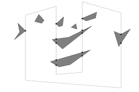
Figure 2: (a) The separator $\Sigma$ which may pass through polygon holes, which are shaded. (b) The fragments in $\Sigma\cap P$.

We slightly modify fragment $\sigma$ so that both its endpoints are vertices of $P$: if an endpoint of $\sigma$ is a point $p$ on the interior of edge $f$ of the polygon $P$, we extend $\sigma$ by adding the segment from $p$ to the left endpoint of $f$. See Figure 3. Note that $n(\sigma,C)$ remains unchanged as a consequence of this. The set $\Sigma^{\prime}$ of fragments now satisfies the following properties:

1. $\sum_{\sigma\in\Sigma^{\prime}}n(\sigma)\leq\sum_{e\in\Sigma}n(e)\leq\delta K/30$.

2. Each fragment $\sigma\in\Sigma^{\prime}$ begins and ends at a vertex of $P$ and contains no vertex of $P$ in its relative interior.

3. No fragment in $\Sigma^{\prime}$ intersects the interior of any convex polygon in ${\cal C}^{\text{int}}\cup{\cal C}^{\text{ext}}$.

4. The fragments in $\Sigma^{\prime}$ partition $P$ into connected components with the property that no component contains a polygon from ${\cal C}^{\text{int}}$ as well as a polygon from ${\cal C}^{\text{ext}}$. (That is, a component may contain polygons from ${\cal C}^{\text{int}}$, or polygons from ${\cal C}^{\text{ext}}$, but not polygons from both ${\cal C}^{\text{int}}$ and ${\cal C}^{\text{ext}}$.)

5. Each fragment $\sigma\in\Sigma^{\prime}$ is not self-intersecting. However, the two endpoints of a fragment may be the same point.

6. No two fragments in $\Sigma^{\prime}$ cross.

Figure 3: (a) Modifying each fragment so that endpoints are polygon vertices. (b) The diagonals resulting from replacing each fragment by a shortest homotopic path.

For each $\sigma\in\Sigma^{\prime}$, we compute the shortest path $\overline{\sigma}$ in $P$ between the endpoints of $\sigma$ that is homotopic to $\sigma$. This can be done efficiently [22, 17, 8, 6]. Let us denote by $n(\overline{\sigma},C)$ the number of connected components of $\overline{\sigma}\cap(\text{interior }\ C)$, for any $C\in{\cal C}$. Then we have $n(\overline{\sigma},C)\leq n(\sigma,C)$ for any polygon $C\in{\cal C}$. In particular, if the interior of $C$ is not intersected by $\sigma$ then it is not intersected by $\overline{\sigma}$ as well. Let $n(\overline{\sigma})=\sum_{C\in{\cal C}}n(\overline{\sigma},C)$.

Let $\overline{\Sigma}=\{\overline{\sigma}\ |\ \sigma\in\Sigma^{\prime}$}. The fragments in $\overline{\Sigma}$ satisfy the following properties:

1. $\sum_{\overline{\sigma}\in\overline{\Sigma}}n(\overline{\sigma})\leq\sum_{e\in\Sigma}n(e)\leq\delta K/30$.

2. Each fragment $\overline{\sigma}\in\overline{\Sigma}$ begins and ends at a vertex of $P$ and contains no vertex of $P$ in its relative interior.

3. No fragment in $\overline{\Sigma}$ intersects the interior of any convex polygon in ${\cal C}^{\text{int}}\cup{\cal C}^{\text{ext}}$.

4. The removal of the points corresponding to the fragments in $\overline{\Sigma}$ partitions $P$ into connected components with the property that no component contains a polygon from ${\cal C}^{\text{int}}$ as well as a polygon from ${\cal C}^{\text{ext}}$.

5. Each fragment $\overline{\sigma}\in\overline{\Sigma}$ is not self-intersecting. However, the two endpoints of a fragment may be the same point.

6. No two fragments in $\overline{\Sigma}$ cross.

Note that each fragment $\overline{\sigma}$, being a shortest homotopic path, is constituted of a sequence of diagonals and edges from $P$. So we define $D(\Sigma)$ as the set of diagonals corresponding to the fragments in $\overline{\Sigma}$. (A diagonal in $D(\Sigma)$ can be present in more than one fragment of $\overline{\Sigma}$.) See Figure 3.

The last two fragment properties of $\overline{\Sigma}$ imply that $D(\Sigma)$ is a conforming set of diagonals. Notice that the number of diagonals in $D(\Sigma)$ can be much greater than the number of edges in $\Sigma$. However, $D(\Sigma)$ is uniquely and efficiently computed given $\Sigma$. Since $\Sigma$ comes from a family of $n^{O(1/\delta^{2})}$ cycles that can be computed in $n^{O(1/\delta^{2})}$ time given $P$, $D(\Sigma)$ comes from a family of $n^{O(1/\delta^{2})}$ diagonal subsets that can be computed in $n^{O(1/\delta^{2})}$ time given $P$.

Step 3:

For a diagonal $d\in D(\Sigma)$, let $n(d,C)=1$ if $d$ intersects the interior of $C\in{\cal C}$, and $0$ otherwise. Let $n(d)=\sum_{C\in{\cal C}}n(d,C)$. The first property of $\overline{\Sigma}$ can be restated as saying that $\sum_{d\in D(\Sigma)}n(d)\leq\delta K/30$.

The diagonals in $D(\Sigma)$ partition $P$ into a set of smaller polygons $\{P_{1},P_{2},\ldots,P_{s}\}$. We now show how to obtain, from ${\cal C}$, convex decompositions of these smaller polygons that obey the size bounds claimed in the lemma. We will think of these new convex decompositions as a new convex decomposition of $P$ that respects the set $D(\Sigma)$ of diagonals. The new convex decomposition will have the convex polygons in ${\cal C}^{\text{int}}$ and ${\cal C}^{\text{ext}}$ – the interiors of these polygons do not intersect the diagonals in $D(\Sigma)$. Let ${\cal C}^{\text{bad}}={\cal C}\setminus\{{\cal C}^{\text{int}}\cup{\cal C}^{\text{ext}}\}$. From the properties of $\Sigma$, it follows that $|{\cal C}^{\text{bad}}|\leq\delta K/30$. We show below that we can obtain a convex decomposition of size at most $\delta K$ for the portion of $P$ that is covered by the polygons in ${\cal C}^{\text{bad}}$. This convex decomposition will respect the set $D(\Sigma)$. Since smaller polygon $P_{j}$ does not have a polygon from both ${\cal C}^{\text{int}}$ and ${\cal C}^{\text{ext}}$, it follows that

$$K(P_{j})\leq\max\{|{\cal C}^{\text{int}}|,|{\cal C}^{\text{ext}}|\}+\delta K\leq(2/3+\delta)K.$$

It also follows that

$$\sum_{j}K(P_{j})\leq|{\cal C}^{\text{int}}|+|{\cal C}^{\text{ext}}|+\delta K\leq(1+\delta)K.$$

We describe the construction of ${\cal C}^{\text{new}}$, the new convex decomposition of the portion of $P$ that is covered by the polygons in ${\cal C}^{\text{bad}}$. This ${\cal C}^{\text{new}}$ respects the diagonals in $D(\Sigma)$, that is, the interior of no convex polygon in ${\cal C}^{\text{new}}$ is intersected by a diagonal in $D(\Sigma)$. For each convex polygon $C\in{\cal C}^{\text{bad}}$, consider the subset $D(C)\subseteq D(\Sigma)$ of diagonals that intersect the interior of $C$. Let $V(C)$ denote those vertices of $C$ that do not lie on any diagonal in $D(\Sigma)$. Define the following relation on $V(C)$: $u$ and $v$ are related if the line segment joining them does not intersect any diagonal in $D(C)$. It is easy to see that this is an equivalence relation. Let $V_{1},V_{2},\ldots,V_{m}$ be the equivalence classes. It is easy to see that $m\leq D(C)+1$. We add $\text{Conv}(V_{i})$ to ${\cal C}^{\text{new}}$ if $\text{Conv}(V_{i})$ is a 2-dimensional object, that is, not a line segment or a point. See Figure  4. The number of convex polygons contributed by $C$ to ${\cal C}^{\text{new}}$ is at most $1+D(C)$, so the number of convex polygons in ${\cal C}^{\text{new}}$ overall is at most

$$\sum_{C\in{\cal C}^{\text{bad}}}(1+D(C))\leq|{\cal C}^{\text{bad}}|+\sum_{d\in D(\Sigma)}n(d)\leq\delta K/15.$$

Figure 4: (a) A convex polygon $C\in{\cal C}^{\text{bad}}$, and the diagonals in $D(\Sigma)$ that intersect it. (b) The convex polygons added to ${\cal C}^{\text{new}}$ from $C$.

For each polygon $P_{j}$ in the partition of $P$ induced by $D(\Sigma)$, consider the portion that is outside the polygons of ${\cal C}^{\text{int}}$, ${\cal C}^{\text{ext}}$, and ${\cal C}^{\text{new}}$. This portion is a set of polygons. We triangulate each such polygon, and add the resulting triangles to ${\cal C}^{\text{new}}$. See Figure 5. Note that triangulating a polygon with $m$ vertices results in at most $3m$ triangles, even if the polygon has holes. This completes the construction of ${\cal C}^{\text{new}}$.

We need to bound the number of triangles added in this step, summed over all $P_{j}$. To this end, let $\lambda$ denote the sum of the number of vertices of all the polygons we triangulate. To bound $\lambda$, we observe that each $C\in{\cal C}^{\text{bad}}$ “contributes” at most $8D(C)$ vertex-polygon features to $\lambda$. Thus, $\lambda\leq 8\sum_{C\in{\cal C}^{\text{bad}}}D(C)\leq 8\delta K/30$. So the number of triangles we add to ${\cal C}^{\text{new}}$ is at most $3\lambda\leq 24\delta K/30$.

Thus, $|{\cal C}^{\text{new}}|\leq\frac{24\delta K}{30}+\frac{\delta K}{15}\leq\delta K$. We now have the desired convex decomposition of $P$ that respects $D(\Sigma)$: ${\cal C}^{\text{int}}\cup{\cal C}^{\text{ext}}\cup{\cal C}^{\text{new}}$. This completes the proof of the lemma.

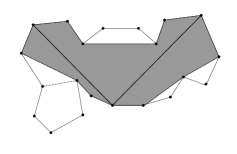
Figure 5: (a) An illustration of a polygon $P$, an optimal decomposition ${\cal C}$ using (dashed) diagonals, and the two diagonals in $D(\Sigma)$ (bold). (b) The three polygons in ${\cal C}^{\text{bad}}$ contribute a total of four convex polygons to ${\cal C}^{\text{new}}$; in addition, we triangulate the shaded polygons and add the triangles to ${\cal C}^{\text{new}}$.

2.2 Algorithmic Aspects

We now use the Lemma 1 to develop a QPTAS for the convex decomposition problem. For this purpose, we need a good exact algorithm to serve as the base case for our recursive algorithm. Suppose $P^{\prime}$ is an $n$-vertex polygon, and the optimal decomposition for it has $K=K(P^{\prime})$ convex polygons $P^{\prime}_{1},\ldots,P^{\prime}_{k}$. We argue that the number of diagonals added is at most $3K-6$. To see this, construct a graph where there is a vertex for each $P^{\prime}_{i}$, and an edge for each diagonal between the (vertices corresponding to the ) two convex polygons it is incident to. This graph is clearly planar. Furthermore, since the $P^{\prime}_{i}$ are convex, the graph has no parallel edges. As such, the number of edges, and hence diagonals, is at most $3K-6$.

Thus, given an $n$-vertex polygon $P^{\prime}$ and a $k\geq 0$, we can check if $P^{\prime}$ admits a convex decomposition of size at most $k$ in $n^{O(k)}$ time. We only need to try all conforming subsets of at most $3k-6$ diagonals. In the same time bound, we can find an optimal convex decomposition, assuming it has size at most $k$.

We now describe our QPTAS. It will be convenient to describe a non-deterministic algorithm first. Assuming it makes the right separator choices, we can analyze the approximation guarantee. Subsequently, we make the algorithm deterministic and bound its running time.

Nondeterministic Algorithm.

Our algorithm $\text{decompose}(P^{\prime})$ takes as input a polygon $P^{\prime}$ and returns a decomposition of $P^{\prime}$. It uses a parameter $0<\delta<\frac{3}{4}-\frac{2}{3}$ that we specify later. Let $\lambda=\frac{c\log(1/\delta)}{\delta^{3}}$, the threshold in Lemma 1. Since $P^{\prime}$ will be a subpolygon of $P$, the number of its vertices is at most $n$. Our overall algorithm simply invokes $\text{decompose}(P)$.

1. We check if $P^{\prime}$ has a decomposition with at most $\lambda$ convex polygons. If so, we return the optimal decomposition. This is the base case of our algorithm. This computation can be done as described above in $n^{O(\lambda)}$ time. Henceforth, we assume that $K(P^{\prime})>\lambda$.

2. Compute the family ${\cal D}=\{D_{1},D_{2},\ldots,D_{t}\}$ of sets of diagonals, as stated in Lemma 1, for $P^{\prime}$.

3. Choose a $D_{i}\in{\cal D}$.

4. Suppose $D_{i}$ partitions $P^{\prime}$ into subpolygons $P^{\prime}_{1},P^{\prime}_{2},\ldots,P^{\prime}_{s}$. Return

   $$\bigcup_{j=1}^{s}\text{decompose}(P^{\prime}_{j}).$$

Approximation Ratio.

We define the level of a polygon $P^{\prime}$ to be the integer $i>0$ such that $\lambda(4/3)^{i-1}<K(P^{\prime})\leq\lambda(4/3)^{i}$. If $K(P^{\prime})\leq\lambda$, we define its level to be $0$. Thus if $\text{decompose}(P^{\prime})$ is solved via the base case, then the level of $P^{\prime}$ is $0$. The following lemma bounds the quality of approximation of our non-deterministic algorithm.

Lemma 2.

Assume that $\delta<\frac{3}{4}-\frac{2}{3}$. There is an instantiation of the non-deterministic choices for which $\text{decompose}(P^{\prime})$ returns a convex decomposition with at most $(1+\delta)^{\ell}K(P^{\prime})$ polygons, where $\ell$ is the level of $P^{\prime}$.

Proof.

The proof is by induction on $\ell$. The base case is when $\ell=0$, and here the statement follows from the base case of the algorithm. So assume that $\ell>1$, and that the statement holds for instances with level at most $\ell-1$.

Suppose that the algorithm non-deterministcally picks the $D_{i}\in{\cal D}$ that satisfies the guarantees of Lemma 1 for $P^{\prime}$. Let $P^{\prime}_{1},P^{\prime}_{2},\ldots,P^{\prime}_{s}$ be the subpolygons that result from partitioning $P^{\prime}$ with $D_{i}$.

Since $K(P^{\prime}_{j})\leq(2/3+\delta)K(P^{\prime})\leq(3/4)K(P^{\prime})$, it follows that the level of each $P^{\prime}_{j}$ is at most $\ell-1$. Thus, for each $j$, there are nondeterministic choices for which $\text{decompose}(P^{\prime}_{j})$ returns a decomposition of $P^{\prime}_{j}$ with at most $(1+\delta)^{\ell-1}K(P^{\prime}_{j})$ polygons. Thus, the size of the decomposition of $P^{\prime}$ returned by $\text{decompose}(P^{\prime})$ is at most

$$(1+\delta)^{\ell-1}\sum_{j}K(P^{\prime}_{j})\leq(1+\delta)^{\ell}K(P^{\prime}).$$

∎

Deterministic Algorithm.

Since a triangulation of $P$, the original input polygon, uses at most $3n-6$ triangles, the level of $P$ is at most $\alpha=\log_{4/3}(3n-6)$. It follows that with $\text{decompose}(P)$, for suitable non-deterministic separator choices, returns a decomposition with at most $(1+\delta)^{\alpha}$ times the size of the optimal disjoint cover. Furthermore, the depth of the recursion with such seperator choices is at most $\alpha$.

To get a deterministic algorithm, we make the following natural changes to $\text{decompose}(P^{\prime})$. If a call to $\text{decompose}(P^{\prime})$ is at recursion depth that is greater than $\alpha$ (with respect to the root corresponding to $\text{decompose}(P)$), we return a special symbol $I$. In the $\text{decompose}(P^{\prime})$ routine, when we are not in the base case, we try all possible separators $D_{i}\in{\cal D}$ instead of nondeterministically guessing one – we return the smallest sized set $\bigcup_{j=1}^{s}\text{decompose}(P^{\prime}_{j})$, over all $i$ for which none of the recursive calls $\text{decompose}(P^{\prime}_{j})$ returns $I$. If no such $i$ exists, $\text{decompose}(P^{\prime})$ returns $I$.

With these changes, $\text{decompose}(P)$ is now a deterministic algorithm that returns a decomposition of size at most $(1+\delta)^{\alpha}K(P)$. Its running time is

$$\left(n^{O(1/\delta^{2})}\right)^{\alpha}\cdot n^{O(\lambda)}=n^{O\left((\log n+\log 1/\delta)/\delta^{3}\right)}.$$

Plugging $\delta=\varepsilon/2\alpha$, the approximation guarantee is $(1+\varepsilon)$ and the running time is $n^{O((\log n/\varepsilon)^{4})}$. We can thus conclude with our main result for convex decomposition:

Theorem 1.

There is an algorithm that, given a polygon $P$ and an $\varepsilon>0$, runs in time $n^{O((\log n/\varepsilon)^{4})}$ and returns a diagonal-based convex decomposition of $P$ with at most $(1+\varepsilon)K(P)$ polygons, where $K(P)$ is the number of polygons in an optimal diagonal-based convex decomposition of $P$. Here $n$ stands for the number of vertices in $P$.

3 Surface Approximation

We now describe our algorithm for the surface approximation problem. Recall that we are given a set $\bar{S}$ of $n$ points in $\mathbb{R}^{3}$ sampled from a bi-variate function $f(x,y)$, and another parameter $\mu>0$. A piece-wise linear function $g(x,y)$ is an approximation of $f(x,y)$ if $\forall\bar{p}=(x,y,z)\in\bar{S},|g(x,y)-z|\leq\mu$. The bi-variate function $f(x,y)$ represents the surface from which the points are sampled, and we want to compute an approximate polyhedral surface $g(x,y)$ with minimal complexity. The complexity of a piecewise linear surface is defined to be the number of its faces, which are required to be triangles.

For any point $\bar{p}\in\bar{S}$ which is in $\mathbb{R}^{3}$, we define $p$ to be the projection of $\bar{p}$ on to the $xy$-plane. Let $S=\{p\ |\ \bar{p}\in\bar{S}\}$. A triangle $\triangle$ in the $xy$-plane is a valid triangle if it is the projection of a triangle $\overline{\triangle}$ in $\mathbb{R}^{3}$, such that $\forall p\in S\cap\triangle$ the vertical distance between $\overline{\triangle}$ and $\bar{p}$ is at most $\mu$. Agarwal and Suri [4] have shown that the surface approximation problem is equivalent, up to multiplicative constant factors, to computing a minimum-cardinality cover for $S$ using a set of valid triangles with pairwise-disjoint interiors. Notice that the set of valid triangles can be infinite. We describe a method for computing a polynomial-sized set $\mathcal{B}$ of valid triangles, termed the basis, such that the surface approximation problem is equivalent, up to multiplicative constant factors, to computing a minimum-cardinality cover for $S$ using a subset of basis triangles with pairwise-disjoint interiors. As we then show, the basis triangles have a certain closure property that enables us to obtain an approximation scheme for the above covering problem using the seperator approach.

3.1 Construction of the basis

Let $\mathcal{T}$ be the set of all valid triangles in the plane, which can be infinite. Let ${\cal F}=\{S\cap\triangle\ |\ \triangle\mbox{ is a triangle}\}$. It is easy to see that set ${\cal F}$ has size $O(n^{6})$, and can be computed in, say, $O(n^{7})$ time.

Figure 6: (a) An arbitrary triangle $\triangle$ and the set $R=\triangle\cap S\in\mathcal{F}$. The dashed polygon is $\text{Conv}(R)$. (b) Three points $p,q,r$ on $\text{Conv}(R)$ and the corresponding hexagon $H_{pqr}$ formed by the edges of $\text{Conv}(R)$ incident on $p,q,r$. (c) Triangulation of $H_{pqr}$ results in the addition of at most 4 triangles to $\mathcal{B}$, which cover the points in $R$.

For each $R\in{\cal F}$, we compute the convex hull $\text{Conv}(R)$ of the points in $R$. If $\text{Conv}(R)$ consists of a point, or a single edge, we add the degenerate triangle $\text{Conv}(R)$ to the basis $\mathcal{B}$. Otherwise, $\text{Conv}(R)$ is 2-dimensional and has at least three vertices. For each triple $\{p,q,r\}$ of vertices in $\text{Conv}(R)$, we contruct the hexagon $H_{pqr}$ formed by the edges of $\text{Conv}(R)$ incident on $p$, $q$, and $r$. $H_{pqr}$ may be degenerate i.e. it may not be a hexagon, or it may be unbounded. In case $H_{pqr}$ is bounded, we triangulate the hexagon by using diagonals from the bottom vertex, and add the resulting set of at most $4$ triangles to $\mathcal{B}$. See Figure 6

Since we generate at most $O(n^{3})$ hexagons from $\text{Conv}(R)$, and from each such hexagon we generate at most $4$ triangles, the basis $\mathcal{B}$ would now consist of at most $O(n^{9})$ triangles.

Filtering the basis:

We remove any triangle ${\triangle}\in\mathcal{B}$ that is not a valid triangle. This can be done by solving a simple $3$-dimensional linear program for each triangle in $\mathcal{B}$, as shown by Agarwal and Desikan [3]. Let $S_{\triangle}=S\cap{\triangle}$ be the set of points contained inside ${\triangle}\in\mathcal{B}$. Since ${\triangle}$ is a valid triangle, then there would exist a triangle $\overline{\triangle}$ in $\mathbb{R}^{3}$ such that ${\triangle}$ is the projection of $\overline{\triangle}$ on the $xy$-plane, and the vertical distance between $\overline{\triangle}$ and any point in $\{\bar{p}\ |\ p\in S_{\triangle}\}$ is at most $\mu$. This completes the description of the basis computation.

A useful property of the basis is summarized below.

Lemma 3.

Let $\triangle$ be any valid triangle. There exist a set $\mathcal{B}(\triangle)\subseteq\mathcal{B}$ of at most four triangles, such that (a) the triangles in $\mathcal{B}(\triangle)$ have pair-wise disjoint interiors; (b) each of the triangles in $\mathcal{B}(\triangle)$ is contained in $\triangle$; and (c) $\mathcal{B}(\triangle)$ covers $S\cap\triangle$.

Proof.

Let $R=S\cap{\triangle}$. If $\text{Conv}(R)$ is $0$- or $1$-dimensional, we have added the degenerate triangle $\text{Conv}(R)$ itself to $\mathcal{B}$, and the lemma holds with $\mathcal{B}(\triangle)=\{\text{Conv}(R)\}$ . Assume henceforth that $\text{Conv}(R)$ is $2$-dimensional.

Let $h_{1},h_{2},h_{3}$ be the half-planes defined by the 3 edges of ${\triangle}$, such that $h_{1}\cap h_{2}\cap h_{3}={\triangle}$. Let $p_{i}$ be the point in $R$ that is closest to the line bounding $h_{i}$ – if there is a tie, we break it arbitrarily. Consider the hexagon $H_{p_{1}p_{2}p_{3}}$ formed by extending the edges of $\text{Conv}(R)$ incident to the $p_{i}$. Our procedure for generating the basis would have generated the hexagon $H_{p_{1}p_{2}p_{3}}$ while considering $R$. It is not hard to see, as we explain below, that $H_{p_{1}p_{2}p_{3}}\subseteq\triangle$. The set of at most $4$ triangles that we obtain by triangulating $H_{p_{1}p_{2}p_{3}}$ are added to $\mathcal{B}$. This set $\mathcal{B}(\triangle)$ of triangles has the properties claimed.

We now show that $H_{p_{1}p_{2}p_{3}}\subseteq\triangle$. Let $W_{i}$ be the wedge whose apex is at $p_{i}$ and whose bounding rays are the ones containing the two edges of $\text{Conv}(R)$ incident at $p_{i}$. Since $p_{i}$ is the point in $\text{Conv}(R)$ that is closest to the line bounding $h_{i}$, it follows that the two rays bounding the edge $W_{i}$ do not contain any point outside $h_{i}$. That is, $W_{i}\subseteq h_{i}$. This implies that

$$H_{p_{1}p_{2}p_{3}}=W_{1}\cap W_{2}\cap W_{3}\subseteq h_{1}\cap h_{2}\cap h_{3}=\triangle.$$

∎

The next two observations relate the surface approximation problem to that of computing a minimal cover of $S$ using a set of pairwise-disjoint triangles from the basis $\mathcal{B}$. A consequence of our basis if the following.

Lemma 4.

There is a set of at most $4OPT$ triangles from $\mathcal{B}$, with pairwise-disjoint interiors, that covers $S$, where $OPT$ is the complexity of an optimal solution to our surface approximation instance.

Proof.

Consider the set $\mathcal{T}^{\prime}\subseteq\mathcal{T}$ of triangles that are formed by projecting the triangular faces in the optimal solution. The set $\bigcup_{\triangle\in\mathcal{T}^{\prime}}\mathcal{B}(\triangle)$ has the properties claimed. ∎

The next observation is due to Agarwal and Suri [4].

Lemma 5.

If we have a cover of $S$ using $m$ pairwise-disjoint triangles from $\mathcal{T}$, then we can efficiently compute a solution to the surface approximation problem with complexity $O(m)$.

The above two lemmas imply that if we have an $O(1)$-approximation to the problem of computing a minimal cover of $S$ using a set of pairwise-disjoint triangles from the basis $\mathcal{B}$, then we have an $O(1)$-approximation for the original surface approximation problem.

3.2 A Disjoint Cover Using Basis Triangles

We now describe a QPTAS for the problem of computing the smallest pair-wise disjoint subset of ${\cal B}$ that covers $S$.

The Separator.

We need the following separator computation, which is very similar to the constructions in [2, 21, 34] and Step 1 of the separator theorem for convex decomposition. Our separators will be closed, simple, polygonal curves. For an edge $e$ on such a curve $C$, and for a pairwise-disjoint subset ${\cal D}\subseteq{\cal B}$, let $n(e,{\cal D})$ denote the number of triangles in ${\cal D}$ whose relative interior is intersected by $e$, and let $n(C,{\cal D})$ denote $\sum_{e}n(e,{\cal D})$, where the summation is over all edges $e$ of $C$.

Lemma 6.

Given ${\cal B}$, and $0<\delta<1$, we can compute in time $n^{O(1/\delta^{2})}$ a family ${\cal C}=\{C_{1},C_{2},\ldots,C_{t}\}$ of closed, simple, polygonal curves, each with $O(1/\delta^{2})$ vertices, with the following property: for any subset ${\cal D}\subseteq{\cal B}$ with pairwise-disjoint triangles such that $K:=|{\cal D}|\geq\lambda:=\frac{c\log 1/\delta}{\delta^{3}}$, there is a $C_{j}\in{\cal C}$ such that (a) $n(C_{j},{\cal D})\leq\delta K/10$; (b) the number of triangles of ${\cal D}$ inside $C_{j}$ is at most $\frac{2K}{3}$; and (c) the number of triangles of ${\cal D}$ outside $C_{j}$ is at most $\frac{2K}{3}$.

The Algorithm.

We describe a recursive procedure $\text{compcover}(S^{\prime},{\cal B}^{\prime})$ that given as input subsets $S^{\prime}\subseteq S$ and ${\cal B}^{\prime}\subseteq{\cal B}$, returns a cover of $S^{\prime}$ with a set of pairwise disjoint triangles from ${\cal B}^{\prime}$. We assume that ${\cal B}^{\prime}$ has the following closure property: if $\triangle\in{\cal B}^{\prime}$, and $\triangle_{1}\in{\cal B}$ is contained in $\triangle$, then $\triangle_{1}\in{\cal B}^{\prime}$ as well. Our final algorithm simply invokes $\text{compcover}(S,{\cal B})$. Our algorithm $\text{compcover}(S^{\prime},{\cal B}^{\prime})$ is non-deterministic in the step in which it makes a choice of separator. After analyzing the quality of the solution produced by this non-deterministic algorithm, for suitable separator choices, we discuss how it can be made deterministic.

1. By exhaustive search, we check if there is a subset of ${\cal B}^{\prime}$ with at most $\lambda=c\frac{\log 1/\delta}{\delta^{3}}$ pairwise disjoint triangles that covers $S^{\prime}$. If so, we return such a subset with minimum cardinality. This is the base case of our algorithm. Henceforth, we assume that a minimal pairwise-disjoint cover needs at least $\lambda=\frac{c\log 1/\delta}{\delta^{3}}$ triangles.

2. Choose a separator $C_{j}\in{\cal C}$.

3. Let $S^{\prime}_{j1}$ be the set of points in $S^{\prime}$ that are inside $C_{j}$, and let $S^{\prime}_{j2}$ be the remaining points in $S^{\prime}$. Let ${\cal B}^{\prime}_{j1}$ denote those triangles of ${\cal B}^{\prime}$ that are inside $C_{j}$, and ${\cal B}^{\prime}_{j2}$ denote those triangles of ${\cal B}^{\prime}$ that are outside $C_{j}$.

4. Return $\text{compcover}(S^{\prime}_{j1},{\cal B}^{\prime}_{j1})\cup\text{compcover}(S^{\prime}_{j2},{\cal B}^{\prime}_{j2})$.

We note that ${\cal B}^{\prime}_{j1}$ and ${\cal B}^{\prime}_{j2}$ satisfy the closure property that ${\cal B}^{\prime}$ has.

Approximation Ratio.

Consider an input $(S^{\prime},{\cal B}^{\prime})$ to our algorithm, and suppose ${\cal D}^{\prime}\subseteq{\cal B}^{\prime}$ is a smallest pairwise-disjoint subset of ${\cal B}^{\prime}$ that covers $S^{\prime}$. We define the level of the instance $(S^{\prime},{\cal B}^{\prime})$ to be the integer $i>0$ such that $\lambda(4/3)^{i-1}<|{\cal D}^{\prime}|\leq\lambda(4/3)^{i}$. If $|{\cal D}^{\prime}|<\lambda$, we define its level to be $0$ – thus a base case input $(S^{\prime},{\cal B}^{\prime})$ has level $0$. The following lemma bounds the quality of approximation of our non-deterministic algorithm.

Lemma 7.

Assume that $\delta<3/4-2/3$. There is an instantiation of the non-deterministic separator choices for which $\text{compcover}(S^{\prime},{\cal B}^{\prime})$ computes a disjoint cover of size at most $(1+\delta)^{i}|{\cal D}^{\prime}|$, where $i$ is the level of $(S^{\prime},{\cal B}^{\prime})$, and ${\cal D}^{\prime}$ is an optimal disjoint subset of ${\cal B}^{\prime}$ that covers $S^{\prime}$.

Proof.

The proof is by induction on $i$. The base case is when $i=0$, and here the statement follows from the base case of the algorithm. So assume that $i>1$, and that the statement holds for instances with level at most $i-1$.

Let $K^{\prime}=|{\cal D}^{\prime}|$. Suppose that the algorithm picks a separator $C_{j}\in{\cal C}$ that satisfies the guarantees of Lemma 6 when applied to ${\cal D}^{\prime}$. With this choice of $C_{j}$, let $S^{\prime}_{j1}$,${\cal B}^{\prime}_{j1}$ $S^{\prime}_{j1}$, and ${\cal B}^{\prime}_{j1}$ denote the same sets as in the algorithm.

We will show that there are sets ${\cal D}^{\prime}_{1}\subseteq{\cal B}^{\prime}_{j1}$ and ${\cal D}^{\prime}_{2}\subseteq{\cal B}^{\prime}_{j2}$ such that (a) ${\cal D}^{\prime}_{1}$ (resp. ${\cal D}^{\prime}_{2}$) is a pairwise disjoint cover of $S^{\prime}_{j1}$ (resp. $S^{\prime}_{j2}$); (b) $|D^{\prime}_{1}|\leq(2/3+\delta)K^{\prime}$, and $|D^{\prime}_{2}|\leq(2/3+\delta)K^{\prime}$; and (c) $|D^{\prime}_{1}|+|D^{\prime}_{2}|\leq(1+\delta)K^{\prime}$.

Since $|D^{\prime}_{1}|\leq(2/3+\delta)K^{\prime}\leq 3K^{\prime}/4$, the level of $(S^{\prime}_{j1},{\cal B}^{\prime}_{j1})$ is at most $i-1$. By the inductive hypothesis, $\text{compcover}(S^{\prime}_{j1},{\cal B}^{\prime}_{j1})$ returns a solution of size at most $(1+\delta)^{i-1}|D^{\prime}_{1}|$. By the same reasoning, $\text{compcover}(S^{\prime}_{j2},{\cal B}^{\prime}_{j2})$ returns a solution of size at most $(1+\delta)^{i-1}|D^{\prime}_{2}|$. It follows that the size of the solution returned by $\text{compcover}(S^{\prime},{\cal B}^{\prime})$ is at most

$$(1+\delta)^{i-1}(|D^{\prime}_{1}|+|D^{\prime}_{2}|)\leq(1+\delta)^{i}K^{\prime}.$$

It remains to construct the sets $D^{\prime}_{1}$ and $D^{\prime}_{2}$. Let ${\cal D}_{\text{bad}}^{\prime}$ denote the set of those triangles in ${\cal D}^{\prime}$ whose relative interiors are intersected by $C_{j}$. Initialize a set ${\cal D}_{\text{new}}^{\prime}$. Take each triangle in ${\cal D}_{\text{bad}}^{\prime}$, and retriangulate it so that the relative interior of each of the new triangles is not intersected by $C_{j}$. In the retriangulation, the total number of triangles, over all of ${\cal D}_{\text{bad}}^{\prime}$, is proportional to $n(C_{j},{\cal D}^{\prime})$. For each new triangle $\triangle$ of the retriangulation, add the set of at most four pairwise disjoint basis triangles in ${\cal B}(\triangle)$ to ${\cal D}_{\text{new}}^{\prime}$ – these four triangles cover $S\cap\triangle$. We calculate that $|{\cal D}_{\text{new}}^{\prime}|\leq 8n(C_{j},{\cal D}^{\prime})\leq\delta K^{\prime}$. Let $D^{\prime}_{1}$ consist of those triangles in $D^{\prime}\setminus{\cal D}_{\text{bad}}^{\prime}$ that are inside $C_{j}$ and those triangles in ${\cal D}_{\text{new}}^{\prime}$ that are inside $C_{j}$. Thus we have $|D^{\prime}_{1}|\leq 2K^{\prime}/3+|{\cal D}_{\text{new}}^{\prime}|\leq(2/3+\delta)K^{\prime}$. Since $D^{\prime}\setminus{\cal D}_{\text{bad}}^{\prime}\cup{\cal D}_{\text{new}}^{\prime}$ covers $S^{\prime}$, it follows that $D^{\prime}_{1}$ covers $S^{\prime}_{j1}$. Since ${\cal D}_{\text{new}}^{\prime}\subseteq{\cal B}^{\prime}$ (the closure property), it follows that $D^{\prime}_{1}\subseteq{\cal B}^{\prime}_{j1}$.

Similarly, letting $D^{\prime}_{2}$ consist of those triangles in $D^{\prime}\setminus{\cal D}_{\text{bad}}^{\prime}$ that are outside $C_{j}$ and those triangles in ${\cal D}_{\text{new}}^{\prime}$ that are outside $C_{j}$, we can establish similar properties for ${\cal D}^{\prime}_{2}$. Finally,

$$|{\cal D}^{\prime}_{1}|+|{\cal D}^{\prime}_{2}|\leq|{\cal D}^{\prime}|+|{\cal D}_{\text{new}}^{\prime}|\leq(1+\delta)K^{\prime}.$$

∎

Deterministic Algorithm.

The level of the input $(S,{\cal B})$, where $S$ is the original set of points and ${\cal B}$ the set of basis triangles, is clearly at most $n$, the size of $S$. It follows that with $\text{compcover}(S,{\cal B})$, for suitable non-deterministic separator choices, returns a disjoint cover of size at most $(1+\delta)^{\lceil\log_{4/3}n\rceil}$ times the size of the optimal disjoint cover. Furthermore, the depth of the recursion with such seperator choices is at most ${\lceil\log_{4/3}n\rceil}$.

To get a deterministic algorithm, we make the following natural changes. If a call to $\text{compcover}($ $S^{\prime},{\cal B}^{\prime})$ is at a recursion depth that is greater than ${\lceil\log_{4/3}n\rceil}$ (with respect to the root corresponding to $\text{compcover}(S,{\cal B})$), we return a special symbol $I$. In the $\text{compcover}(S^{\prime},{\cal B}^{\prime})$ routine, when we are not in the base case, we try all possible separators $C_{j}\in{\cal C}$ instead of nondeterministically guessing one – we return the smallest sized set $\left(\text{compcover}(S^{\prime}_{j1},{\cal B}^{\prime}_{j1})\cup\text{compcover}(S^{\prime}_{j2},{\cal B}^{\prime}_{j2})\right)$, over all $j$ for which neither of the the two recursive calls returns $I$. If no such $j$ exists, $\text{compcover}(S^{\prime},{\cal B}^{\prime})$ returns $I$.

With these changes, $\text{compcover}(S,{\cal B})$ is now a deterministic algorithm that returns a disjoint cover of size at most $(1+\delta)^{\lceil\log_{4/3}n\rceil}$ times the size of the optimal disjoint cover. Its running time is

$$\left(n^{O(1/\delta^{2})}\right)^{{\lceil\log_{4/3}n\rceil}}\cdot n^{\lambda}=n^{O\left((\log n+\log 1/\delta)/\delta^{3}\right)}.$$

Plugging $\delta=1/{\lceil\log_{4/3}n\rceil}$, the approximation guarantee for disjoint cover is $O(1)$ and the running time is $n^{O(\log^{4}n)}$. We can thus conclude with our main result for surface approximation:

Theorem 2.

There is an algorithm that, given inputs $\bar{S}$ and $\mu$ to the surface approximation problem, runs in time $n^{O(\log^{4}n)}$ and returns a solution with complexity that is at most $O(1)$ times that of the optimal solution. Here, $n$ is the number of points in $\bar{S}$.

4 Discussion

Consider the version of the convex decomposition problem where we are allowed to add Steiner vertices. Can we obtain a QPTAS for this version of the problem? Unlike the diagonal-based version we have considered, the separator for this version does not have to be made up of diagonals. In this sense, the Steiner version is simpler. The complication in the Steiner version is that we do not know about the location of the Steiner points. Some way to bound their locations is needed to obtain, within a reasonable time bound, a suitable separator family. In our surface approximation problem, we avoid confronting this problem by losing a constant factor and reducting to the disjoint cover problem.

In the convex decomposition problem, one often wants the convex pieces to satisfy some additional criterion – such as having an area that is at most a specified quantity. For a diagonal based decomposition, our separator construction goes through without modifications. However, it is not clear if we can argue that there is a near-optimal decomposition that respects the separator. This is because the construction of the near-optimal decomposition needs to maintain the additional criterion. It would be interesting to see if the argument can be made to go through for certain criteria.

We hope that our work inspires progress along both these directions.

References

- [1] Anna Adamaszek and Andreas Wiese. Approximation schemes for maximum weight independent set of rectangles. In FOCS, pages 400–409, 2013.
- [2] Anna Adamaszek and Andreas Wiese. A qptas for maximum weight independent set of polygons with polylogarithmically many vertices. In SODA, pages 645–656, 2014.
- [3] Pankaj K. Agarwal and Pavan K. Desikan. An efficient algorithm for terraine simplification. In SODA, pages 139–147, 1997.
- [4] Pankaj K. Agarwal and Subhash Suri. Surface approximation and geometric partitions. SIAM J. Comput., 27(4):1016–1035, 1998.
- [5] O. Burçhan Bayazit, Jyh-Ming Lien, and Nancy M. Amato. Probabilistic roadmap motion planning for deformable objects. In ICRA, pages 2126–2133, 2002.
- [6] S. Bespamyatnikh. Computing homotopic shortest paths in the plane. J. Algorithms, 49(2):284–303, 2003.
- [7] Hervé Brönnimann and Michael T. Goodrich. Almost optimal set covers in finite vc-dimension. Discrete & Computational Geometry, 14(4):463–479, 1995.
- [8] Sergio Cabello, Yuanxin Liu, Andrea Mantler, and Jack Snoeyink. Testing homotopy for paths in the plane. Discrete & Computational Geometry, 31(1):61–81, 2004.
- [9] Bernard Chazelle. A theorem on polygon cutting with applications. In FOCS, pages 339–349, 1982.
- [10] Bernard Chazelle. Computational geometry and convexity. Ph.D. Thesis, Yale Univ., New Haven, CT, 1980.
- [11] Bernard Chazelle and David P. Dobkin. Decomposing a polygon into its convex parts. In STOC, pages 38–48, 1979.
- [12] Bernard Chazelle and David P. Dobkin. Optimal convex decompositions. Computational Geometry, North-Holland, Amsterdam, 1984.
- [13] Kenneth L. Clarkson. Algorithms for polytope covering and approximation. In WADS, pages 246–252, 1993.
- [14] Jonathan D. Cohen, Amitabh Varshney, Dinesh Manocha, Greg Turk, Hans Weber, Pankaj K. Agarwal, Frederick P. Brooks Jr., and William V. Wright. Simplification envelopes. In SIGGRAPH, pages 119–128, 1996.
- [15] Mark de Berg and Katrin Dobrindt. On levels of detail in terrains. Graphical Models and Image Processing, 60(1):1–12, 1998.
- [16] Matthias Eck, Tony DeRose, Tom Duchamp, Hugues Hoppe, Michael Lounsbery, and Werner Stuetzle. Multiresolution analysis of arbitrary meshes. In SIGGRAPH, pages 173–182, 1995.
- [17] Alon Efrat, Stephen G. Kobourov, and Anna Lubiw. Computing homotopic shortest paths efficiently. Comput. Geom., 35(3):162–172, 2006.
- [18] Aimée Vargas Estrada, Jyh-Ming Lien, and Nancy M. Amato. Vizmo++: a visualization, authoring, and educational tool for motion planning. In ICRA, pages 727–732, 2006.
- [19] Leila De Floriani, Bianca Falcidieno, George Nagy, and Caterina Pienovi. A hierarchical structure for surface approximation. Computers & Graphics, 8(2):183–193, 1984.
- [20] Mukulika Ghosh, Nancy M. Amato, Yanyan Lu, and Jyh-Ming Lien. Fast approximate convex decomposition using relative concavity. Computer-Aided Design, 45(2):494–504, 2013.
- [21] Sariel Har-Peled. Quasi-polynomial time approximation scheme for sparse subsets of polygons. CoRR, abs/1312.1369, 2013.
- [22] John Hershberger and Jack Snoeyink. Computing minimum length paths of a given homotopy class. Comput. Geom., 4:63–97, 1994.
- [23] Stefan Hertel and Kurt Mehlhorn. Fast triangulation of the plane with respect to simple polygons. Information and Control, 64(1-3):52–76, 1985.
- [24] Hugues Hoppe, Tony DeRose, Tom Duchamp, John Alan McDonald, and Werner Stuetzle. Mesh optimization. In SIGGRAPH, pages 19–26, 1993.
- [25] J. Mark Keil. Decomposing a polygon into simpler components. SIAM J. Comput., 14(4):799–817, 1985.
- [26] J. Mark Keil and Jack Snoeyink. On the time bound for convex decomposition of simple polygons. Int. J. Comput. Geometry Appl., 12(3):181–192, 2002.
- [27] Irina Kostitsyna. Balanced partitioning of polygonal domains. Ph.D. dissertation, Stony Brook University, 2013.
- [28] Jyh-Ming Lien and Nancy M. Amato. Approximate convex decomposition. In Symposium on Computational Geometry, pages 457–458, 2004.
- [29] Jyh-Ming Lien and Nancy M. Amato. Approximate convex decomposition of polygons. Comput. Geom., 35(1-2):100–123, 2006.
- [30] Jyh-Ming Lien and Nancy M. Amato. Approximate convex decomposition of polyhedra and its applications. Computer Aided Geometric Design, 25(7):503–522, 2008.
- [31] Jyh-Ming Lien, John Keyser, and Nancy M. Amato. Simultaneous shape decomposition and skeletonization. In Symposium on Solid and Physical Modeling, pages 219–228, 2006.
- [32] Andrzej Lingas. The power of non-rectilinear holes. In ICALP, pages 369–383, 1982.
- [33] Joseph S. B. Mitchell and Subhash Suri. Separation and approximation of polyhedral objects. Comput. Geom., 5:95–114, 1995.
- [34] Nabil H. Mustafa, Rajiv Raman, and Saurabh Ray. Qptas for geometric set-cover problems via optimal separators. CoRR, abs/1403.0835, 2014.
- [35] Lori L. Scarlatos and Theodosios Pavlidis. Hierarchical triangulation using cartographic coherence. CVGIP: Graphical Model and Image Processing, 54(2):147–161, 1992.
- [36] Greg Turk. Re-tiling polygonal surfaces. In SIGGRAPH, pages 55–64, 1992.