Photon-induced sideband transitions in a many-body Landau-Zener process

Abstract

We investigate the many-body Landau-Zener (LZ) process in a two-site Bose-Hubbard model driven by a time-periodic field. We find that the driving field may induce sideband transitions in addition to the main LZ transitions. These photon-induced sideband transitions are a signature of the photon-assisted tunneling in our many-body LZ process. In the strong interaction regime, we develop an analytical theory for understanding the sideband transitions, which is confirmed by our numerical simulation. Furthermore, we discuss the quantization of the driving field. In the effective model of the quantized driving field, the sideband transitions can be understood as the LZ transitions between states of different “photon” numbers.

I Introduction

The Landau-Zener (LZ) model has long been a physical paradigm for the tunneling process in a two-level quantum system subject to a linearly time-dependent external field Landau ; Zener ; Stueckelberg ; Majorana . Despite its simplicity, this model has been applied to a great variety of physical systems, including atomic and molecular systems mgong ; longhi , semiconductor superlattices betthau , and superconducting devices william . In these systems, the two-level LZ model acts as a good starting point to investigate more realistic situations.

In recent years, ultracold atomic gases have provided new opportunities for investigating a many-body extension of the simple two-level LZ tunneling process Wu ; Zobay ; Liu ; Witthaut ; Tomadin ; Lee ; Smith ; korsch ; lignier ; Kasztelan . The remarkable controllability in these systems allows a clear study of the effect of the interatomic interaction on the LZ tunneling process. For weakly interacting ultracold atomic gases in optical lattices, the LZ tunneling between the two lowest Bloch bands has been observed experimentally Arimondo ; Salger ; Kling . It is shown that due to the presence of the interatomic interaction, the LZ tunneling can be enhanced if the system is initially in the ground Bloch band, and be suppressed if the system is initially in the higher Bloch band. In addition, the many-body LZ tunneling in the Mott-insulating regime has been addressed in experiments Chena .

Periodic driving fields have been extensively used to control quantum tunneling and transport grifoni98 . Along this line, periodic driving fields have also been used to control LZ processes. For the simple two-level LZ process, the effect of an additional periodic driving field in the bias or the coupling has been discussed Kayanuma ; Ful ; malossi ; wubs . The driving field can induce interesting quantum-interference effects between two well-separated LZ sub-processes, and the probability of LZ transitions depends sensitively on the parameter values of the driving field. Recently, the problem of how periodic driving field affect the nonlinear two-level LZ processes has been investigated qzhang ; qzhang08 . Dependent on the nonlinearity strength, the final transition probability shows a shifted phase-dependence on the driving field. However, for the LZ process in an interacting many-body quantum system, the effects of the periodic driving field is still unclear.

In the present paper, we use a two-site Bose-Hubbard model to study the effect of the periodic driving field on the many-body LZ process. In this model, the energy bias is subject to the usual linear change with time superimposed by a time-periodic driving field. We find that the periodic driving field can modify the condition for the occurrence of the many-body LZ tunneling. In addition to the original LZ transitions without periodic driving field, sideband LZ transitions are induced. In the high-frequency limit and strong interaction regime, we obtain an effective system without periodic driving field to understand these photon-assisted LZ transitions. The parametric dependence of this photon-assisted LZ tunneling is analyzed. In addition, by quantizing the periodic driving field, we introduce the fully quantum mechanical model to understand the sideband LZ transitions. Our results show that the photon-assisted tunneling due to the periodic driving field can provide an efficient way to control the many-body LZ tunneling process.

The structure of this article is as following. In section II, we give a physical description of the two-mode Bose-Hubbard model where the energy bias is subject to a linear change with time and a time-periodic driving field. In section III, we discuss the effect of the periodic driving on the many-body LZ process in the high-frequency limit and the strong interaction regime. In section IV, we discuss the quantization of the periodic driving field. In the last section, we briefly summarize our results.

II Model of many-body LZ processes in a diagonal periodic driving field

The system under consideration is a gaseous BEC of bosonic atoms in a double-well potential smerzi97 ; corney ; smerzi ; martin ; gati2007 ; Lee2012 , see its schematic diagrams in Fig. 1. The double-well potential is driven by external field which is composed of both a linearly time-dependent change with the sweep rate $S_{0}$ and a time-periodic driving field with the amplitude $S_{1}$ and the frequency $\omega$, $S(t)=S_{0}t+S_{1}\cos(\omega t)$ Kayanuma ; Ful ; malossi . Then the total system is described by a second quantized Hamiltonian

$$H(t) = H_{0}+H_{int}.$$

The Hamiltonian $H(t)$ includes two parts. $H_{0}$ is non-interacting part

$$H_{0}=\int\hat{\Psi}^{+}(x)[h_{0}+S(t)V_{1}(x)]\hat{\Psi}(x)dx,$$ (1)

with

$$h_{0}=-\frac{\hbar^{2}\nabla^{2}}{2m_{s}}+V_{0}(x).$$

Here $\hat{\Psi}^{(+)}(x)$ are the bosonic field operators which annihilate (create) a particle at position $x$, and $m_{s}$ is the single-atom mass. $V_{0}(x)$ is of a symmetric double-well structure, and $V_{1}(-x)=-V_{1}(x)$ is a anti-symmetric, which can be realized in optical double-well experiment della ; kartashov . The Hamiltonian $H_{int}$ describes the two-body collisions between atoms, and is given by

$$H_{int}=\frac{1}{2}g\int\hat{\Psi}^{+}(x)\hat{\Psi}^{+}(x)\hat{\Psi}(x)\hat{\Psi}(x)dx.$$ (2)

Here $g=4\pi\hbar^{2}a_{s}/m_{s}$ measures the interaction strength between atoms, where $a_{s}$ is the corresponding s-wave scattering length. If the depth of the symmetric double-well $V_{0}(x)$ is enough large, so that the dynamics is only involved in the two lowest states localized to each well, we can apply the standard two-mode approximation smerzi ; martin

$$\hat{\Psi}(x)=\hat{a}_{1}u_{1}(x)+\hat{a}_{2}u_{2}(x),$$ (3)

where $\hat{a}_{j}^{(\dagger)}\;(j=1,2)$ are the atomic annihilation (creation) operators for the $i$-th well, $u_{1}(x)=[\phi_{g}(x)+\phi_{e}(x)]/\sqrt{2}$ and $u_{2}(x)=[\phi_{g}(x)-\phi_{e}(x)]/\sqrt{2}$ are localized waves in the wells 1 and 2, in which $\phi_{e}(x)$ and $\phi_{g}(x)$ are the two lowest energy eigenstates of $h_{0}$, $h_{0}\phi_{e,g}(x)=E_{e,g}\phi_{e,g}(x)$. The total number of atoms $N$ corresponding to the atom number operator $\hat{N}=\hat{a}_{1}^{\dagger}\hat{a}_{1}+\hat{a}_{2}^{\dagger}\hat{a}_{2}$ is a conserved quantity. This two-mode approximation eventually simplifies Eq. (1) to

$$H_{0} = -J(\hat{a}_{1}^{\dagger}\hat{a}_{2}+\hat{a}_{2}^{\dagger}\hat{a}_{1})$$ (4)

$$+\frac{1}{2}[\alpha t+\delta_{1}\cos(\omega t)](\hat{a}_{2}^{\dagger}\hat{a}_{2}-\hat{a}_{1}^{\dagger}\hat{a}_{1}),$$

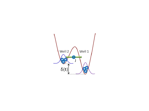
Figure 1: (Color online) Schematic diagram for BEC in a double-well potential where the time-dependent bias $\delta(t)$ is induced by an external field.

with the parameters

$$J = -\int dx[u_{1}^{\ast}(x)h_{0}u_{2}(x)],$$

$$\alpha = 2S_{0}\int dx[u_{1}^{\ast}(x)V_{1}(x)u_{1}(x)],$$

$$\delta_{1} = 2S_{1}\int dx[u_{1}^{\ast}(x)V_{1}(x)u_{1}(x)].$$

The term proportional to $J$ describes tunneling of particles from one to the other well, and we have assumed it to be real. In the same way, we stipulate that the overlap of the functions $u_{1}(x)$ and $u_{2}(x)$ be only minute, which implies that the condensates in the two wells are merely weakly coupled, and ignore the high-order overlaps between two functions martin ; gati2007 ; Lee2012 . Then the interaction between atoms $H_{int}$ is given as

$$H_{int}=\frac{U_{11}}{4}\hat{a}_{1}^{\dagger}\hat{a}_{1}^{\dagger}\hat{a}_{1}\hat{a}_{1}+\frac{U_{22}}{4}\hat{a}_{2}^{\dagger}\hat{a}_{2}^{\dagger}\hat{a}_{2}\hat{a}_{2},$$ (5)

with

$$U_{jj}=2g\int dx|u_{j}(x)|^{4},\ \ j=1,2.$$

After omitting the constant terms $O(N)$ and $O(N^{2})$, the total Hamiltonian now can be rewritten as a two-mode Bose-Hubbard Hamiltonian

$$H(t) = -J(\hat{a}_{1}^{\dagger}\hat{a}_{2}+\hat{a}_{2}^{\dagger}\hat{a}_{1})+\frac{E_{c}}{8}(\hat{a}_{2}^{\dagger}\hat{a}_{2}-\hat{a}_{1}^{\dagger}\hat{a}_{1})^{2}$$ (6)

$$+ \frac{\delta(t)}{2}(\hat{a}_{2}^{\dagger}\hat{a}_{2}-\hat{a}_{1}^{\dagger}\hat{a}_{1}),$$

with $E_{c}=U_{11}+U_{22}$ and time-dependent energy bias

$$\delta(t)=\alpha t+\delta_{1}\cos(\omega t).$$ (7)

In addition, by introducing the angular momentum operators $S_{x}=(\hat{a}_{1}^{\dagger}\hat{a}_{2}+\hat{a}_{1}\hat{a}_{2}^{\dagger})/2$, $S_{y}=(\hat{a}_{2}^{\dagger}\hat{a}_{1}-\hat{a}_{1}^{\dagger}\hat{a}_{2})/2i$, and $S_{z}=(\hat{a}_{2}^{\dagger}\hat{a}_{2}-\hat{a}_{1}^{\dagger}\hat{a}_{1})/2$ with the Casimir invariant

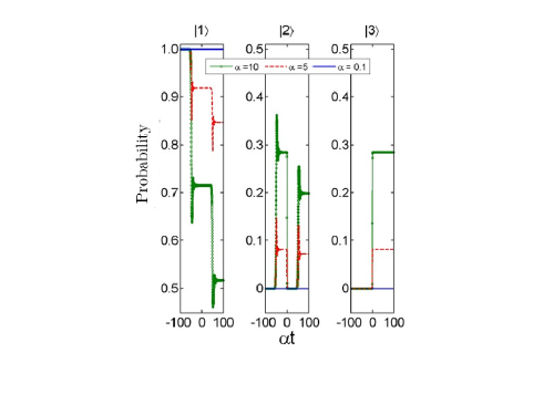
Figure 2: (Color online) Occupation probability of the system in the instantaneous eigenstates of the Hamiltonian $H(t)_{\delta_{1}=0}$ for three different values of the sweep rate $\alpha$ with $N=2$, $J=1$, $E_{c}=100$, and $\delta_{1}=0$. The system initially starts from its instantaneous ground state with a large negative bias. Here the solid lines are for $\alpha=0.1$, the dashed lines are for $\alpha=5$, and the solid lines with circles are for $\alpha=10$. Here the labels $|1\rangle,|2\rangle$, and $|3\rangle$ represent the three lowest instantaneous eigenstates of the Hamiltonian $H(t)_{\delta_{1}=0}$.

$S^{2}=(N/2)(N/2+1)$, the Hamiltonian (6) also can be rewritten as

$$H(t)=-2JS_{x}+\frac{E_{c}}{2}S_{z}^{2}+\delta(t)S_{z}.$$ (8)

Clearly, the problem with $\delta_{1}=0$ is reduced to the usual many-body LZ problem korsch . We note that in the mean-field approximation where the system can be described by a nonlinear two-level model, the nonlinear LZ process in a periodic driving field has been studied qzhang .

III Photon-induced sideband transitions

In the following, we discuss the effect of the additional periodic driving on the many-body LZ tunneling process. By expanding the state vector $|\psi(t)\rangle$ as a liner combination of the Fock states $|N/2-n,N/2+n\rangle$, denoting the state with $N/2-n$ bosons on the first well and $N/2+n$ on the second well,

$$|\psi(t)\rangle=\sum_{n=-N/2}^{N/2}\exp[-i\theta_{n}(t)]c_{n}(t)|N/2-n,N/2+n\rangle,$$

with

$$\theta_{n}(t) = \int_{0}^{t}[E_{c}n^{2}/2+(\alpha\tau+\delta_{1}\cos(\omega\tau))n]d\tau$$

$$= E_{c}n^{2}t/2+\alpha nt^{2}/2+\delta_{1}n\sin(\omega t)/\omega,$$

from the time-dependent Schrödinger equation $i\partial|\psi(t)\rangle/\partial t=H(t)|\psi(t)\rangle$, we can get $N+1$ coupled first-order differential equations for the coefficients $c_{n}(t)$

$$i\frac{dc_{n}}{dt}= -J\sqrt{(\frac{N}{2}-n)(\frac{N}{2}+n+1)}e^{-i\Delta\theta_{n+1}^{n}}c_{n+1}$$ (9)

$$-J\sqrt{(\frac{N}{2}+n)(\frac{N}{2}-n+1)}e^{i\Delta\theta_{n}^{n-1}}c_{n-1},$$

with $\Delta\theta_{n+1}^{n}=\theta_{n+1}-\theta_{n}=E_{c}(2n+1)t/2+\alpha t^{2}/2+\delta_{1}\sin(\omega t)/\omega$. By applying the generating function of the Bessel functions, $\exp[\pm i\delta_{1}\sin(\omega t)/\omega]=\sum_{m=-\infty}^{\infty}J_{m}(\delta_{1}/\omega)\exp[\pm im\omega t]$, we have

$$i\frac{dc_{n}}{dt}= -\sum_{m=-\infty}^{\infty}\widetilde{J}_{n,eff}^{m}e^{-i\varphi_{n}^{m}}c_{n+1}$$ (10)

$$-\sum_{m=-\infty}^{\infty}\widetilde{J}_{n-1,eff}^{m}e^{i\varphi_{n-1}^{m}}c_{n-1},$$

with

$$\widetilde{J}_{n,eff}^{m} = J\sqrt{(\frac{N}{2}-n)(\frac{N}{2}+n+1)}J_{m}(\delta_{1}/\omega),$$ (11)

$$\varphi_{n}^{m} = E_{c}(2n+1)t/2+\alpha t^{2}/2+m\omega t.$$ (12)

In our study, we mainly focus on the strong interaction regime where the interaction energy $E_{c}$ dominates the tunneling coupling $E_{c}/J>>1$ Lee ; Chena ; Kasztelan and the high-frequency limit $E_{c}/J>>\omega/J>>1$. Therefore, these terms on the right hand side of Eq. (10) are rapidly oscillating, and make important contributions only if $\varphi_{n}^{m}$ has a stationary phase at certain instant determined by the following condition Kayanuma ; Ful

$$\frac{d\varphi_{n}^{m}}{dt}=E_{c}(2n+1)/2+\alpha t+m\omega,$$ (13)

thereby resulting in

$$\alpha t_{n}^{m}=-(n+1/2)E_{c}-m\omega.$$ (14)

In the absence of the periodic driving field, $\delta_{1}=0$, the last term $m\omega$ vanishes. We note that in the case of $\delta_{1}=0$, the ground state undergoes $N$ LZ transitions at $\alpha t_{n}=-(n+1/2)E_{c}$. So the LZ transitions at $t_{n}^{0}=t_{n}$ just correspond to the usual many-body LZ process without periodic driving. Naturally, a problem arises, what is the dynamics of the system near $t_{n}^{m}$ with $m\neq 0$?

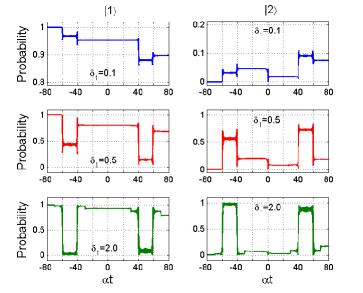
Figure 3: (Color online) Occupation probability of the system in the two lowest instantaneous eigenstates of the Hamiltonian $H(t)_{\delta_{1}=0}$ for different driving amplitudes $\delta_{1}$ with $N=2$, $J=1$, $E_{c}=100$, $\alpha=0.01$, and $\omega=10$. Here the labels $|1\rangle$ and $|2\rangle$ represent the two lowest instantaneous eigenstates of the Hamiltonian $H(t)_{\delta_{1}=0}$.

To answer this problem, we first make a change of variable $\tau=t-t_{n}^{m}$ near $t_{n}^{m}$, and then assume a high-frequency driving $\omega/J>>1$ for simplifying our discussions. Because of $\omega/J>>1$, we may retain the $m$-th term, and approximately replace the Eq. (10) by two first-order differential equations Kayanuma ; Ful

$$i\frac{dc_{n}}{d\tau} = -\widetilde{J}_{n,eff}^{m}e^{-i\phi_{n}^{m}}e^{-i\frac{\alpha\tau^{2}}{2}}c_{n+1},$$ (15)

$$i\frac{dc_{n+1}}{d\tau} = -\widetilde{J}_{n,eff}^{m}e^{i\phi_{n}^{m}}e^{i\frac{\alpha\tau^{2}}{2}}c_{n},$$ (16)

where $\phi_{n}^{m}=\alpha(t_{n}^{m})^{2}/2+E_{c}(2n+1)t_{n}^{m}/2+m\omega t_{n}^{m}$. Here $n$ takes from $-N/2$ to $N/2-1$. We note that similar coupled equation between $c_{n}$ and $c_{n-1}$ can also be obtained where $n$ starts from $N/2$ to $-N/2+1$.

To clearly see the physics described by the above equations, we make the transformation $c_{n}=\widetilde{c}_{n}\exp[-i\alpha\tau^{2}/4]$ and $c_{n+1}=\widetilde{c}_{n+1}\exp[i\alpha\tau^{2}/4]$, and get

$$i\frac{d\widetilde{c}_{n}}{d\tau} = -\frac{\alpha\tau}{2}\widetilde{c}_{n}-\widetilde{J}_{n,eff}^{m}e^{-i\phi_{n}^{m}}\widetilde{c}_{n+1},$$ (17)

$$i\frac{d\widetilde{c}_{n+1}}{d\tau} = \frac{\alpha\tau}{2}\widetilde{c}_{n+1}-\widetilde{J}_{n,eff}^{m}e^{i\phi_{n}^{m}}\widetilde{c}_{n}.$$ (18)

These results tell us that the change of the coefficients $c_{n}$ due to a linear sweep across $t=t_{n}^{m}$ is nothing but that of the LZ-type level crossing in which the coupling is renormalized effectively by a factor of the Bessel function.

Therefore, the LZ transitions at $\alpha t_{n}^{0}$ just correspond to the usual LZ transitions without a periodic driving field, while the sideband LZ transitions at $\alpha t_{n}^{m}$ with $m\neq 0$ arise from the periodic driving field of the time-dependent bias. In principle, the index $m$ can take arbitrary integer values. However, from the well-know fact that $J_{m}(\delta_{1}/\omega)\rightarrow 0$ with $m\neq 0$ if $\delta_{1}/\omega\rightarrow 0$ or $m\rightarrow\pm\infty$, it follows that for the very small driving amplitude, the sideband LZ transitions are so small that they are actually not visible. If the driving amplitude is chosen suitably, they become important and visible.

To confirm our analytical results with numerical simulations, we use the usual many-body LZ Hamiltonian $H(t)_{\delta_{1}=0}$ as a reference system. We solve numerically the time-dependent Schrödinger equation $i\partial|\psi(t)\rangle/\partial t=H(t)|\psi(t)\rangle$ starting from the ground state of Hamiltonian (6) with a large negative bias $\delta(t=-T)\rightarrow-\infty$, and at the end of the linear sweep $\delta(t=T)\rightarrow\infty$ of the bias, and compute the occupation probability of the system in the lowest instantaneous eigenstates of the Hamiltonian $H(t)_{\delta_{1}=0}$. In Fig. 2, we first display the numerical results without the periodic driving field for the small atom number $N=2$. Here the other parameters are given by $J=1$ and $E_{c}=100$. This situation corresponds to the usual many-body LZ problem. As is expected, if the sweep rate $\alpha$ is low enough, the system is still in the instantaneous ground state during the linear sweep. However, the presence of the periodic driving field modifies this physical picture. To only show the effect of the periodic driving, we take a small sweep rate $\alpha=0.01$, for which the evolution of the system without periodic driving field is adiabatic. In Fig. 3, we display the occupation probability of the system in the two lowest instantaneous eigenstates of the Hamiltonian $H(t)_{\delta_{1}=0}$ for different driving amplitudes with $N=2$, $J=1$, $\alpha=0.01$, $\omega=10$ and $E_{c}=100$. We find from these numerical results that the occupation probability displays a series of steplike changes at particular values of $\alpha t_{n}^{m}$ with $m\neq 0$. In this situation, for the small driving amplitudes $\delta_{1}=0.1$ and $\delta_{1}=0.5$, the LZ transitions with $m=\pm 1$ are clearly visible, while for a larger driving amplitudes $\delta_{1}=2.0$, the LZ transitions with $m=\pm 2$ become also visible.

IV Quantization of the periodic driving field

In this section, we show how to understand the sideband transitions in our many-body LZ process by quantizing the periodic driving field. Usually, the quantization of a classical field is achieved by introducing a harmonic oscillator and then quantizing the harmonic oscillator. We introduce a hybrid quantum-classical system composed of a quantum subsystem and a classical harmonic oscillator, and then show that the coupling between the quantum subsystem and the classical harmonic oscillator can act as the periodic driving for the quantum subsystem. Therefore, the quantization of the periodic driving field corresponds to the quantization of the classical harmonic oscillator in the hybrid quantum-classical system.

We consider a hybrid quantum-classical system

$$H_{hy}=H_{q}+H_{ho}+H_{q}^{ho},$$ (19)

with

$$H_{q}=-2JS_{x}+\frac{E_{c}}{2}S_{z}^{2}+\alpha tS_{z},$$ (20)

for the quantum subsystem,

$$H_{ho}=\frac{P^{2}}{2M}+\frac{1}{2}M\omega^{2}Q^{2}$$ (21)

for the classical harmonic oscillator, and

$$H_{q}^{ho}=kQS_{z},$$ (22)

for the coupling between the quantum subsystem and the classical harmonic oscillator. Here $k$ is the coupling strength, $Q$ is the oscillator position, and $P$ is the oscillator momentum. If the mass $M$ is large enough, the harmonic oscillator will not be affected by the quantum subsystem and the quantum subsystem feels a periodic driving produced by the harmonic oscillator makarov ; makri .

Through introducing the destruction and creation operators $b$ and $b^{\dagger}$ for the momentum $P$ and the position $Q$ of a harmonic oscillator, the fully quantum model for the hybrid quantum-classical system may be written as

$$H_{fq} = -2JS_{x}+\frac{E_{c}}{2}S_{z}^{2}+\alpha tS_{z}+\lambda(b^{\dagger}+b)S_{z}+\omega b^{\dagger}b.$$

Here $\lambda=k/\sqrt{2}$ is the rescaled coupling strength. For the case of $N=1$ and $E_{c}=0$, the resulting model can be used to describe the LZ process in a quantum two-level system coupled to a photon mode nori . By employing a unitary transformation $U=e^{i\omega tb^{\dagger}b}$, the quantum Hamiltonian (IV) is equivalent to an effective Hamiltonian

$$H_{fq}^{eff} = -2JS_{x}+\frac{E_{c}}{2}S_{z}^{2}+\alpha tS_{z}$$ (24)

$$+\lambda(e^{i\omega t}b^{\dagger}+e^{-i\omega t}b)S_{z}.$$

Clearly, if the harmonic oscillator stays in a coherent state $\left|\beta\right\rangle$, the quantum subsystem just feels a periodic driving field induced by the coupling term $H_{q}^{ho}$ and so that it obeys,

$$H_{q}^{eff} = -2JS_{x}+\frac{E_{c}}{2}S_{z}^{2}+\alpha tS_{z}$$ (25)

$$+\lambda\langle\beta|(e^{i\omega t}b^{\dagger}+e^{-i\omega t}b)|\beta\rangle S_{z},$$

$$= -2JS_{x}+\frac{E_{c}}{2}S_{z}^{2}+\alpha tS_{z}$$

$$+2\lambda\beta\cos(\omega t)S_{z}.$$

Usually, we can assume that $\beta$ is a real number. Then the amplitude of the periodic driving $\delta_{1}$ is related to $2\lambda\beta$.

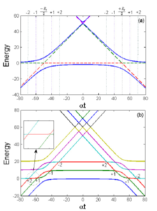
Figure 4: (Color online) (a) Instantaneous energy spectra of the many-body LZ Hamiltonian $H_{fq}$ for $J=0$ (dashed lines) and $J=1$ (solid liens) with $\lambda=\omega=0$. Here the total atom number is $N=2$, and the interaction strength is $E_{c}=100$. (b) Instantaneous energy spectra of the many-body LZ Hamiltonian $H_{fq}$ with $\lambda=1$ and $\omega=10$. Here for simplicity, we only take a relatively small basis set for the photon mode. The labels of -2,-1,+1 and +2 denote the avoided level-crossings at $\alpha t=\pm E_{c}/2-m\omega$ with $m=-2,-1,+1,+2$. In (b), the inset shows the enlarged region near the avoided level-crossings labeled by $m=+2,+1$.

To compute the energy spectrum of the Hamiltonian $H_{fq}$ with a fixed $\alpha t$, we use the basis $|n_{b}\rangle\otimes|n\rangle$ satisfying $b^{\dagger}b|n_{b}\rangle=n_{b}|n_{b}\rangle$ and $S_{z}|n\rangle=n|n\rangle$. For a small value of $\beta$, we may take a finite basis set, $n_{b}=0,1,2$, and diagonalize the Hamiltonian numerically. In Fig. 4, we display instantaneous energy spectra of the Hamiltonian $H_{fq}$ as a function of $\alpha t$ for two different cases (a) $\lambda=\omega=0$ and (b) $\lambda=1$ and $\omega=10$. In the two situations, the atom number is $N=2$, and the other parameters are given as $J=1$ and $E_{c}=100$. For the energy spectrum without the photon mode, the avoided level-crossings of the ground state only appear around $\alpha t=\pm E_{c}/2$ and these avoided level-crossings dominate the population transfer in the LZ process, as shown in Fig. 4 (a). For the energy spectrum in the presence of the photon mode, because of the many photon effects, the avoided level-crossings can appear around $\alpha t=\pm Ec/2-m\omega$ with $m=0,\pm 1,\pm 2$. It is observed that the gap around $\alpha t=\pm Ec/2-m\omega$ with $m=\pm 1$ is lager than those for $m=\pm 2$, as illustrated in Fig. 4 (b). This results explain why the sideband transitions with $m=\pm 1$ are observed in Fig. 3 for a relative small driving with $\delta_{1}=0.1,0.5$. When the driving amplitude is increased to a larger value related to a larger $\beta$, we need to include more photon numbers to compute the energy spectrum, and thus more sideband transitions may be observed. For example, in Fig. 3, the sideband transitions with $m=\pm 2$ are observed in the case of $\delta_{1}=2$.

V Conclusions

In summary, we have investigated the many-body LZ process in the two-site Bose-Hubbard model where the energy bias between sites is subject to a linear change with time and a periodic driving field. It is revealed that the periodic driving can modify the conditions for the many-body LZ transitions, and induce sideband LZ transitions under certain parameter conditions. In the high-frequency limit and strong interaction regime, we have applied an analytical method to understanding these sideband LZ transitions. In addition, by quantizing the periodic driving field, we introduce the fully quantum mechanical model to understand the sideband LZ transitions, in which the sideband transitions can be understood as the LZ transitions between states of different “photon” numbers. Our results show that the periodic driving field can provide an efficient way for controlling the many-body LZ tunneling process.

Our results of sideband transitions in many-body LZ problem offer an alternative route to manipulating many-body quantum systems. With currently avaliable experimental techniques for observing many-body LZ tunneling Chena , it is possible to test our theoretical predictions. It is also possible to apply our analysis for treating the case of more complex driving fields, such as multi- frequency driving field, and the driving field with time-dependent amplitude.

- (1) L. D. Landau, Phys. Z. Sowjetunion 2, 46 (1932).
- (2) C. Zener, Proc. R. Soc. London, Ser. A 137, 696 (1932).
- (3) E. C. G. Stüeckelberg, Helv. Phys. Acta 5, 369 (1932).
- (4) E. Majorana, Nuovo Cimento 9, 43 (1932).
- (5) Y. Qian, M. Gong, and C. Zhang, Phys. Rev. A 87, 013636 (2013).
- (6) S. Longhi and G. D. Valle, Phys. Rev. A 86, 043633 (2012).
- (7) C. Betthausen, T. Dollinger, H. Saarikoski, V. Kolkovsky, G. Karczewski, T. Wojtowicz, K. Richter, and D. Weiss, Science 337, 324 (2012).
- (8) W. D. Oliver, Y. Yu, J. C. Lee, K. K. Berggren, L. S. Levitov, and T. P. Orlando, Science 310, 1653 (2005).
- (9) B. Wu and Q. Niu, Phys. Rev. A 61, 023402 (2000).
- (10) O. Zobay and B. M. Garraway, Phys. Rev. A 61, 033603 (2000).
- (11) J. Liu, L. Fu, B. Ou, S. Chen, D. Choi, B. Wu, and Q. Niu, Phys. Rev. A 66, 023404 (2002).
- (12) D. Witthaut, E. M. Graefe, and H. J. Korsch, Phys. Rev. A 73, 063609 (2006).
- (13) A. Tomadin, R. Mannella, and S. Wimberger, Phys. Rev. A 77, 013606 (2008).
- (14) C. Lee, L.-B. Fu, and Y. S. Kivshar, Europhys. Lett. 81, 60006 (2008).
- (15) K. Smith-Mannschott, M. Chuchem, M. Hiller, T. Kottos, and D. Cohen, Phys. Rev. Lett. 102, 230401 (2009).
- (16) F. Trimborn, D. Witthaut, V. Kegel, and H. J. Korsch, New J. Phys. 12, 053010 (2010).
- (17) A. Zenesini, H. Lignier, G. Tayebirad, J. Radogostowicz, D. Ciampini, R. Mannella, S. Wimberger, O. Morsch, and E. Arimondo, Phys. Rev. Lett. 103, 090403 (2009).
- (18) C. Kasztelan, S. Trotzky, Y. Chen, I. Bloch, I. P. McCullöch, U. Schollwock, and G. Orso, Phys. Rev. Lett. 106, 155302 (2011).
- (19) M. Jona-Lasinio, O. Morsch, M. Cristiani, N. Malossi, J. H. Müller, E. Courtade, M. Anderlini, and E. Arimondo, Phys. Rev. Lett. 91, 230406 (2003).
- (20) T. Salger, C. Geckeler, S. Kling, and M. Weitz, Phys. Rev. Lett. 99, 190405 (2007).
- (21) S. Kling, T. Salger, C. Grossert, and M. Weitz, Phys. Rev. Lett. 105, 215301 (2010).
- (22) Y. Chen, S. Huber, S. Trotzky, I. Bloch, and E. Altman, Nature Physics 7, 61 (2011).
- (23) M. Grifoni and P. Hä nggi, Phys. Rep. 304, 229 (1998).
- (24) Y. Kayanuma and Y. Mizumoto, Phys. Rev. A 62, R061401 (2000).
- (25) S. Duan, L. Fu, J. Liu, and X. Zhao, Phys. Lett. A 346, 315 (2005).
- (26) N. Malossi, M. G. Bason, M. Viteau, E. Arimondo, R. Mannella, O. Morsch, and D. Ciampini, Phys. Rev. A 87, 012116 (2013).
- (27) M. Wubs, K. Saito, S. Kohler, Y. Kayanuma, and P. Hänggi, New J. Phys. 7, 218 (2005).
- (28) Q. Zhang, P. Hänggi, and J. Gong, New J. Phys. 10, 073008 (2008).
- (29) Q. Zhang, P. Hänggi, and J. Gong, Phys. Rev. A 77, 053607 (2008).
- (30) A. Smerzi, S. Fantoni, S. Giovanazzi, and S. R. Shenoy, Phys. Rev. Lett. 79, 4950 (1997).
- (31) G. J. Milburn, J. Corney, E. M. Wright, and D. F. Walls, Phys. Rev. A 55, 4318 (1997).
- (32) A. S. Parkins and D. F. Walls, Phys. Rep. 303, 1 (1998).
- (33) T. Jinasundera, C. Weiss, and M. Holthaus, Chemical Physics 322, 118 (2006).
- (34) R. Gati and M. K. Oberthaler, J. Phys. B 40, R61 (2007).
- (35) C. Lee, J. Huang, H. Deng, H. Dai, and J. Xu, Front. Phys. 7, 109 (2012).
- (36) G. Della Valle, M. Ornigotti, E. Cianci, V. Foglietti, P. Laporta, and S. Longhi, Phys. Rev. Lett. 98, 263601 (2007).
- (37) Y. V. Kartashov and V. A. Vysloukh, Opt. Lett. 34, 3544 (2009).
- (38) D. E. Makarov, Phys. Rev. E 48, R4146 (1993).
- (39) D. E. Makarov and N. Makri, Phys. Rev. E 52, 5863 (1995).
- (40) Z. Sun, J. Ma, X. Wang, and F. Nori, Phys. Rev. A 86, 012107 (2012).