Shortest reconfiguration paths in the solution space of Boolean formulas

Abstract

Given a Boolean formula and a satisfying assignment, a flip is an operation that changes the value of a variable in the assignment so that the resulting assignment remains satisfying. We study the problem of computing the shortest sequence of flips (if one exists) that transforms a given satisfying assignment $s$ to another satisfying assignment $t$ of a Boolean formula. Earlier work characterized the complexity of finding any (not necessarily the shortest) sequence of flips from one satisfying assignment to another using Schaefer’s framework for classification of Boolean formulas. We build on it to provide a trichotomy for the complexity of finding the shortest sequence of flips and show that it is either in P, NP-complete, or PSPACE-complete.

Our result adds to the small set of complexity results known for shortest reconfiguration sequence problems by providing an example where the shortest sequence can be found in polynomial time even though its length is not equal to the symmetric difference of the values of the variables in $s$ and $t$. This is in contrast to all reconfiguration problems studied so far, where polynomial time algorithms for computing the shortest path were known only for cases where the path modified the symmetric difference only.

1 Introduction

Reconfiguration problems study relationships between feasible solutions to an instance of a computational problem and have recently received significant attention [8, 20, 23, 26]. The relationship between solutions is typically analyzed with respect to a reconfiguration step, which specifies how one solution can be transformed into another.

For the problem of satisfiability, for example, one defines a reconfiguration step to be a flip operation, that is, changing the value of one variable in a satisfying assignment such that the resulting assignment is also satisfying. Most reconfiguration problems can be stated concisely in terms of a graph—the reconfiguration graph—that has a node for each feasible solution and an undirected edge between two solutions if either one can be formed from the other by a single reconfiguration step. Thus for the reconfiguration of satisfiability [19], there is a node for each satisfying assignment and an edge whenever the Hamming distance between two assignments, i.e. the number of variables in which the two assignments differ in value, is exactly one.

2 Background and motivation

2.0.1 Reconfiguration

In one of the earliest works on reconfiguration, Gopalan et al. [19] considered the problem of deciding if a sequence of flips exists that can reconfigure assignment $s$ to assignment $t$, both satisfying a Boolean formula $\phi$; they showed that for any class of formulas this question is either in P or is PSPACE-complete. Since then, reconfiguration versions of various problems have been studied, including maximum independent set, minimum vertex cover, maximum matching, shortest path, graph colorability, and many others [8, 20, 21, 22, 26]. Typical questions addressed in these works include the structure or the complexity of determining

• st-connectivity: whether there is a path from $s$ to $t$ in the reconfiguration graph [8, 20, 21, 22] or

• connectivity: whether the reconfiguration graph is connected [5, 11, 17] or

• upper bounds for the diameter of the reconfiguration graph [6, 8, 21].

More recently, there has been interest in finding shortest paths (if one exists) as well as in the parameterized complexity of reconfiguration problems [25, 26]. Although some algorithms for deciding st-connectivity also happen to compute the shortest path [20] (e.g. spanning trees, matchings), this is not the case for satisfiability of Boolean formulas, the subject of this paper. We study the question of computing the shortest flip sequence between two satisfying assignments and complementing Gopalan et al.’s work, provide a partition of the set of Boolean formulas into three equivalence classes where the problem is in P, NP-complete, or PSPACE-complete.

Reconfiguration problems exhibit several recurring patterns. For example, most reconfiguration versions of NP-complete decision problems are PSPACE-complete [8, 20] (e.g. maximum independent set) whereas versions of problems in P are in P [20] (e.g. maximum matching). Known exceptions include the shortest path and 3-coloring problems; the former is in P but has a reconfiguration version that is PSPACE-complete [7] and the latter is NP-complete but has a reconfiguration version that is in P [12]. Another recurring pattern is a connection between the st-connectivity problem (in P or PSPACE-complete) and the diameter of the reconfiguration graph (polynomial or exponential, respectively).

Most relevant to our work is the pattern that the only polynomial-time algorithms known for finding the shortest reconfiguration path have the property that they make no changes to parts of the solution common to $s$ and $t$. For trees and cactus graphs, the shortest path between maximum independent sets $s$ and $t$ never removes vertices in $s\cap t$ [25]. In the sequence of flips for 2CNF formulas (the only class for which a polynomial-time algorithm for shortest reconfiguration path of satisfiability was previously known), the only variables flipped are those whose values are different in $s$ and $t$ [19]. To the best of our knowledge, our results on computing the shortest path in a reconfiguration graph for satisfiability provide the first exception to this pattern. In particular, we provide a class of Boolean formulas where the shortest reconfiguration path can flip variables that have the same values in $s$ and $t$ and yet the path can be computed in polynomial time. Insights from our results may lead to a better understanding of the role of the symmetric difference in computing shortest reconfiguration paths.

2.0.2 Flips in triangulations

The problem of computing the shortest reconfiguration sequence has a long history in the field of triangulations [3, 10, 15, 24], although it has not been studied with this name. The reconfiguration of triangulations of a convex polygon makes use of a flip operation that replaces one diagonal with another. It is known that one can always transform one triangulation of a polygon to another [24]; therefore, research has focused on the complexity of finding shortest reconfiguration paths, where results have been obtained for planar point sets, simple polygons, convex polygons and triangulations where edges have labels [1, 9, 14, 28]. This problem is identical to reconfiguring independent sets for a certain kind of a graph, providing an example where although st-connectivity and connectivity are both trivially solvable, for many cases the complexity of shortest reconfiguration path has been open for more than 40 years [14].

Interestingly, one distinction between the case of convex polygons, which is open, and the case of simple polygons, which is NP-complete, is that the former but not the latter has the property that the shortest flip sequence never flips a diagonal shared by $s$ and $t$. This adds to the motivation for studying reconfiguration problems where the shortest reconfiguration path can be found in polynomial time even though the path flips objects that are already common between $s$ and $t$.

2.0.3 Reconfiguration on Boolean formulas and Schaefer’s framework

Schaefer’s [29] framework provides a way to classify Boolean formulas and was first used by Schaefer to show that for any class that can be defined using the framework, deciding whether a formula of that class has a satisfying assignment is either in P or NP-complete.

Schaefer’s framework has previously been used by Gopalan et al. [19] and Schwerdtfeger [30] in the context of reconfiguration, where they provide a similar characterization for st-connectivity and connectivity of the reconfiguration graph, respectively. In our work, we provide a similar complete characterization for finding the shortest reconfiguration path in terms of classes for which it is in P, NP-complete, or PSPACE-complete. In particular, our results imply that there are classes where we can compute shortest reconfiguration paths even when the path flips variables that have the same value in both $s$ and $t$.

2.0.4 Shortest paths in large graphs

A labelled hypercube in $n$ dimensions exhibits a shortest path finding algorithm that takes time logarithmic in the size of the graph—simply compute the Hamming distance between the two vertices. Partial cubes are subgraphs of the hypercube where the same property holds [16]. In general, a distance labeling scheme [18, 27, 31] is an assignment of bit vectors to the vertices of a given graph such that the length of the shortest path between two vertices can be computed just from the bit vectors assigned to the two vertices. Small distance labels provide efficient shortest path algorithms for large graphs.

Interestingly, the reconfiguration graph of satisfying assignments of 2CNF formulas is known to be a partial cube. One consequence of our results is the identification of a new class of subgraphs of the hypercube (reconfiguration graphs of navigable formulas, as defined in Section 3.1) where shortest paths can be found efficiently. Our class is fundamentally more complex than partial cubes in the sense that the distance between two vertices is not merely the Hamming distance between their labels.

3 Computing shortest reconfiguration paths

3.1 Preliminaries

We use terminology originally introduced by Schaefer [29] and adapted to reconfiguration by Gopalan et al. [19] and Schwerdtfeger [30].

A $k$-ary Boolean logical relation (or relation for short) $R$ is defined as a subset of $\{0,1\}^{k}$, where $k\geq 1$. Each $i\in\{1,\ldots,k\}$ can be interpreted as a variable of $R$ such that $R$ specifies exactly which assignments of values to the variables are to be considered satisfying.

For any $k$-ary relation $R$ and positive integer $k^{\prime}\leq k$, we define a $k^{\prime}$-ary restriction of $R$ to be any $k^{\prime}$-ary relation $R^{\prime}$ that can be obtained from $R$ by substitution with constants and identification of variables. More precisely, let $X:\{1,\ldots,k\}\rightarrow\{1,\ldots,k^{\prime}\}\cup\{c_{0},c_{1}\}$ be a mapping from the variables of $R$ to the variables of $R^{\prime}$ and the constants 0 and 1. Any such $X$ defines a mapping $f_{X}:\{0,1\}^{k^{\prime}}\rightarrow\{0,1\}^{k}$ as follows. For $r\in\{0,1\}^{k^{\prime}}$, let $f_{X}(r)$ be the $k$-bit vector whose $i^{th}$ bit is 0 if $X(i)=c_{0}$, 1 if $X(i)=c_{1}$ and equal to the $X(i)^{th}$ bit of $r$ otherwise. We say that a $k^{\prime}$-ary relation $R^{\prime}$ is a restriction of $R$ with respect to $X:\{1,\ldots,k\}\rightarrow\{1,\ldots,k^{\prime}\}\cup\{c_{0},c_{1}\}$ if $r\in R^{\prime}\Leftrightarrow f_{X}(r)\in R$.

A Boolean formula $\phi$ over a set $\{x_{1},\ldots,x_{n}\}$ of variables defines a relation $R_{\phi}$ as follows. For any $n$-bit vector $v\in\{0,1\}^{n}$, we interpret $v$ as the assignment to the variables of $\phi$ where $x_{i}$ is set to be equal to the $i^{th}$ bit of $v$. We then say that $v\in R_{\phi}$ if and only if $v$ is a satisfying assignment.

A CNF formula is a Boolean formula of the form $C_{1}\wedge\ldots\wedge C_{m}$, where each $C_{i}$, $1\leq i\leq m$, is a clause consisting of a finite disjunction of literals (variables or negated variables). A $k$CNF formula, $k\geq 1$, is a CNF formula where each clause has at most $k$ literals. A CNF formula is Horn (dual Horn) if each clause has at most one positive (negative) literal.

For a finite set of relations $\mathcal{S}$, a CNF($\mathcal{S}$) formula over a set of $n$ variables $\{x_{1},\ldots,x_{n}\}$ is a finite collection $\{C_{1},\ldots,C_{m}\}$ of clauses. Each $C_{i}$, $1\leq i\leq m$, is defined by a tuple $(R_{i},X_{i})$, where $R_{i}$ is a $k_{i}$-ary relation in $\mathcal{S}$ and $X_{i}:\{1,\ldots,k_{i}\}\rightarrow\{1,\ldots,n\}\cup\{c_{0},c_{1}\}$ is a function. Each $X_{i}$ defines a mapping $f_{X_{i}}:\{0,1\}^{n}\rightarrow\{0,1\}^{k_{i}}$ and we say that an assignment $v$ to the variables satisfies $\phi$ if and only if for all $i\in\{1,\ldots,m\}$, $f_{X_{i}}(v)\in R_{i}$. For any variable $x_{j}$, we say that $x_{j}$ appears in clause $C_{i}$ if $X_{i}(q)=j$ for some $q\in\{1,\ldots,k_{i}\}$ and for any assignment $v$ to the variables of $\phi$, we say that $f_{X_{i}}(v)$ is the assignment induced by $v$ on $R_{i}$.

For example, to represent the class 3CNF in Schaefer’s framework, we specify $\mathcal{S}$ as follows. Let $R^{0}=\{0,1\}^{3}\backslash\{000\}$, $R^{1}=\{0,1\}^{3}\backslash\{100\}$, $R^{2}=\{0,1\}^{3}\backslash\{110\}$, $R^{3}=\{0,1\}^{3}\backslash\{111\}$, and $\mathcal{S}=\{R^{0},R^{1},R^{2},R^{3}\}$. Since $R^{i}$ can be used to represent all 3-clauses with exactly $i$ negative literals (regardless of the positions in which they appear in a clause), clearly CNF($\mathcal{S}$) is exactly the class of 3CNF formulas.

Below we define some classes of relations used in the literature and relevant to our work. Note that componentwise bijunctive, OR-free and NAND-free were first defined by Gopalan et al. [19]. Schwerdtfeger [30] later modified them slightly and defined safely component-wise bijunctive, safely OR-free and safely NAND-free. We reuse the names componentwise bijunctive, OR-free and NAND-free for Schwerdtfeger’s safely component-wise bijunctive, safely OR-free and safely NAND-free respectively.

Definition 1

For a $k$-ary relation $R$:

• $R$ is bijunctive if it is the set of satisfying assignments of a 2CNF formula.

• $R$ is Horn (dual Horn) if it is the set of satisfying assignments of a Horn (dual Horn) formula.

• $R$ is affine if it is the set of satisfying assignments of a formula $x_{i_{1}}\oplus\ldots\oplus x_{i_{h}}\oplus c$, with $i_{1},\ldots,i_{h}\in\{1,\ldots,k\}$ and $c\in\{0,1\}$. Here $\oplus$ denote the exclusive OR operation which evaluates to $1$ when exactly one of the values it operates on is $1$ and evaluates to $0$ otherwise.

• $R$ is componentwise bijunctive if every connected component of the reconfiguration graph of $R$ and of the reconfiguration graph of every restriction $R^{\prime}$ of $R$ induces a bijunctive relation.

• $R$ is OR-free (NAND-free) if there does not exist a restriction $R^{\prime}$ of $R$ such that $R^{\prime}=\{01,10,11\}$ ($R^{\prime}=\{01,10,00\}$).

Using his framework, Schaefer showed that SAT($\mathcal{S}$)—the problem of deciding if a CNF($\mathcal{S}$) formula has a satisfying assignment—is in P if every relation in $\mathcal{S}$ is bijunctive, Horn, dual Horn, or affine, and is NP-complete otherwise. The result is remarkable because it divides a large set of problems into two equivalence classes based on their computational complexity, which is the opposite of what one might expect due to Ladner’s theorem [2].

Since Schaefer’s original paper, a myriad of problems about Boolean formulas have been analyzed, and similar divisions into equivalence classes obtained [13]. Gopalan et al.’s work [19], with corrections presented by Schwerdtfeger [30], shows a dichotomy for the problem of deciding whether a reconfiguration path exists between two satisfying assignments of a CNF($\mathcal{S}$) formula.

They call a set $\mathcal{S}$ of relations tight if

• all relations in $\mathcal{S}$ are componentwise bijunctive, or

• all relations in $\mathcal{S}$ are OR-free, or

• all relations in $\mathcal{S}$ are NAND-free.

They showed that the st-connectivity problem on CNF($\mathcal{S}$) formulas is in P if $\mathcal{S}$ is tight and PSPACE-complete otherwise.

Our trichotomy relies on a new class of formulas that subdivides the tight classes into those for which computing the shortest reconfiguration path can be done in polynomial time and those for which it is NP-complete.

Definition 2

For a $k$-ary relation $R$:

• $R$ is Horn-free if there does not exist a restriction $R^{\prime}$ of $R$ such that $R^{\prime}=\{0,1\}^{3}\setminus\{011\}$, or equivalently, $R^{\prime}$ is the set of all satisfying assignments of the clause $(x\vee\overline{y}\vee\overline{z})$ for some three variables $x$, $y$, and $z$.

• $R$ is dual-Horn-free if there does not exist a restriction $R^{\prime}$ of $R$ such that $R^{\prime}=\{0,1\}^{3}\setminus\{100\}$, or equivalently, $R^{\prime}$ is the set of all satisfying assignments of the clause $(\overline{x}\vee y\vee z)$ for some three variables $x$, $y$, and $z$.

The following is a useful observation.

Observation 1

For $k\geq 3$ and $R$ a $k$-ary relation, if $R$ is OR-free then it is dual-Horn-free. Similarly, if $R$ is NAND-free then it is Horn-free.

Proof

Assume that $R$ is OR-free but not dual-Horn-free. Then there exists a restriction $R^{\prime}$ of $R$ such that $R^{\prime}=\{0,1\}^{3}\setminus\{100\}$. It is easy to see that, from $R^{\prime}$, one can obtain $R^{\prime\prime}=\{01,10,11\}$ by setting one of the three variables in $R^{\prime}$ to $0$, resulting in a contradiction. A similar proof shows that NAND-free relations are Horn-free. ∎

Definition 3

We call a set $\mathcal{S}$ of relations navigable if one of the following holds:

• All relations in $\mathcal{S}$ are OR-free and Horn-free.

• All relations in $\mathcal{S}$ are NAND-free and dual-Horn-free.

• All relations in $\mathcal{S}$ are component-wise bijunctive.

It is clear that if $\mathcal{S}$ is navigable, then it is also tight. Our main result is the following trichotomy.

Theorem 3.1

For a CNF($\mathcal{S}$) formula $\phi$ and two satisfying assignments $s$ and $t$, the problem of computing the shortest reconfiguration path between $s$ and $t$ is in P if $\mathcal{S}$ is navigable, NP-complete if $\mathcal{S}$ is tight but not navigable and PSPACE-complete otherwise.

In the next section, we establish the hardness results; the rest of the paper is devoted to develop our polynomial time algorithm for navigable formulas. Interestingly, unlike previous classification results, while the NP-completeness result in our case turns out to be easier, the polynomial time algorithm is quite involved.

3.2 The hard cases

Gopalan et al. [19] showed that if $\mathcal{S}$ is not tight, then st-connectivity is PSPACE-complete for CNF($\mathcal{S}$). This implies that finding the shortest reconfiguration path is also PSPACE-complete for such classes of formulas.

Theorem 3.2

If $\mathcal{S}$ is tight but not navigable, then finding the shortest reconfiguration path on CNF($\mathcal{S}$) formulas is NP-complete.

Proof

The problem is in NP because the diameter of the reconfiguration graph is polynomial for all tight formulas, as shown by Gopalan et al. [19]. We now prove that it is, in fact, NP-complete.

As $\mathcal{S}$ is tight but not navigable, all relations in $\mathcal{S}$ are OR-free or all relations in $\mathcal{S}$ are NAND-free. Let us assume that all relations in $\mathcal{S}$ are NAND-free (we handle the other case later). Then, as $\mathcal{S}$ is not navigable, there exists a relation which is dual-Horn.

We show a reduction from Vertex Cover to such a CNF($\mathcal{S}$) formula. Given an instance $(G=(V,E),k)$ of Vertex Cover, we create a variable $x_{v}$ for each $v\in V$. For each edge $e=(u,v)\in E$, we create two new variables $y_{e}$ and $z_{e}$ and the clauses $(y_{e}\vee\overline{z_{e}}\vee x_{u})$ and $(z_{e}\vee\overline{y_{e}}\vee x_{v})$. The resulting formula $F(G)$ has $|V|+2|E|$ variables and $2|E|$ clauses.

It is easy to see that all the relations of $F(G)$ are NAND-free (as we cannot set the values of all but two of their variables to get a NAND relation), however none of them is dual-Horn-free (as each clause has two positive literals). Hence the formula $F(G)$ is tight but not navigable.

Let $s$ be the satisfying assignment for the formula with all variables set to $0$, and let $t$ be the satisfying assignment with all the variables $x_{v},v\in V$ set to $0$ and the rest set to $1$. If $G$ has a vertex cover $S$ of size at most $k$, then we can form a reconfiguration sequence of length at most $2|E|+2k$ from $s$ to $t$ by flipping each $x_{v},v\in S$ from $0$ to $1$, flipping the $y_{e}$ and $z_{e}$ variables, and then flipping each $x_{v},v\in S$ back from $1$ to $0$. To show that such a reconfiguration sequence exists only if there exists such a vertex cover, we observe that if neither $x_{u}$ nor $x_{v}$ has been flipped to 1, neither $y_{e}$ nor $z_{e}$ can be flipped to 1 while keeping the formula satisfied at the intermediate steps.

To show hardness when all relations in $\mathcal{S}$ are OR-free but not Horn-free, we give a reduction from Independent set. Given $G=(V,E)$ and an integer $k$, we create, as before, a variable $x_{v}$ for each $v\in V$ and two variables $y_{e}$ and $z_{e}$ for each $e\in E$. For each edge $e=(u,v)\in E$, we create the clauses $(y_{e}\vee\overline{z_{e}}\vee\overline{x_{u}})$ and $(\overline{y_{e}}\vee z_{e}\vee\overline{x_{v}})$. Clearly, all the relations of the formula are OR-free, and none of them is Horn-free.

We let $s$ be the satisfying assignment that sets all the variables to $1$, and $t$ be the satisfying assignment that sets all the variables to $0$ except the variables $x_{v}v\in V$ that are set to $1$. If $G$ has an independent set of size at least $k$, then it has a vertex cover $S$ of size at most $n-k$, then we can form a reconfiguration sequence of length at most $2|E|+2(n-k)$ from $s$ to $t$ by flipping each $x_{v},v\in S$ from $1$ to $0$, flipping the $y_{e}$ and $z_{e}$ variables, and then flipping each $x_{v},v\in S$ back from $0$ to $1$. To show that such a reconfiguration sequence exists only if there exists such a vertex cover (of size $n-k$), we observe that if neither $x_{u}$ nor $x_{v}$ has been flipped to 0, neither $y_{e}$ nor $z_{e}$ can be flipped to 0 while keeping the formula satisfied at the intermediate steps. ∎

3.3 The polynomial-time algorithm for navigable formulas

In this section, we give the polynomial time algorithm to find the shortest reconfiguration sequence between two satisfying assignments of a navigable formula.

Gopalan et al. gave a polynomial-time algorithm for finding the shortest reconfiguration path in component-wise bijunctive formulas. The path, in this case, flips only variables that have different values in $s$ and $t$. The NP-completeness proof from the previous section crucially relies on the fact that we need to flip variables with common values; in fact, the hardness lies in deciding precisely which common variables need to be flipped. Thus it is tempting to conjecture that hardness for shortest reconfiguration path is caused by relations where the shortest distance is not always equal to the Hamming distance.

Interestingly, this intuition is wrong. The reconfiguration graph for the relation $R=\{000,001,101,111,110\}$ is a path of length four, where for 000 and 110 the shortest path is of length four but the Hamming distance is two. However, we can find shortest reconfiguration paths in formulas built out of $R$ in polynomial time, the exact reason for which will become clear in our general description of the algorithm. The intuitive reason is that there are very few candidates for shortest paths; if we restrict our attention to a single clause built out of $R$, then there exists a unique path to follow. It then suffices to determine whether there exist two clauses for which the prescribed paths are in conflict. In general, our proof relies on showing that even if there does not exist a unique path, the set of all possible paths between two satisfying assignments of a navigable formula is not diverse enough to make the problem computationally hard. We show that the set of all possible paths can be characterized using a partial order on the set of flips.

3.3.1 Notation

Our results make use of two different views of the problem (graph theoretic and algebraic), and hence two sets of notation.

The graph-theoretic view consists of the reconfiguration graph $G_{R}$ that has a node for each Boolean string $s\in R$ and an edge whenever the Hamming distance between the two strings is exactly one. We call a path from $s$ to $t$ monotonically increasing if the Hamming weights of the vertices on the path increase monotonically as we go from $s$ to $t$, and define a monotonically decreasing path similarly. A path is canonical if it consists of a monotonically increasing path followed by a monotonically decreasing path.

The algebraic view consists of a token system [16] consisting of a set $\mathscr{S}$ of states and a set $\tau$ of tokens. The tokens specify the rules of transition between states. Each token $t\in\tau$ is a function that maps $\mathscr{S}$ to itself. Given a $k$-ary relation $R$, we define a token system as follows. The set $\mathscr{S}$ of states consists of all the elements of $R$ and a special state $s^{*}$ called the invalid state that captures all the unsatisfying assignments of the formula. The set $\tau$ of tokens is the set $\{x_{1}^{+},\ldots,x_{k}^{+}\}\cup\{x_{1}^{-},\ldots,x_{k}^{-}\}$, where $x_{i}^{+}$ denotes a flip of variable $x_{i}$ from 0 to 1, which we call a positive flip, and denote the sign of the flip as positive, and $x_{i}^{-}$ denotes a flip of variable $x_{i}$ from 1 to 0, which we call a negative flip and denote the sign of the flip as negative.

To complete the description of the token system, we need to specify the function to which each token corresponds. For $x_{i}^{+}\in\tau$ and $s\in\mathscr{S}$, $x_{i}^{+}(s^{*})=s^{*}$, $x_{i}^{+}(s)=s^{*}$ if the value of variable $x_{i}$ in $s$ is 1, $x_{i}^{+}(s)=s^{\prime}$ if the value of variable $x_{i}$ in $s$ is 0 and the bit string $s^{\prime}$ obtained on flipping it to 1 lies in $R$, and $x_{i}^{+}(s)=s^{*}$ if the value of variable $x_{i}$ in $s$ is 0 and the bit string $s^{\prime}$ obtained on flipping it to 1 does not lie in $R$. The function $x_{i}^{-}$ is defined analogously. In the rest of this article, we will use the word “flip” instead of “token”, and we will use the words “state,” “vertex,” and “satisfying assignment” interchangeably.

A sequence of flips also defines a function, that is, the composition of all the functions in the sequence. We call a flip sequence invalid at a given state $s$ if the sequence applied to $s$ results in invalid state $s^{*}$, and valid otherwise. Two flip sequences are equivalent if they result in the same final state when applied to the same starting state. Finally, we call a flip sequence canonical if all positive flips in it occur before all the negative flips. That is, the path from its first state (node) to the last is a canonical path. Note that in any canonical flip sequence, each flip occurs at most once. Given two states $s,t\in{\mathscr{S}}$, we say that a set ${\mathscr{C}}$ of flips transforms $s$ to $t$ if the elements of ${\mathscr{C}}$ can be arranged in some order such that the resulting flip sequence transforms $s$ to $t$. For a given state $s$ and flip set ${\mathscr{C}}$, we say ${\mathscr{C}}$ is valid if the elements of ${\mathscr{C}}$ can be arranged in some order such that the resulting flip sequence applied to $s$ results in a valid state.

We describe a flip sequence simply by listing the flips in order. The flip sequence formed by removing flip $f$ from ${\mathcal{F}}$ is denoted ${\mathcal{F}}\setminus f$. The flip sequence obtained by reversing ${\mathcal{F}}$ is ${\mathcal{F}}^{-1}$, and by performing ${\mathcal{F}}_{1}$ followed by ${\mathcal{F}}_{2}$ is ${\mathcal{F}}_{1}\cdot{\mathcal{F}}_{2}$. We use ${\mathscr{C}}({\mathcal{F}})$ to denote the set of flips that appear in ${\mathcal{F}}$. A flip sequence (set) consisting of only positive flips will be called a positive flip sequence (set). We use ${\mathcal{F}}_{0}$ to denote an empty flip sequence and, by convention, define it to be valid. For a flip sequence ${\mathcal{F}}$, if $f\in{\mathcal{F}}$ appears before $f^{\prime}\in{\mathcal{F}}$ in the sequence, then we say $f<_{\mathcal{F}}f^{\prime}$. For a tuple $t=(x_{i_{1}},\ldots,x_{i_{d}})$ of variables and a state $s$, we use $s^{t}$ to denote the string of values restricted to $x_{i_{1}},\ldots,x_{i_{d}}$.

3.3.2 Overview of the algorithm

For a CNF($\mathcal{S}$) formula $\phi$ and two satisfying assignments $s$ and $t$, if every relation in $\mathcal{S}$ is componentwise bijunctive, then the algorithm of Gopalan et al. gives a polynomial time algorithm to find a shortest path between $s$ and $t$. Hence we will assume that every relation in $\phi$ is NAND-free and dual-Horn-free.

There are two crucial properties of NAND-free and dual-Horn-free relations that help us design a polynomial time algorithm. First, we show in Lemma 2 (originally proved by Gopalan et al.) that in a NAND-free relation, any valid flip sequence from $s$ to $t$ can be transformed into an equivalent canonical flip sequence, where all positive flips are performed before all negative flips. Since the vertex reached after performing all the positive flips has a larger Hamming weight than both $s$ and $t$, it can be viewed as a common ancestor, and thus the shortest reconfiguration sequence defines a “least common ancestor”. Note however that finding such a least common ancestor may not be easy, as not all orderings of those positive flips may be valid.

Next, we show that if the relation is both NAND-free and dual-Horn-free, then the set of positive valid flip sets starting from a given satisfying assignment $s$ forms a distributive lattice [4]. Thus using Birkhoff’s representation theorem [4], we obtain a partial order among the positive flips that any valid flip sequence must follow. Moreover, since the positive valid flip sets have a lattice structure, $s$ and $t$ have a unique least common ancestor. We use the partial order to find it.

If every relation in $\mathcal{S}$ is OR-free and Horn-free, similar properties hold but the role of positive and negative flips is “reversed”. In other words, in an OR-free relation, any valid flip sequence from $s$ to $t$ can be transformed into an equivalent flip sequence, where all negative flips are performed before all positive flips. Moreover, if the relation is both OR-free and Horn-free, the set of negative flips becomes characterizable by a partial order. Hence, we will only consider properties of NAND-free and dual-Horn-free relations. Our algorithm for NAND-free and dual-Horn-free relations can easily be modified to handle OR-free and Horn-free relations.

3.3.3 The token system of NAND-free relations

We begin by proving some useful properties of the token system formed by NAND-free relations.

Lemma 1

For $R$ a NAND-free relation and ${\mathcal{F}}=f_{1}\ldots f_{q}$ a valid flip sequence at $s\in R$, if there exists $i\in\{1,\ldots,q-1\}$ such that $f_{i}=x^{-}$ is a negative flip and $f_{i+1}=y^{+}$ is a positive flip, with $x\neq y$, then the sequence ${\mathcal{F}}^{\prime}=f_{1}\ldots f_{i-1}f_{i+1}f_{i}\ldots f_{q}$ is also valid at $s$ and is equivalent to ${\mathcal{F}}$, i.e., swapping $f_{i}$ and $f_{i+1}$ results in an equivalent flip sequence.

Proof

Let $u$ be the state right before applying $f_{i}$ in ${\mathcal{F}}$, $v=f_{i}(u)$ be the state after applying $f_{i}$ but before applying $f_{i+1}$, and $w=f_{i+1}(v)$ be the one after applying $f_{i+1}$. Thus it is clear that $u^{(x,y)}=10,v^{(x,y)}=00$, and $w^{(x,y)}=01$. Also, notice that since no other variables are flipped between $u,v$, and $w$, the values of all variables other than $x$ and $y$ remain the same in the states $u$, $v$ and $w$. Let $t$ be the Boolean string whose value is the same as $u,v$, and $w$ on all variables except $x$ and $y$ and $t^{(x,y)}=11$. If $t\notin R$, then the substitution described above gives us the relation $\{10,00,01\}$ on $x$ and $y$, which is precisely the NAND relation. Since $R$ is NAND-free, $t\in R$ (Figure 1 (a)) and thus we can replace the path $u\rightarrow v\rightarrow w$ with the path $u\rightarrow t\rightarrow w$. This is equivalent to swapping the flips $f_{i+1}$ and $f_{i}$. ∎

Lemma 2 now follows immediately. It shows (first proved by Gopalan et al. [19]) that any valid flip sequence can be made canonical.

Lemma 2

For $R$ a NAND-free relation, if ${\mathcal{F}}$ is a valid sequence at $s\in R$, then there exists a valid canonical sequence ${\mathcal{F}}^{\prime}$ equivalent to ${\mathcal{F}}$ such that ${\mathscr{C}}({\mathcal{F}}^{\prime})\subseteq{\mathscr{C}}({\mathcal{F}})$ and, for any two flips $f_{1},f_{2}\in{\mathcal{F}}^{\prime}$ of the same sign, if $f_{1}<_{{\mathcal{F}}^{\prime}}f_{2}$ then $f_{1}<_{{\mathcal{F}}}f_{2}$, i.e., the relative order among flips of the same sign is preserved.

Proof

If ${\mathcal{F}}$ is not canonical, it must have a negative flip followed by a positive flip somewhere. If both flips act on the same variable, we cancel them out; otherwise, we swap them using the proof of Lemma 1. Doing this repeatedly gives us the required canonical sequence ${\mathcal{F}}^{\prime}$. The order among the flips of the same sign is preserved since we never swap two flips of the same sign.∎

Lemma 3

For $R$ a NAND-free relation, if ${\mathscr{C}}_{1}$ and ${\mathscr{C}}_{2}$ are two positive flip sets that are valid at $s\in R$, then ${\mathscr{C}}_{1}\cup{\mathscr{C}}_{2}$ is also a valid flip set at $s$.

Proof

Let $u={\mathcal{F}}_{1}(s)$ and $v={\mathcal{F}}_{2}(s)$, where ${\mathcal{F}}_{1}$ and ${\mathcal{F}}_{2}$ are valid flip sequences such that ${\mathscr{C}}(F_{1})={\mathscr{C}}_{1}$ and ${\mathscr{C}}(F_{2})={\mathscr{C}}_{2}$. Clearly, ${\mathcal{F}}_{1}^{-1}\cdot{\mathcal{F}}_{2}$ is a valid flip sequence from $u$ to $v$. Thus, we can apply Lemma 2 to the sequence ${\mathcal{F}}_{1}^{-1}\cdot{\mathcal{F}}_{2}$ to transform it into the canonical sequence ${\mathcal{F}}$. Let ${\mathcal{F}}^{+}$ denote the prefix of ${\mathcal{F}}$ that contains all the positive flips. It is clear that ${\mathcal{F}}_{1}\cdot{\mathcal{F}}^{+}$ is a valid flip sequence at $s$ and ${\mathscr{C}}({\mathcal{F}}_{1}\cdot{\mathcal{F}}^{+})={\mathscr{C}}_{1}\cup{\mathscr{C}}_{2}$. ∎

Later, we prove a similar lemma for the intersection of two flip sets, but for dual-Horn-free relations. We conclude this subsection with a lemma that shows that if two disjoint flips sets are valid at a state, we can, in some sense, perform them (the two sets of flips) one after the other in either order.

Lemma 4

For $R$ a NAND-free relation and ${\mathcal{F}}_{1}$ and ${\mathcal{F}}_{2}$ two positive flip sequences that are valid at $s\in R$, if ${\mathscr{C}}({\mathcal{F}}_{1})\cap{\mathscr{C}}({\mathcal{F}}_{2})=\emptyset$, then ${\mathcal{F}}_{1}$ is valid at ${\mathcal{F}}_{2}(s)$ and ${\mathcal{F}}_{2}$ is valid at ${\mathcal{F}}_{1}(s)$.

Proof

Consider the sequence ${\mathcal{F}}_{2}^{-1}\cdot{\mathcal{F}}_{1}$ that transforms ${\mathcal{F}}_{2}(s)$ to ${\mathcal{F}}_{1}(s)$. Applying Lemma 2 to it, we obtain the canonical flip sequence ${\mathcal{F}}_{1}\cdot{\mathcal{F}}_{2}^{-1}$. Thus ${\mathcal{F}}_{1}$ is valid at ${\mathcal{F}}_{2}(s)$. Using the same argument on the sequence ${\mathcal{F}}_{1}^{-1}\cdot{\mathcal{F}}_{2}$ proves the other claim. ∎

3.3.4 The token system of dual-Horn-free relations

In this section, we establish stronger properties with the assumption that $R$ is not only NAND-free, but is also dual-Horn-free. We begin by establishing a simple property of relations that are NAND-free and dual-Horn-free in the following lemma.

Lemma 5

Let $R$ be a NAND-free and dual-Horn-free relation and $s,t_{1},t_{2}\in R$ be three distinct states such that the flip sequence ${\mathcal{F}}_{1}=x_{k}^{+}x_{i}^{+}$ transforms $s$ to $t_{1}$, the flip sequence ${\mathcal{F}}_{2}=x_{j}^{+}x_{i}^{+}$ transforms $s$ to $t_{2}$, and $x_{k}\neq x_{j}$. Then the sequence ${\mathcal{F}}_{1}^{\prime}=x_{i}^{+}x_{k}^{+}$ also transforms $s$ to $t_{1}$ and the sequence ${\mathcal{F}}_{2}^{\prime}=x_{i}^{+}x_{j}^{+}$ also transforms $s$ to $t_{2}$, i.e., we can swap the flips in both ${\mathcal{F}}_{1}$ and ${\mathcal{F}}_{2}$.

Proof

For $u_{1}=x_{k}^{+}(s)$ and $u_{2}=x_{j}^{+}(s)$, the sequence $x_{j}^{-}x_{k}^{+}$ transforms $u_{2}$ to $u_{1}$. We can reorder the sequence to obtain $x_{k}^{+}x_{j}^{-}$, using Lemma 1. For $v=x_{k}^{+}(u_{2})$, we can use a similar argument to show that $x_{i}^{+}$ is a valid flip at $v$; we let $w=x_{i}^{+}(v)$. The values of variables $x_{i}$, $x_{j}$, and $x_{k}$ at states $s,u_{1},u_{2},t_{1},t_{2},v$, and $w$ form exactly the seven satisfying assignments $\{000,001,010,101,110,011,111\}$ of the dual-Horn clause $(\overline{x_{i}}\vee x_{j}\vee x_{k})$ (Figure 1 (b)). But since $R$ is dual-Horn-free, there must also exist the state $v^{\prime}$ for which $x_{i}=1,x_{j}=0,x_{k}=0$. The path $s\rightarrow v^{\prime}\rightarrow t_{1}$ gives the sequence $x_{i}^{+}x_{k}^{+}$ and the path $s\rightarrow v^{\prime}\rightarrow t_{2}$ gives the sequence $x_{i}^{+}x_{j}^{+}$. ∎

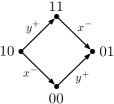
(a)

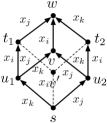
(b)

Figure 1: (a) Example for Lemma 1 (b) Example for Lemma 5

The seemingly innocuous lemma above turns out to be very powerful. In the following sequence of lemmas, we cleverly build on top of it to eventually prove that the set of all positive valid flip sets starting from an assignment $s$ forms a distributive lattice. The lattice structure then helps us formulate a polynomial time algorithm for computing the shortest reconfiguration path.

Lemma 6

Let $R$ be a NAND-free and dual-Horn-free relation and $s,t\in R$ be two satisfying assignments such that $x^{+}y^{+}$ is a valid flip sequence at $s$ and $y^{+}$ is a valid flip at $t$. Furthermore, let ${\mathcal{F}}$ be a positive flip sequence such that ${\mathcal{F}}(s)=t$ and $x^{+}\not\in{\mathscr{C}}({\mathcal{F}})$. Then, the sequence $y^{+}x^{+}$ must also be valid at $s$.

Proof

Let $v$ be the vertex with smallest Hamming weight on the path corresponding to ${\mathcal{F}}$ from $s$ to $t$ (including $s$ and $t$) at which $y^{+}$ is a valid flip. Let ${\mathcal{F}}_{1}=x^{+}y^{+}$ and let ${\mathcal{F}}_{2}$ be the positive flip sequence that transforms $s$ to $v$, i.e. $v={\mathcal{F}}_{2}(s)$. Note that ${\mathscr{C}}({\mathcal{F}}_{1})\cap{\mathscr{C}}({\mathcal{F}}_{2})=\emptyset$, as neither $x^{+}$ nor $y^{+}$ can appear in ${\mathscr{C}}({\mathcal{F}}_{2})$ (See Figure 2(a)). If $v=s$, we are done; then let us assume this not to be the case. Let $u$ be the vertex immediately before $v$ on the path from $s$ to $t$ and let $z^{+}(u)=v$. Since ${\mathscr{C}}({\mathcal{F}}_{1})\cap{\mathscr{C}}({\mathcal{F}}_{2})=\emptyset$ and ${\mathscr{C}}({\mathcal{F}}_{1})\cap\{{\mathscr{C}}({\mathcal{F}}_{2})\setminus\{z^{+}\}\}=\emptyset$, we can apply Lemma 4 at $s$, which implies that $x^{+}y^{+}$ must be valid at both $u$ and $v$. Now we use Lemma 5 at $u$. Since both $x^{+}y^{+}$ and $z^{+}y^{+}$ are valid sequences at $u$, $y^{+}x^{+}$ must also be a valid sequence at $u$. This contradicts the assumption that $v$ was the vertex with smallest Hamming weight on the path where $y^{+}$ was a valid flip. ∎

Lemma 7

For $R$ a NAND-free and dual-Horn-free relation, if ${\mathcal{F}}_{1}\cdot x^{+}\cdot y^{+}$ and ${\mathcal{F}}_{2}\cdot y^{+}$ are both valid positive flip sequences at $s\in R$ such that $x^{+}\not\in{\mathscr{C}}({\mathcal{F}}_{2})$ then ${\mathcal{F}}_{1}\cdot y^{+}\cdot x^{+}$ is also valid at $s$.

Proof

Let $u={\mathcal{F}}_{1}(s)$ and $v={\mathcal{F}}_{2}(s)$. We apply Lemma 2 to the sequence ${\mathcal{F}}_{1}^{-1}\cdot{\mathcal{F}}_{2}$ that transforms $u$ to $v$ to obtain the canonical sequence ${\mathcal{F}}={\mathcal{F}}^{+}\cdot{\mathcal{F}}^{-}$. Let $w$ be the vertex with maximum Hamming weight on this canonical path (Figure 2(b)). Hence, we have $w={\mathcal{F}}^{+}(u)$ and $v={\mathcal{F}}^{-}(w)$. Note that ${\mathcal{F}}$ does not involve flips of the variables $x$ or $y$.

Since $y^{+}$ is a valid flip at $v$, $y^{+}\not\in{\mathscr{C}}({\mathcal{F}}^{-})$, and the path from $v$ to $w$ is monotonically increasing, from Lemma 4, $y^{+}$ is also valid at $w$. Now using Lemma 6, since $x^{+}y^{+}$ is valid at $u$, $x^{+}\not\in{\mathcal{F}}^{+}$, and $y^{+}$ is valid at $w$, we have that $y^{+}x^{+}$ is also valid at $u$. ∎

(a)

(b)

Figure 2: Dotted lines denote paths and solid lines denote edges. Hamming weight increases in the upward direction. (a) Proof of Lemma 6 (b) Proof of Lemma 7.

Lemma 3 already shows that the set of valid flip sets is closed under union. To prove that the set of valid flip sets forms a distributive lattice, we need to show that it is also closed under intersection, which we do in the next lemma.

Lemma 8

For $R$ a NAND-free and dual-Horn-free relation, if ${\mathscr{C}}_{1}$ and ${\mathscr{C}}_{2}$ are two positive flip sets that are valid at $s\in R$, then ${\mathscr{C}}_{1}\cap{\mathscr{C}}_{2}$ is also a valid flip set at $s$.

Proof

If ${\mathscr{C}}_{1}\subseteq{\mathscr{C}}_{2}$ or ${\mathscr{C}}_{2}\subseteq{\mathscr{C}}_{1}$, then the statement is trivial. Otherwise, consider any valid ordering ${\mathcal{F}}_{1}$ of ${\mathscr{C}}_{1}$. We show that if $x^{+}$ and $y^{+}$ are two consecutive elements of ${\mathcal{F}}_{1}$ such that $x^{+}\in{\mathscr{C}}_{1}\backslash{\mathscr{C}}_{2}$, $y^{+}\in{\mathscr{C}}_{1}\cap{\mathscr{C}}_{2}$ and $x^{+}<_{{\mathcal{F}}_{1}}y^{+}$, then swapping $x^{+}$ and $y^{+}$ also gives a valid ordering of ${\mathscr{C}}_{1}$. Applying such swaps repeatedly, we get an ordering where all elements of ${\mathscr{C}}_{1}\cap{\mathscr{C}}_{2}$ appear before all elements of ${\mathscr{C}}_{1}\backslash{\mathscr{C}}_{2}$ thus proving that ${\mathscr{C}}_{1}\cap{\mathscr{C}}_{2}$ is a valid set at $s$.

To see how to swap $x^{+}$ and $y^{+}$ in ${\mathcal{F}}_{1}$, suppose $u$ is the vertex on the path corresponding to ${\mathcal{F}}_{1}$ on which the sequence $x^{+}\cdot y^{+}$ is performed, and consider an arbitrary valid ordering ${\mathcal{F}}_{2}$ of ${\mathscr{C}}_{2}$. Let $v$ be the vertex on the path corresponding to ${\mathcal{F}}_{2}$ on which $y^{+}$ is performed. Such a vertex exists since $y^{+}\in{\mathscr{C}}_{1}\cap{\mathscr{C}}_{2}$. Now, since $x^{+}\cdot y^{+}$ is valid at $u$, $y^{+}$ is valid at $v$ and the monotonically increasing path from $s$ to $v$ does not contain the flip $x^{+}$ (since $x^{+}\in{\mathscr{C}}_{1}\backslash{\mathscr{C}}_{2}$), applying Lemma 7, we can swap $y^{+}$ and $x^{+}$ in ${\mathcal{F}}_{1}$.∎

The above lemma, combined with Lemma 3, shows that the set of valid flip sets starting at $s$ forms a distributive lattice [4]. Using Birkhoff’s representation theorem [4] on it directly implies the next lemma. However, for clarity, we also provide an independent proof. Let $\prec$ be a partial order defined on a set ${\mathscr{C}}$ of flips. We say a set ${\mathscr{C}}^{\prime}\subseteq{\mathscr{C}}$ is downward closed if for every $x,y\in{\mathscr{C}}$, $y\in{\mathscr{C}}^{\prime}\wedge x\prec y\implies x\in{\mathscr{C}}^{\prime}$. We say that an ordering ${\mathcal{F}}$ of a subset of elements in ${\mathscr{C}}$ obeys the partial order $\prec$ if (i) ${\mathscr{C}}({\mathcal{F}})$ is downward closed and (ii) for every $x,y\in{\mathcal{F}}$, $x\prec y\implies x<_{\mathcal{F}}y$.

Lemma 9

Let $R$ be a NAND-free and dual-Horn-free relation and $s$ be an element of $R$. Let $\mathscr{P}=\{x^{+}~{}|~{}x^{+}\in{\mathscr{C}}$ for a positive valid flip set ${\mathscr{C}}$ at $s\}$. Then there exists a partial order $\prec$ on ${\mathscr{P}}$ such that any positive flip sequence ${\mathcal{F}}$ consisting of a subset of $\mathscr{P}$ is a valid flip sequence at $s$ if and only if it obeys the partial order $\prec$.

Proof

Our proof proceeds by providing an explicit partial order $\prec$ on the flips in ${\mathscr{P}}$. For $x^{+},y^{+}\in{\mathscr{P}}$, let $x^{+}\prec y^{+}$ if and only if all valid positive flip sequences ${\mathcal{F}}$ starting at $s$ that contain $y^{+}$ also contain $x^{+}$ and $x^{+}<_{\mathcal{F}}y^{+}$. This is clearly a partial order since if $x^{+}\prec y^{+}$ and $y^{+}\prec z^{+}$ then $x^{+}\prec z^{+}$.

From the definition of the partial order, it is clear that every valid flip set must satisfy the partial order. For the other direction, consider a flip sequence ${\mathcal{F}}^{*}$ that satisfies the partial order. We will show that ${\mathcal{F}}^{*}$ is valid by induction on the length of the flip sequence.

For the base case, ${\mathcal{F}}^{*}$ is trivially valid when $|{\mathcal{F}}^{*}|=0$. As the induction hypothesis, suppose that any flip sequence of length $i-1$ that satisfies the partial order is valid. Consider the flip sequence ${\mathcal{F}}^{*}=(f_{1},\dots,f_{i})$ that satisfies the partial order, and let ${\mathcal{F}}_{i-1}=(f_{1},\dots,f_{i-1})$. Let ${\mathcal{X}}$ be the set of all positive flip sequences valid at $s$ whose last element is $f_{i}$. Consider the set ${\mathscr{C}}=\bigcap_{{\mathcal{F}}\in{\mathcal{X}}}{\mathscr{C}}({\mathcal{F}})$. Since ${\mathcal{F}}^{*}$ satisfies the partial order, ${\mathscr{C}}\subseteq{\mathscr{C}}({\mathcal{F}}^{*})$. To see why, suppose that ${\mathscr{C}}$ has an element $x^{+}$ that is not there in ${\mathscr{C}}({\mathcal{F}}^{*})$. That would mean that $x^{+}$ appears before $f_{i}$ in all valid sequences starting at $s$. But then $x^{+}\prec f_{i}$ and the sequence ${\mathcal{F}}^{*}$ does not obey the partial order. Thus using Lemma 8, we know that ${\mathscr{C}}$ is a valid flip set. Since ${\mathscr{C}}({\mathcal{F}}_{i-1})$ is also a valid flip set (from the induction hypothesis), from Lemma 3 we know that ${\mathscr{C}}\cup{\mathscr{C}}({\mathcal{F}}_{i-1})={\mathscr{C}}({\mathcal{F}}_{i-1})\cup\{f_{i}\}={\mathscr{C}}({\mathcal{F}}^{*})$ (since ${\mathscr{C}}\subseteq{\mathscr{C}}({\mathcal{F}}^{*})$) is a valid flip set. Since ${\mathscr{C}}({\mathcal{F}}_{i-1})$ and ${\mathscr{C}}({\mathcal{F}}^{*})$ are both valid flip sets and ${\mathscr{C}}({\mathcal{F}}^{*})\setminus{\mathscr{C}}({\mathcal{F}}_{i-1})=f_{i}$, ${\mathcal{F}}^{*}$ must be a valid flip sequence. ∎

3.3.5 Efficiently computing the shortest reconfiguration path

We are now ready to provide a polynomial-time algorithm for finding shortest reconfiguration paths in CNF($\mathcal{S}$) formulas where $\mathcal{S}$ is navigable. If every relation in $\mathcal{S}$ is component-wise bijunctive, we use Gopalan et al.’s algorithm. Otherwise, as discussed before, we assume that every relation in $\mathcal{S}$ is NAND-free and dual-Horn-free.

Let $\phi$ be a CNF($\mathcal{S}$) formula where every relation in $\mathcal{S}$ is NAND-free and dual-Horn-free, $\{x_{1},\ldots,x_{n}\}$ be the set of variables, and $\{C_{1},\ldots,C_{m}\}$ be the set of clauses in $\phi$. We wish to compute the shortest reconfiguration path between $s$ and $t$ in $G_{\phi}$ for $s,t\in R_{\phi}$. Let $\mathscr{P}_{s}$ and $\mathscr{P}_{t}$ be the sets of positive flips that occur in any positive flip set valid at $s$ and $t$, respectively.

The following lemma shows that the property of any valid flip sequence for a NAND-free and dual-Horn-free relation being describable by a partial order, as proved in Lemma 9, also applies to CNF($\mathcal{S}$) formulas where every relation in $\mathcal{S}$ is NAND-free and dual-Horn-free.

Lemma 10

Let $\phi$ be a CNF($\mathcal{S}$) formula where every relation in $\mathcal{S}$ is NAND-free and dual-Horn-free. For any $s,t\in R_{\phi}$, there exists a partial order $\prec_{s}$ on $\mathscr{P}_{s}$ and a partial order $\prec_{t}$ on $\mathscr{P}_{t}$ such that any positive flip sequence ${\mathcal{F}}_{s}$ consisting of a subset of $\mathscr{P}_{s}$ is a valid flip sequence at $s$ if and only if it obeys the partial order $\prec_{s}$ and any positive flip sequence ${\mathcal{F}}_{t}$ consisting of a subset of $\mathscr{P}_{t}$ is a valid flip sequence at $t$ if and only if it obeys the partial order $\prec_{t}$. Moreover, $\mathscr{P}_{s}$, $\prec_{s}$, $\mathscr{P}_{t}$, and $\prec_{t}$ can be computed in polynomial time.

Proof

We compute $\mathscr{P}_{s}$, $\prec_{s}$, $\mathscr{P}_{t}$, and $\prec_{t}$ using two directed graphs $G_{s}$ and $G_{t}$ which we construct.

We define $\mathscr{P}=\{x^{+}~{}|~{}x^{+}\in{\mathscr{C}}$ for a positive valid flip set ${\mathscr{C}}$ at $s$ for some relation in $\mathcal{S}\}$ and let $G_{s}$ contain a node for each flip in $\mathscr{P}$. The assignment $s$ induces an assignment $f_{X_{j}}(s)$ on clause $C_{j}=(R_{j},X_{j})$ and Lemma 9 defines a partial order $\prec^{j}_{s}$ that characterizes the valid positive sequences in $R_{j}$ starting at $f_{X_{j}}(s)$. For all $p,q\in\{1,\ldots,k_{j}\}$ such that $p^{+}\prec^{j}_{s}q^{+}$, if $X_{j}(p)\not\in\{c_{0},c_{1}\},X_{j}(q)\not\in\{c_{0},c_{1}\}$ and $X_{j}(p)\neq X_{j}(q)$, we add the directed edge $(x_{X_{j}(p)}^{+},x_{X_{j}(q)}^{+})$ to $G_{s}$. We do this for each clause $C_{j}$ for $j\in\{1,\ldots,m\}$. This gives us $G_{s}$. Let $G_{t}$ be a directed graph defined similarly for $t$.

Now, in these graphs, a flip corresponding to a vertex $f$ which lies on a cycle and the flip corresponding to any vertex reachable from $f$ by an outgoing directed path (starting from $f$) is never going to be performed (as the flip does not satisfy the order relation on the edges). Hence we remove these vertices from $G_{s}$ and $G_{t}$ as follows. First, any vertex that appears on a directed cycle is marked to be removed. Then, we iteratively mark every vertex that has an incoming edge from a marked vertex. Once the set of marked vertices stops changing, we remove all marked vertices. Note that $G_{s}$ and $G_{t}$ are now acyclic.

We claim that ${\mathscr{P}}_{s}=V(G_{s}),{\mathscr{P}}_{t}=V(G_{t})$, the partial order $\prec_{s}$ is such that $f_{1}\prec_{s}f_{2}$ if and only if there is a directed path from $f_{1}$ to $f_{2}$ in $G_{s}$ and the partial order $\prec_{t}$ is such that $f_{1}\prec_{t}f_{2}$ if and only if there is a directed path from $f_{1}$ to $f_{2}$ in $G_{t}$. It is clear from Lemma 9 that any vertex that was removed in the second phase cannot be a part of any valid flip sequence at $s$. To see that $\prec_{s}$ is the required partial order, it is enough to see that any flip sequence is valid for $\phi$ if and only if it is valid for each clause.

Computing the partial orders defined by Lemma 9 can be accomplished in constant time for each relation in $\mathcal{S}$. Then, the construction and deletion phases for $G_{s}$ and $G_{t}$ can be accomplished in polynomial time as described above. ∎

For a set ${\mathscr{P}}$, a partial order $\prec$ on ${\mathscr{P}}$, and a subset $A\subseteq{\mathscr{P}}$, the smallest lower set of $A$ is the smallest superset of $A$ that is downward closed. Such a lower set can be constructed in polynomial time by starting with $A$ and including any element $f^{\prime}$ not in $A$ such that $f^{\prime}\prec f$ for some $f\in A$. It is clear that any valid flip set that contains $A$ must also contain the smallest lower set of $A$.

Now the algorithm for finding the shortest reconfiguration path is clear. We start from $s$ and let $S$ be the set of positive flips on the variables that are set to $1$ in $t$ and to $0$ in $s$. Then we compute the smallest lower set $S^{\prime}$ containing $S$ and perform the flips in $S^{\prime}$ as prescribed by the partial order $\prec_{s}$ (on ${\mathscr{P}}_{s}$) to reach $s^{\prime}\in R_{\phi}$. We perform a similar set of flips starting from $t$ to reach $t^{\prime}\in R_{\phi}$. If $s^{\prime}=t^{\prime}$, we are done. Otherwise, we recursively find the shortest path between $s^{\prime}$ and $t^{\prime}$. The complete algorithm is described in Algorithm 1.

Algorithm 1 ShortestPath($s$,$t$)

0:  A CNF($\mathcal{S}$) formula $\phi$ where all relations in $\mathcal{S}$ are NAND-free and dual-Horn-free; two satisfying assignments $s$ and $t$.

0:  Shortest reconfiguration path between $s$ and $t$.

1:  if ($s=t$) 

2:     return ${\mathcal{F}}_{0}$ {the empty flip sequence}

3:  end if

4:  Let $S$ be the set of positive flips that flip variables assigned 0 in $s$ and 1 in $t$.

5:  Let $T$ be the set of positive flips that flip variables assigned 0 in $t$ and 1 in $s$.

6:  if $S$ contains an element not in ${\mathscr{P}}_{s}$ or if $T$ contains an element not in ${\mathscr{P}}_{t}$ 

7:     return Not connected.

8:  end if

9:  Compute the smallest lower set $S^{\prime}$ of $S$ in ${\mathscr{P}}_{s}$ with respect to $\prec_{s}$.

10:  Compute the smallest lower set $T^{\prime}$ of $T$ in ${\mathscr{P}}_{t}$ with respect to $\prec_{t}$.

11:  Let ${\mathcal{F}}_{s}$ and ${\mathcal{F}}_{t}$ be orderings of $S^{\prime}$ and $T^{\prime}$ that obey $\prec_{s}$ and $\prec_{t}$, respectively.

12:  Let $s^{\prime}={\mathcal{F}}_{s}(s)$ and $t^{\prime}={\mathcal{F}}_{t}(t)$.

13:  Let ${\mathcal{F}}=$ ShortestPath($s^{\prime}$,$t^{\prime}$).

14:  return ${\mathcal{F}}_{s}\cdot{\mathcal{F}}\cdot{\mathcal{F}}_{t}^{-1}$.

We are now ready to prove the following theorem.

Theorem 3.3

Let $\mathcal{S}$ be a navigable set of relations, $\phi$ be a CNF($\mathcal{S}$) formula, and $s$ and $t$ two of its satisfying assignments. We can compute the shortest reconfiguration path between $s$ and $t$ in polynomial time.

Proof

We show that Algorithm 1 finds the shortest path between $s$ and $t$, and runs in polynomial time. For any Boolean vector $x$, let $\eta(x)$ denote the number of 0’s in $x$ and let $\eta=\eta(s)+\eta(t)$. It is clear that Steps 1 to 10 take time polynomial in the input size $N$, where $N=|\phi|+|\mathcal{S}|+|s|+|t|$. Here $|x|$ denotes the number of bits needed to represent $x$. Since ${\mathcal{F}}_{s}$ and ${\mathcal{F}}_{t}$ are both positive flip sequences, $\eta(s^{\prime})+\eta(t^{\prime})\leq\eta(s)+\eta(t)-2$. Thus the running time $T(\eta)$ of the algorithm satisfies the recursive inequality $T(\eta)\leq T(\eta-2)+P(N)$ where $P(N)$ is some polynomial in $N$. Since $\eta<N$ the recursion solves to a polynomial in $N$.

Finally, we prove the correctness of the algorithm. We use induction on $\eta$. If $\eta=0$, then $s=t$ and the algorithm is trivially correct.

If the algorithm returns “Not connected”, then it is either because of Step 6 or Step 11. If it is because of Step 11, then by the induction hypothesis $s^{\prime}$ and $t^{\prime}$ are not connected, and thus $s$ and $t$ are also not connected. Any flip sequence that transforms $s$ to $t$ must perform each flip in $S$. Thus it is also clear that if Step 6 returns “Not connected”, then $s$ and $t$ are not connected.

If the algorithm returns a flip sequence, then we claim that it is a shortest sequence. From induction, we know that ${\mathcal{F}}$ is a shortest flip sequence from $s^{\prime}$ to $t^{\prime}$. The claim follows from the observation that if $s$ and $t$ are connected, then there must exist a shortest path from $s$ to $t$ that passes through both $s^{\prime}$ and $t^{\prime}$. Let ${\mathcal{F}}_{1}\cdot{\mathcal{F}}_{2}^{-1}$ be a shortest flip sequence from $s$ to $t$ such that ${\mathcal{F}}_{1}$ and ${\mathcal{F}}_{2}$ are both positive. It is clear that $S^{\prime}\subseteq{\mathscr{C}}({\mathcal{F}}_{1})$. Since $S^{\prime}$ itself is valid, from Lemma 10, there must exist a valid ordering of ${\mathscr{C}}({\mathcal{F}}_{1})$ that first performs all flips of $S^{\prime}$. In this ordering, the vertex reached after performing all flips of $S^{\prime}$ is exactly $s^{\prime}$. Using a similar argument on ${\mathcal{F}}_{2}$, we get a shortest path that goes through both $s^{\prime}$ and $t^{\prime}$. ∎

4 Final remarks

Many problems can be modelled as finding shortest paths in large graphs. Our result provides new insights into the kinds of structures a graph will need to possess to be amenable to an efficient shortest path algorithm. The fact that the shortest path in navigable formulas flips variables that are not in the symmetric difference is evidence that our algorithm exploits a property of the reconfiguration graph that is fundamentally new. Any previously known properties that were used to find shortest paths efficiently also rendered the graph too simple, in that any shortest path only flipped the symmetric difference. It will be interesting to see if our results help us understand other large graphs, in particular, the flip graph of triangulations of a convex polygon where the complexity of finding the shortest path is still open.

References

- [1] O. Aichholzer, W. Mulzer, and A. Pilz. Flip distance between triangulations of a simple polygon is NP-complete. In European Symposium on Algorithms (ESA), volume 8125 of LNCS, pages 13–24. Springer, 2013.
- [2] S. Arora and B. Barak. Computational Complexity: A Modern Approach. Cambridge University Press, New York, NY, USA, 1st edition, 2009.
- [3] M. Bern and D. Eppstein. Mesh generation and optimal triangulation. In Computing in Euclidean Geometry, 2nd edition, pages 47–123. World Scientific, 1995.
- [4] G. Birkhoff. Rings of sets. Duke Mathematical Journal, 3(3):443–454, 09 1937.
- [5] M. Bonamy and N. Bousquet. Recoloring bounded treewidth graphs. In Proceedings of the 7th Latin-American Algorithms, Graphs, and Optimization Symposium (LAGOS), 2013.
- [6] M. Bonamy, M. Johnson, I. Lignos, V. Patel, and D. Paulusma. On the diameter of reconfiguration graphs for vertex colourings. Electronic Notes in Discrete Mathematics, 38(0):161 – 166, 2011.
- [7] P. Bonsma. The complexity of rerouting shortest paths. In Math. Foundations of Computer Science (MFCS), volume 7464 of LNCS, pages 222–233. Springer, 2012.
- [8] P. Bonsma and L. Cereceda. Finding paths between graph colourings: PSPACE-completeness and superpolynomial distances. Theoretical Computer Science, 410(50):5215–5226, 2009.
- [9] P. Bose, A. Lubiw, V. Pathak, and S. Verdonschot. Flipping edge-labelled triangulations. CoRR, abs/1310.1166, 2013.
- [10] P. Bose and S. Verdonschot. A history of flips in combinatorial triangulations. In Computational Geometry, volume 7579 of Lecture Notes in Computer Science, pages 29–44. 2012.
- [11] L. Cereceda, J. van den Heuvel, and M. Johnson. Connectedness of the graph of vertex-colourings. Discrete Mathematics, 308(56):913–919, 2008.
- [12] L. Cereceda, J. van den Heuvel, and M. Johnson. Finding paths between 3-colorings. Journal of Graph Theory, 67(1):69–82, 2011.
- [13] N. Creignou, S. Khanna, and M. Sudan. Complexity classifications of boolean constraint satisfaction problems. SIAM, 2001.
- [14] K. Culik II and D. Wood. A note on some tree similarity measures. Inform. Process. Lett., 15(1):39–42, 1982.
- [15] J. A. De Loera, J. Rambau, and F. Santos. Triangulations: Structures for Algorithms and Applications. Springer, 1st edition, 2010.
- [16] D. Eppstein, J.-C. Falmagne, and S. Ovchinnikov. Media theory - interdisciplinary applied mathematics. Springer, 2008.
- [17] G. Fricke, S. M. Hedetniemi, S. T. Hedetniemi, and K. R. Hutson. -Graphs of Graphs. Discussiones Mathematicae Graph Theory, 31(3):517–531, 2011.
- [18] C. Gavoille, D. Peleg, S. Pérennes, and R. Raz. Distance labeling in graphs. In Proceedings of the Twelfth Annual ACM-SIAM Symposium on Discrete Algorithms, SODA ’01, pages 210–219, Philadelphia, PA, USA, 2001. Society for Industrial and Applied Mathematics.
- [19] P. Gopalan, P. G. Kolaitis, E. N. Maneva, and C. H. Papadimitriou. The connectivity of boolean satisfiability: computational and structural dichotomies. SIAM Journal on Computing, 38(6):2330–2355, 2009.
- [20] T. Ito, E. D. Demaine, N. J. A. Harvey, C. H. Papadimitriou, M. Sideri, R. Uehara, and Y. Uno. On the complexity of reconfiguration problems. Theoretical Computer Science, 412(12-14):1054–1065, 2011.
- [21] T. Ito, M. Kamiński, and E. D. Demaine. Reconfiguration of list edge-colorings in a graph. Discrete Applied Mathematics, 160(15):2199–2207, 2012.
- [22] T. Ito, K. Kawamura, H. Ono, and X. Zhou. Reconfiguration of list L(2,1)-labelings in a graph. In Proceedings of the 23rd International Symposium on Algorithms and Computation, pages 34–43, 2012.
- [23] M. Kamiński, P. Medvedev, and M. Milanič. Complexity of independent set reconfigurability problems. Theor. Comput. Sci., 439:9–15, June 2012.
- [24] C. L. Lawson. Transforming triangulations. Discrete Mathematics, 3(4):365–372, 1972.
- [25] A. E. Mouawad, N. Nishimura, and V. Raman. Vertex cover reconfiguration and beyond, 2014. arXiv:1402.4926.
- [26] A. E. Mouawad, N. Nishimura, V. Raman, N. Simjour, and A. Suzuki. On the parameterized complexity of reconfiguration problems. In Proceedings of the 8th International Symposium on Parameterized and Exact Computation (IPEC), pages 281–294, 2013.
- [27] D. Peleg. Proximity-preserving labeling schemes. J. Graph Theory, 33(3):167–176, Mar. 2000.
- [28] A. Pilz. Flip distance between triangulations of a planar point set is APX-hard. Computational Geometry, 14:589–604, 2014.
- [29] T. J. Schaefer. The complexity of satisfiability problems. In Proceedings of the Tenth Annual ACM Symposium on Theory of Computing, STOC ’78, pages 216–226, New York, NY, USA, 1978. ACM.
- [30] K. W. Schwerdtfeger. A computational trichotomy for connectivity of boolean satisfiability. CoRR, abs/1312.4524, 2013.
- [31] O. Weimann and D. Peleg. A note on exact distance labeling. Inf. Process. Lett., 111(14):671–673, July 2011.