Capacitive interactions and Kondo effect tuning in double quantum impurity systems

Abstract

We present a study of the correlated transport regimes of a double quantum impurity system with mutual capacitive interactions. Such system can be implemented by a double quantum dot arrangement or by a quantum dot and nearby quantum point contact, with independently connected sets of metallic terminals. Many–body spin correlations arising within each dot–lead subsystem give rise to the Kondo effect under appropriate conditions. The otherwise independent Kondo ground states may be modified by the capacitive coupling, decisively modifying the ground state of the double quantum impurity system. We analyze this coupled system through variational methods and the numerical renormalization group technique. Our results reveal a strong dependence of the coupled system ground state on the electron–hole asymmetries of the individual subsystems, as well as on their hybridization strengths to the respective reservoirs. The electrostatic repulsion produced by the capacitive coupling produces an effective shift of the individual energy levels toward higher energies, with a stronger effect on the ‘shallower’ subsystem (that closer to resonance with the Fermi level), potentially pushing it out of the Kondo regime and dramatically changing the transport properties of the system. The effective remote gating that this entails is found to depend nonlinearly on the capacitive coupling strength, as well as on the independent subsystem levels. The analysis we present here of this mutual interaction should be important to fully characterize transport through such coupled systems.

I Introduction

Dramatic advances in fabrication techniques and control of nanostructures have led to a deeper understanding of the behavior of solid–state systems at the nanoscale. The transition from simple structures to more complex arrangements of fundamental building blocks has allowed the study of systems that exhibit rich physical behavior involving charge and spin degrees of freedom in many–body states; many of these structures also exhibit potential for technological applications.

Interesting examples of such complex architectures are arrays of quantum dots (QD)—nanostructures with discrete energy spectra that act effectively as zero–dimensional quantum objects, containing one or few electrons. Originally built on semiconductor heterostructures, QDs have been implemented in a variety of systems, including carbon nanotubes and semiconductor nanowires.Björk et al. (2004) It is possible to control the state of the QDs in the complex by a variety of external probes— for instance, source–drain bias voltages, gate voltages, magnetic fields and even mechanical deformations.Parks et al. (2010) Systems consisting of two,Holleitner et al. (2002); Hübel et al. (2007, 2008) threeGaudreau et al. (2009, 2012) or more QDs have been built, which exhibit many interesting properties, such as coherent electron tunnelingHolleitner et al. (2002); van der Wiel et al. (2002); Holleitner et al. (2004) and novel many–body ground states.

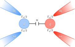
Figure 1: (Color online) Illustration of the model system studied: two quantum impurities, $d$ and $q$, capacitively coupled with interaction strength $u$. Each impurity $i(=d,\,q)$ is coupled to its own set of metallic terminals with hybridization energy $\Gamma_{i}/2$.

The Kondo effectKondo (1964); Ng and Lee (1988); Glazman and Raǐkh (1988); Pustilnik and Glazman (2001) is a paradigmatic many–body phenomenon that has been repeatedly observed in QDs since the late 1990s,Goldhaber-Gordon et al. (1998) and whose understanding is of fundamental importance in condensed matter physics.Hewson (1993) It arises due to spin or pseudospinBorda et al. (2003); Hübel et al. (2008); Okazaki et al. (2011) correlations between a quantum impurity and the itinerant electrons in the metallic reservoir in which it is embedded. The important role of the Kondo effect in the behavior of complex nanoscale systems has been demonstrated time and again: It has been observed in measurements of the dephasing by a quantum point contact (a charge detector on a nearby QD),Avinun-Kalish et al. (2004) while an unusual variety of Kondo effect with SU(4) symmetry was theoretically predictedGalpin et al. (2005a, b) and recently observed experimentallyAmasha et al. (2013); Keller et al. (2014) in a system of two identical, capacitively coupled QDs. Many other examples exist.van der Wiel et al. (2002) Capacitively coupled QDs have been recently predicted to exhibit a spatial rearrangement of the screening cloud under the influence of a magnetic field.Vernek et al. (2014)

In this work we present a study of the correlated transport regimes of a system of two independently contacted quantum impurities, each possibly in the Kondo regime, and coupled to each other through capacitive interactions (see Fig. 1). We aim to understand how the Kondo correlations in one of them are affected by the presence and controlled variation of the other subsystem. To this end, we carry out an analysis of the coupled system within the Kondo regime. The study utilizes a variational, as well as a numerical approach to the problem. The variational analysis gives us interesting insights into the effects of the capacitive coupling on the ground state of the coupled QD system. We further evaluate dynamic and thermodynamic properties of the system using the numerical renormalization group (NRG) method. We put especial emphasis on the conductances of both subsystems, which can be measured experimentally.

Our results show that the effects of the capacitive coupling can be absorbed into a positive shift of the local energies of the impurities, as one could anticipate. However, for the generic case of non–identical subsystems, the size of the effective shifts strongly depend on the relative magnitudes of the level depths with respect to the Fermi level, and the hybridization of each impurity to its electronic reservoirs. Moreover, the asymmetric shifts for effectively large capacitive coupling can drive the ‘shallower’ subsystem into a mixed–valence regime, or even further away from the Kondo regime, resulting in interesting behavior of the relative Kondo temperature(s) and response functions, including the conductance levels through the separately–connected subsystems. Interestingly, a suppression of the unitary conductance produced by the Kondo effect is observed in the shallow impurity when the level shift produces a quantum phase transition out of the Kondo regime. These changes illustrate an interesting modulation of the Kondo correlations in one subsystem by a purely capacitive coupling, which could perhaps be useful in more general geometries.

In fact, all of the regimes presented in this paper are already accessible to experiments with double quantum dots, and may be of relevance for other types of quantum impurity systems as well. One can think in particular of the often used configuration, where a charge detector [a properly biased quantum point contact (QPC)] is placed in close proximity to an active QD. It is known that a QPC exhibits Kondo correlations,Rejec and Meir (2006) which will be clearly affected by the capacitive coupling to the dot. With this in mind, in what follows we refer to the two independently connected impurities as the QD ($d$) and the QPC detector ($q$), and consider regimes where they can be seen as spin–$\frac{1}{2}$ quantum impurities coupled to their corresponding set of current leads.

II Model

We model the two subsystems as single–level Anderson Hamiltonians of the form

$$\begin{split}H_{d}=&\varepsilon_{d}\,n_{d}+U_{d}\,n_{d\uparrow}n_{d\downarrow}+\sum_{\mathbf{k}\sigma}\varepsilon_{k\sigma}n_{d\mathbf{k}\sigma}\\ &+V_{d}\sum_{\mathbf{k}\sigma}\left(d_{\sigma}^{\dagger}c_{d\mathbf{k}\sigma}+\text{H. c.}\right),\end{split}$$ (1a)

$$\begin{split}H_{q}=&\varepsilon_{q}\,n_{q}+U_{q}\,n_{q\uparrow}n_{q\downarrow}+\sum_{\mathbf{k}\sigma}\varepsilon_{k\sigma}n_{q\mathbf{k}\sigma}\\ &+V_{q}\sum_{\mathbf{k}\sigma}\left(q_{\sigma}^{\dagger}c_{q\mathbf{k}\sigma}+\text{H. c.}\right),\end{split}$$ (1b)

where the subindices $d$ and $q$ indicate the QD and the QPC, respectively, and $\varepsilon_{d}$ and $\varepsilon_{q}$ are the energies of the corresponding local levels; the number operators are given by $n_{i}=\sum_{\sigma}n_{i\sigma}$, with $\sigma=\uparrow,\,\downarrow$, and $U_{i}$ is the energy cost of double occupancy of level $i=d,\,q$ due to intra–impurity Coulomb interactions. The number operators $n_{i\mathbf{k}\sigma}$ give the occupation of the state of momentum $\mathbf{k}$ and spin projection $\sigma$ of the metallic terminal coupled to dot $i$. We consider here a band of half–bandwidth $D$ for each lead, with a flat density of states $\rho(\varepsilon)=\Theta(D-|\varepsilon|)/2D$, where $\Theta(x)$ is the Heaviside function. Assuming that the two terminals attached to each impurity are identical, we define the symmetric operators $c_{i\mathbf{k}\sigma}=\left(c_{iL\mathbf{k}\sigma}+c_{iR\mathbf{k}\sigma}\right)/\sqrt{2}$— with indices $L$ and $R$ for the left and right terminals, respectively— to which the impurity couples exclusively. The full Hamiltonian is thus

$$H=H_{d}+H_{q}+u\,n_{d}n_{q},$$ (2)

where the mutual capacitive coupling is parameterized by the energy $u>0$. The extra energy cost of simultaneous occupation of both impurities will produce a competition between their otherwise separate ground states: In the case of $\varepsilon_{i}<0$ and $\Gamma_{i}=\pi|V_{i}|^{2}/(2D)\ll\left|\varepsilon_{i}\right|$, for both $i=d,\,q$, it would be favorable for each impurity to be singly occupied. The capacitive coupling, however, raises the energy of this coupled configuration and, depending on the magnitude of $u$, another occupancy may be more energetically favorable.

For interacting quantum impurities ($U_{i}>0$) within this parameter regime, the Kondo effectKondo (1964); Goldhaber-Gordon et al. (1998) takes place for temperatures below a characteristic temperature scale $T_{K}^{i}$. However, as we find below, the added energy cost of having a charge in a given impurity may drive the other impurity out of the Kondo regime at a critical coupling, as the mixed–valence regime is reached.

In order to understand the competition between different impurities’ ground states, we use the variational approach described in Appendix A. Because there is no charge exchange between the two subsystems, the effect of the capacitive coupling on each impurity can be absorbed into a level shift of the form $\varepsilon_{i}\rightarrow\varepsilon_{i}+\Lambda_{i}$, with each $\Lambda_{i}>0$ depending on the parameters of both quantum impurities, and on $u$. This shift can then be extracted variationally from a proposed wave function based on the form expected in the strong-coupling fixed point (SCFP) of the uncoupled systems,Krishna-murthy et al. (1980a, b) where the ground state has a many–body singlet structure. The level shifts $\Lambda_{d}$ and $\Lambda_{q}$ can be calculated by minimizing the energy of the coupled system. Within each subsystem, the corresponding level shift $\Lambda_{i}$ can be interpreted as an external gate voltage that raises the dot level, and thus determines the nature of its ground state.Ferreira et al. (2011)

In what follows, we describe the results of both the variational and NRG approaches, and explore the resulting physics and measurable consequences of the capacitive coupling. The NRG calculations fully capture the many–body correlations of the problem, and allow us to reliably calculate expectation values of operators, as well as the dynamic and thermodynamic properties of the system.

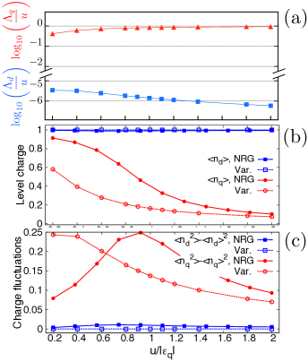
Figure 2: (Color online) (a) External gating of the impurity levels, $\Lambda_{d}$ and $\Lambda_{q}$ for identical couplings ($\Gamma_{d}=\Gamma_{q}=0.002\,D$), but asymmetric impurities, with $\varepsilon_{d}=-0.025\,D$, $\varepsilon_{q}=-0.010\,D$ and varying $u$, as obtained variationally. (b) Charge and (c) charge fluctuations of both impurities evaluated using the variational method and NRG, showing how impurity $q$ is depleted as the capacitive coupling $u$ is increased, while impurity $d$ remains essentially unchanged. The NRG calculations were carried out with local Coulomb interaction strengths of $U_{d}=U_{q}=0.05\,D$.

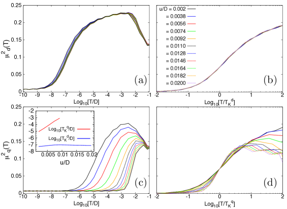
Figure 3: (Color online) Magnetic–moment–squared of impurities (a) $d$ and (c) $q$ as functions of the temperature, for different values of the capacitive coupling $u$, as shown in the legend in panel (b); all panels show results for the same set of $u$ values. (b) and (c) show the same quantities as functions of temperature, normalized to the Kondo temperature of each curve. The inset of (c) shows the dependence of the Kondo temperatures on $u$. All results obtained from NRG calculations. Parameters correspond to those of Fig. 2. Notice that for $u\gtrsim 0.01\,D$ impurity $q$ is pushed away from the Kondo regime, first into mixed–valence, eventually reducing $n_{q}$ well below unity (see Fig. 2).

III Effective gating due to capacitive coupling

Results from the variational method are shown in Figure 2(a) as function of the capacitive coupling $u$, for impurities with identical couplings to their respective metallic leads. While $\varepsilon_{d}\ll-\Gamma_{d}$ is fixed deep in the Kondo regime, and $\varepsilon_{q}(\geq\varepsilon_{d})$ is set closer to the mixed valence regime ($\varepsilon_{q}\lesssim-\Gamma_{q}$), we see that increasing $u$ affects both subsystems asymmetrically. As $u$ increases, the level of impurity $q$ is raised ($\Lambda_{q}$ increases), while the remote gate effect due to the capacitive coupling vanishes for impurity $d$ ($\Lambda_{d}$ decreases). The remote gate then becomes effectively larger for impurity $q$, indicating that the “shallower” level is more susceptible to the capacitive coupling. One can qualitatively understand this behavior by examining how a shift in $\varepsilon_{q}$ affects the Kondo temperature. Substituting $\varepsilon_{q}\rightarrow\varepsilon_{q}+\Lambda_{q}$ into the expression for the Kondo temperature within the variational frameworkVarma and Yafet (1976)

$$T_{K}^{i}=D\exp\left(-\pi\left|\varepsilon_{i}\right|/\Gamma_{i}\right),$$ (3)

and evaluating its total differential as a function of $\Lambda_{q}$, we find

$$\mathrm{d}T_{K}^{q}\equiv\frac{\partial T_{K}^{q}}{\partial\varepsilon_{q}}\mathrm{d}\varepsilon_{q}=-\Lambda_{q}\,\frac{\text{sgn}\left[\varepsilon_{q}\right]\,\pi D}{\Gamma_{q}}\,\exp(-\pi|\varepsilon_{q}|/\Gamma_{q}),$$ (4)

which is proportional to $\Lambda_{q}$ and grows exponentially as $\left|\varepsilon_{q}\right|$ becomes smaller. Notice that the Kondo temperature is a measure of how much the impurity hybridization contributes to the lowering of the ground state energy of each subsystem due to the onset of many-body correlations, with respect to the atomic limit ($\Gamma_{q}=0$). The essence of Eq. (4) is that it is energetically favorable for the “shallower” level to be shifted the most when the coupling increases. A maximum shift of $\Lambda_{q}\approx u$ for large values of $u$ is in accordance with Eqs. (19a) and (19b).

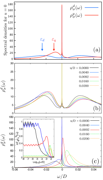
Figure 4: (Color online) Spectral densities of both impurities for varying capacitive coupling $u$, for parameters $U_{d}=U_{q}=0.05\,D$, $\varepsilon_{d}=-U_{d}/2=-0.025\,D$, $\varepsilon_{q}=-0.010\,D$ and $\Gamma_{d}=\Gamma_{q}=0.002\,D$. (a) Reference curves with $u/D=0$, showing the local levels dressed by their respective electronic reservoirs, and the ASR of each impurity at the Fermi level. Same $u=0$ curves shown in black in corresponding (b) and (c) panels. (b) The ASR of impurity $d$ remains well–defined for all values of $u$. The panel focuses on the Hubbard bands, amplifying the lower region of the vertical axis for clarity (notice different scale). (c) In the case of impurity $q$, the disappearance of the ASR and the shift of the left Hubbard peak toward positive values of $\omega$ with increasing $u$ is a clear indication that the Kondo effect is being quenched. Inset in (c) shows detailed behavior of $\rho_{\sigma}^{q}(\omega)$ for $\omega\approx 0$. For $u\gtrsim 0.01\,D$, the $q$-impurity is pushed out of the Kondo regime.

A comparison between the variational and NRG approaches is shown in Fig. 2(b), where the charges and charge fluctuations of both impurities are presented. Impurity $q$ is depleted due to the external gating produced by the capacitive coupling, in both calculations. Although it is clear from comparing to the NRG results that the variational method overestimates the strength of the gating—likely a consequence of the infinite-$U_{i}$ approximation that allows the simple form of the proposed ground state—the behavior predicted by both methods is qualitatively consistent. As $u$ increases, $\langle n_{q}\rangle$ decreases to zero, while $\langle n_{d}\rangle$ remains essentially constant $\simeq 1$. Correspondingly, the characteristic fluctuations in $q$ are significant and peak (at $\langle n_{q}\rangle\simeq\frac{1}{2}$), whereas those in $d$ remain small throughout.

Turning to the thermodynamic properties of the system, Figs. 3(a) and (c) show the temperature dependence of the effective magnetic–moment–squared of impurities $d$ and $q$, respectively, given by $\mu_{i}(T)=T\,\chi_{i}(T)$, with $\chi_{i}$ the magnetic susceptibility of impurity $i$. Different curves correspond to different values of the capacitive coupling. The Kondo temperature in each case can be obtained from each curve [$T_{K}^{i}\chi(T_{K}^{i})=0.0707$], and the temperature axis can be rescaled as in Figures 3(b) and (d), in order to collapse all curves into the universal curve that is the hallmark of Kondo physics.Wilson (1975) All curves for the $d$-impurity demonstrate this universal behavior in Fig. 3(b). Notice, however, that impurity–$q$ curves for $u/D>0.0092$ fall outside the universality curve in Fig. 3(d), indicating a transition away from the Kondo regime for large $u$, which from the variational analysis can be understood as the large gating coming from the capacitive coupling. This is consistent with the depletion of impurity $q$ shown in Fig. 2(b). The exponential dependence of the Kondo temperature $T_{K}^{q}$ on $u$ [see Eq. (3)], shown in the inset of Fig. 3(c), is further confirmation of this picture. It is important to emphasize that increasing the gating on impurity $q$ at first enhances its Kondo temperature. However, beyond a critical value of $u$, the impurity reaches the mixed–valence regime, and is eventually emptied out. In contrast, as the shallower impurity is depleted by the gating, the Kondo temperature $T_{K}^{d}$ of impurity $d$ is in fact restored to its uncoupled value, as the inset of Fig. 3(c) shows.

To complete our analysis of this case, we present the local spectral density of the impurities in Fig. 4. The spectral density of impurity $q$ is defined as

$$\rho_{\sigma}^{q}(\omega)=-\frac{1}{\pi}\text{Im}\langle\langle q_{\sigma};\,q_{\sigma}^{\dagger}\rangle\rangle_{\omega},$$ (5)

with $\langle\langle A;\,B\rangle\rangle_{\omega}$ the retarded Green’s functionZubarev (1960) of operators $A$ and $B$. It represents the effective single–particle level density available at energy $\omega$, at the impurity site: the left peak at $\omega/D\approx-0.01$ of the curve for $u/D=0$ in Fig. 4(a) (solid red line) corresponds to the occupied impurity level, dressed by the leads’ electrons. The sharp peak at $\omega/D=0$ is the Abrikosov–Suhl resonance (ASR)— a typical signature of the Kondo effect.Abrikosov (1965); Suhl (1965); Nagaoka (1965) As the capacitive coupling increases, there is a clear progression of the effective $q$-level toward positive values, as seen in Fig. 4(c), eventually quenching the Kondo effect at $u/D\approx 0.0092\,D$, when the charge fluctuations peak, and the charge is reduced by 50% (see Fig. 2). In fact, assuming a simple linear shift of $\varepsilon_{q}\rightarrow\varepsilon_{q}+u$ would suggest that the mixed–valence regime will be reached for $u\approx|\varepsilon_{q}|-\Gamma_{q}$, in agreement with the variational result [Fig. 2(a)] that yields $\Lambda_{q}\rightarrow u$ for $u\rightarrow|\varepsilon_{q}|$. That the Kondo effect is quenched for slightly larger $u$ reflects the overestimation of the remote gating by the variational method, as mentioned above. Figure 4(c) also shows that for $u\gtrsim 0.0092\,D$, the ASR at the Fermi level disappears in the spectral function for the $q$-impurity, and the (now emptying) single–particle resonance moves increasingly above the Fermi level. The inset in Fig. 4(c) examines the behavior of the $\rho^{q}_{\sigma}$ near the Fermi level, showing again its decreasing value, vanishing for $u\gtrsim 0.0092\,D$ as well. The spectral density $\rho_{\sigma}^{d}(\omega)$, on the other hand, shows only a slight, non–monotonic shift of the impurity–$d$ level, with a stable ASR for all values of the capacitive coupling, also in agreement with the variational result [see Fig. 4(b)].

IV The role of particle–hole symmetry in the coupled system

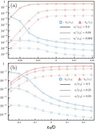
Figure 5: (Color online) External gating of the impurity levels, $\Lambda_{d}$ and $\Lambda_{q}$ as a function of $\varepsilon_{q}$, as obtained from the variational calculation. (a) For impurities with identical couplings ($\Gamma_{d}=\Gamma_{q}=0.002\,D$), with fixed $\varepsilon_{d}=-0.025\,D$. (b) For different couplings ($\Gamma_{d}=0.002\,D$, $\Gamma_{q}=0.05\,D$), with fixed $\varepsilon_{d}=-0.02\,D$.

Armed now with the basic understanding of the inter–impurity coupling model, we turn to a setup that is commonly implemented in experiments. It is possible to independently tune the impurity levels in a QD sample by means of gate voltages—a common practice in electron counters for QDsGustavsson et al. (2006) and “which path” interferometers.Aleiner et al. (1997); Buks et al. (1998); Avinun-Kalish et al. (2004) We study now the coupled system when one of the quantum impurity levels is controlled by an external gate.

Considering again the case $\Gamma_{d}=\Gamma_{q}$, Fig. 5(a) shows results of the variational method for different fixed values of $u$, while varying $\varepsilon_{q}$ but keeping $\varepsilon_{d}=-0.025\,D$ fixed. Starting at $\varepsilon_{q}=\varepsilon_{d}$, both impurities experience the same gating $\Lambda_{d}=\Lambda_{q}$, as one would expect from symmetry arguments. As the level of impurity $q$ moves closer to the Fermi energy, $\Lambda_{q}$ grows quickly, while $\Lambda_{d}$ decreases. Once again, it is clear that the shallower level— that of impurity $q$— experiences a larger gating. Notice that the asymmetry persists even for small $u$, where $\Lambda_{q}$ grows fast, while $\Lambda_{d}$ drops only slightly. This general behavior of the $\Lambda_{i}$ persists for impurities with different lead couplings, as can be seen in Fig. 5(b), which shows results for $\Gamma_{q}=0.05\,D$, $\Gamma_{d}=0.002\,D$ and $\varepsilon_{d}=-0.02\,D$. The asymmetry of the subsystems is reflected in the different values of $\Lambda_{d}$ and $\Lambda_{q}$, even for $\varepsilon_{q}\leq\varepsilon_{d}$.

Naturally, in a QD system one can monitor the different ground states via conductance measurements. In Fig. 6 we present NRG calculations of the zero–bias conductance through each impurity, with $\varepsilon_{d}$ fixed while $\varepsilon_{q}$ is varied. The conductance profile of impurity $q$ remains approximately the same for all three values of $\varepsilon_{d}$ shown; it is, in fact, nearly identical to the case of a completely independent impurity ($u=0$), since it is so deep into the Kondo regime and the interaction $u$ does not affect it much. Impurity $d$— here the shallower one—, on the other hand, is strongly affected by the capacitive coupling, especially for $\varepsilon_{q}<-U_{q}/2$, when $\left<n_{q}\right>>1$ (Fig. 6). While its bare parameters are within the Kondo regime, the enhanced conductance of impurity $d$— characteristic of the Kondo effect— is strongly suppressed as the capacitive coupling to $q$ shifts $\varepsilon_{d}$ effectively, and reduces its average charge [Fig. 6(c)]. In accordance with the Friedel sum rule,Hewson (1993) the conductance per spin channel at zero temperature is given by

$$G_{d\sigma}(T=0)=\frac{e^{2}}{h}\,\sin\left(\pi\left<n_{d\sigma}\right>\right),$$ (6)

and so it will be reduced as $\left<n_{d\sigma}\right><1$. The conductance curves in Fig. 6(b) reflect the variation of $\left<n_{d\sigma}\right>$ as the gate applied to impurity $q$ shifts its level [Fig. 6(b)], and it shows how the enhanced conductance may be reduced as a consequence of the equilibrium charge fluctuations in the impurity. This effect is naturally more pronounced for $\varepsilon_{d}$ closer to the Fermi level, yet well into the Kondo regime for $u=0$.

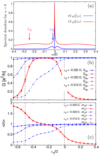
Figure 6: (Color online) (a) Comparison of the spectral densities of both impurities (in the electron–hole symmetric regime, $\varepsilon_{d}=-U_{d}/2$), when $\Gamma_{q}\gg\Gamma_{d}$ and $U_{q}\gg U_{d}$. (b) Conductances per spin channel (in units of $e^{2}/h$) for impurities $d$ and $q$, and (c) their occupations, as functions of $\varepsilon_{q}$, for different values of $\varepsilon_{d}$. All results from NRG calculations; parameters: $U_{d}=0.05\,D$, $U_{q}=0.5\,D$, $\Gamma_{d}=0.002\,D$, $\Gamma_{q}=0.05\,D$, $u=0.01\,D$. Vertical dashed lines denote the region in the uncoupled regime ($u=0$) for impurity $q$ ($\langle n_{q}\rangle=1$) where the high conductance in the Kondo regime is expected.

The influence of the remote gating from impurity $q$ on impurity $d$ is perhaps more clearly appreciated in Fig. 7, which shows the Kondo temperatures of both impurities as functions of $\varepsilon_{q}$. The termination of each of the curves indicate the (approximate) values of $\varepsilon_{q}$ at which the Kondo effect is quenched in either impurity. As in the conductance results, the curves for impurity $q$ are nearly identical to the independent impurity limit. The curves of $T_{K}^{d}$, on the other hand, show a plateau structure that directly relates to $\left<n_{q\sigma}\right>$ [see Fig. 6(c)]: As $\varepsilon_{q}$ grows more negative, the remote gating on $d$ increases with $u\left<n_{q}\right>$—the energy contribution of the capacitive coupling—raising the level of impurity $d$, and consequently increasing $T_{K}^{d}$ until the Kondo effect is quenched. This transition is indicated by the black, dashed trend line in the figure. As the remote gating decreases (with increasing $\varepsilon_{q}$) and the enhanced conductance is restored in $d$, the Kondo temperature $T_{K}^{d}$ is reduced back to its value in the electron–hole symmetric case. At this point, it is impurity $q$ that is gated the most, but given that $|\varepsilon_{q}|\gg u$, the effects of this gating are not noticeable in either the conductance or the Kondo temperatures. Notice that, as the $q$-impurity is emptied ($\varepsilon_{q}>0$), $T_{K}^{d}$ settles into the isolated $d$-impurity value.

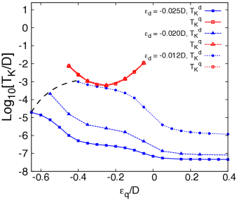
Figure 7: (Color online) Kondo temperatures $T_{K}^{d}$ and $T_{K}^{q}$ of impurities $d$ and $q$, respectively, as functions of $\varepsilon_{q}$, for three fixed values of $\varepsilon_{d}$. The curves terminate, indicating the approximate values of $\varepsilon_{q}$ at which the Kondo effect is quenched in each case. The dashed line on the left indicates the trend of the transition out of the Kondo regime for impurity $d$. All other parameters as in Fig. 6.

The same conductance analysis is repeated in Fig. 8, this time varying the level of impurity $d$, which has the smaller parameters $U_{d}$ and $\Gamma_{d}$. The gating effects on impurity $q$ are negligible, with only a slight drop in conductance (about $10\%$) in the case of $\varepsilon_{q}=-0.010\,D$, when it is on the edge between the Kondo phase and the mixed–valence regime. Most noticeable is the overall shift of $\approx u$ on the conductance profile of impurity $d$ to lower $\varepsilon_{d}$ values, as a result of the gating.

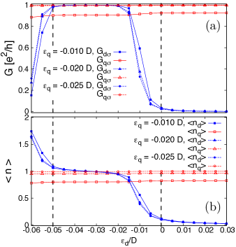
Figure 8: (Color online) NRG calculations of (a) the conductance of impurities $d$ and $q$, and (b) the occupation of both impurities, as functions of $\varepsilon_{d}$, for different values of $\varepsilon_{q}$. Parameters: $U_{d}=0.05\,D$, $U_{q}=0.5\,D$, $\Gamma_{d}=0.002\,D$, $\Gamma_{q}=0.05\,D$, $u=0.01\,D$. Vertical dashed lines indicate the region $\langle n_{d}\rangle=1$ for the uncoupled case ($u=0$). Notice the typical conductance plateau is shifted by $\approx u$ to lower $\varepsilon_{d}$ values due to the remote gating effect.

The results presented in this section are summarized in Fig. 9, which shows the phase diagrams for both subsystems. Figure 9(a) shows the quenching of the Kondo effect in impurity $q$ by the capacitive coupling strength $u$ for fixed $\varepsilon_{d}$, as a transition from $\left<n_{q}\right>=1$ to $0$, for any given value of $\varepsilon_{q}$ within the colored region. Fig. 9(b) demonstrates how the $d$-impurity undergoes this transition only for $\varepsilon_{q}<\varepsilon_{d}$, when it becomes the shallower level. The two slopes of the left boundary of the colored region indicate different behaviors of impurity $d$ when $\left<n_{q}\right>=1$ and $2$. The location of these boundaries are inferred from the behavior of the Kondo temperatures as the structure parameters change. $T_{K}^{d}$ and $T_{K}^{q}$ are shown in the middle panel of the figure for typical cases. In the upper panel, $q$ is the shallower subsystem ($|\varepsilon_{q}|/\Gamma_{q}\ll|\varepsilon_{d}|/\Gamma_{d}$), and as $u$ increases it is $q$ which is effectively gated into the empty impurity regime. The middle panel shows a fully symmetric case, where large $u$ destroys the Kondo regime in both subsystems simultaneously. Finally, the bottom panel shows the case where $d$ is shallower ($|\varepsilon_{q}|/\Gamma_{q}\gg|\varepsilon_{d}|/\Gamma_{d}$) such that the gating destroys the Kondo correlations in $d$. In the asymmetric cases, it is also clear that as the other subsystem is gated into the empty regime, the Kondo temperature of the remaining impurity reverts to the isolated value for increasing $u$.

Figures 9(c) and (d) illustrate the phase diagram for fixed $u$, while varying $\varepsilon_{d}$ and $\varepsilon_{q}$. Because $|\varepsilon_{q}|$ is very large with respect to $u$, the transition out of Kondo is induced only on impurity $d$, whose level depth $\varepsilon_{d}$ is comparable to the capacitive coupling strength $u$. This transition, induced by the presence of impurity $q$, is shown as the left boundary to the blue region in panel (c), and occurs for lower values of $\varepsilon_{d}$ as $\left<n_{q}\right>$ grows (for more negative values of $\varepsilon_{q}$) and the capacitive interaction strength increases.

These results are important and should be considered in the analysis of coupled systems, such as the decoherence studies where the suppression of the zero–bias conductance through the QD is used to measure the dephasing rate of a nearby charge detector.Avinun-Kalish et al. (2004) As shown in Fig. 6, the capacitive coupling between the two impurities in equilibrium can significantly suppress the enhanced conductance expected of the quantum dot, by virtue of the competition it introduces between the impurities’ ground states. Charge detectors for quantum dots are commonly implemented using a quantum point contact, and it has been suggestedAono (2008) that the anomalous behavior observed in the dephasing rate of the QPC in the experiments of Ref. [Avinun-Kalish et al., 2004] is due to the appearance of a localized level within the QPC, which can undergo Kondo screening.Meir et al. (2002) Our study is thus highly relevant for the interpretation and full analysis of these and similar experiments, as it presents an equilibrium analysis of the experimental setup, which is typically treated as a static system (the limit of Fig. 8). We demonstrate that, in some parameter regimes, the ground state of the system is in fact quite sensitive to capacitive coupling, and the equilibrium charge fluctuations of one of the impurity subsystems are able to strongly influence the conductance of the other. This sensitivity makes it a much more subtle task to evaluate how much of the conductance suppression in one subsystem is due to the dephasing induced by the other.

V Conclusions

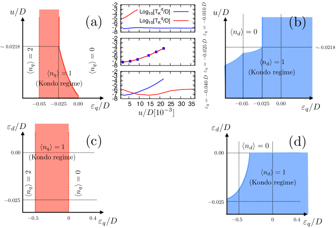
Figure 9: (Color online) Schematic $u$-$\varepsilon_{q}$ phase diagrams for (a) impurity $q$ and (b) impurity $d$, for fixed $\varepsilon_{d}=-0.025\,D$, with $U_{d}=U_{q}=0.05\,D$ and $\Gamma_{d}=\Gamma_{q}=0.002\,D$. The Kondo temperatures of both impurities for select values of $\varepsilon_{q}$ are shown in the central panels, as functions of $u$. (c) and (d) show the phase diagrams in the $\varepsilon_{d}$-$\varepsilon_{q}$ plane for impurities $q$ and $d$, respectively, for fixed $u=0.01\,D$, with $U_{d}=0.05\,D$, $U_{q}=0.5\,D$, $\Gamma_{d}=0.002\,D$ and $\Gamma_{q}=0.05\,D$. The shaded areas indicate that the corresponding impurity is in the Kondo regime. The Kondo temperatures are higher closer to the boundaries of the shaded regions.

We have studied the Kondo physics of a system of two capacitively–coupled quantum impurities, by means of both a variational method and numerical renormalization group calculations. We found that the capacitive interaction can be absorbed into an external gating effect that varies non–linearly with the capacitive coupling strength, as well as the impurities’ energy levels. We demonstrate that the external gating to one impurity coming from the other can induce a quantum phase transition out of the Kondo regime, modifying its conductance properties in a way that can be measured experimentally. Our results suggest that, as the subtle balance of interactions strongly affects the nature of this type of system in certain parameter regimes, it is of great relevance to the study of dephasing effects of charge detectors on quantum dots, where conductance suppression is used as a measure of the dephasing rate.

Appendix A Variational calculation of the two–impurity Kondo ground state

We use a variational approach following the methods of Ref. [Varma and Yafet, 1976], where a variational wavefunction for the ground state is proposed based on the many–body singlet nature of the Kondo state. The $d$-impurity ground state is given by

$$\left|\psi_{d}\right>=\left[\beta_{0}+\sum_{\mathbf{k}\sigma}d_{\sigma}^{\dagger}\beta_{\mathbf{k}}\,c_{d\mathbf{k}\sigma}\right]\left|\Omega_{d}\right>,$$ (7)

with the state

$$\left|\Omega_{d}\right>=\prod_{\left|\mathbf{k}\right|<k_{F}}{c_{d\mathbf{k}\uparrow}}^{\dagger}{c_{d\mathbf{k}\downarrow}}^{\dagger}\left|0\right>,$$ (8)

representing the leads filled up to the Fermi momentum $k_{F}$. The corresponding state for impurity $q$ is

$$\left|\psi_{q}\right>=\left[\alpha_{0}+\sum_{\mathbf{k}\sigma}q_{\sigma}^{\dagger}\alpha_{\mathbf{k}}\,c_{q\mathbf{k}\sigma}\right]\left|\Omega_{q}\right>.$$ (9)

The set of (real) coefficients $\alpha=\{\alpha_{0},\,\alpha_{\mathbf{k}}\}$ and $\beta=\{\beta_{0},\,\beta_{\mathbf{k}}\}$ are variational parameters. These variational states are expected to be more reliable in the limit of large $U_{i}$, as double occupancy is omitted. The full state of the coupled system is then proposed as

$$\left|\Psi_{\text{gnd}}\right>=\left|\psi_{q}\right>\otimes\left|\psi_{d}\right>,$$ (10)

and the energy contribution from the impurities is given by

$$E(\alpha,\,\beta)=\frac{\big{<}\Psi_{\text{gnd}}\big{|}H\big{|}\Psi_{\text{gnd}}\big{>}}{\left<\Psi_{\text{gnd}}\right|\left.\Psi_{\text{gnd}}\right>}=E_{d}+E_{q}+\tilde{u},$$ (11)

where we have defined the separate impurity energy contributions

$$E_{q}=2\left<\psi_{q}\right>^{-1}\sum_{\left|\mathbf{k}\right|<k_{F}}\left[\left(\varepsilon_{q}-\varepsilon_{\mathbf{k}}^{q}\right)\alpha_{\mathbf{k}}^{2}-2V_{q}\alpha_{0}\alpha_{\mathbf{k}}\right],$$ (12)

$$E_{d}=2\left<\psi_{d}\right>^{-1}\sum_{\left|\mathbf{k}\right|<k_{F}}\left[\left(\varepsilon_{d}-\varepsilon_{\mathbf{k}}^{d}\right)\beta_{k}^{2}-2V_{d}\beta_{0}\beta_{\mathbf{k}}\right],$$ (13)

and the capacitive coupling contribution

$$\tilde{u}=u\,\frac{\left(2\sum_{\left|\mathbf{k}\right|<k_{F}}\alpha_{\mathbf{k}}^{2}\right)\left(2\sum_{\left|\mathbf{k}\right|<k_{F}}\beta_{\mathbf{k}}^{2}\right)}{\left<\psi_{d}\right|\left.\psi_{d}\right>\left<\psi_{q}\right|\left.\psi_{q}\right>}.$$ (14)

We then proceed to minimize the ground state energy Eq. (11) with respect to the variational amplitudes by the conditions

$$\frac{\partial}{\partial\alpha_{0}}E(\alpha,\,\beta)=\frac{\partial}{\partial\alpha_{k}}E(\alpha,\,\beta)=0,$$ (15a)

$$\frac{\partial}{\partial\beta_{0}}E(\alpha,\,\beta)=\frac{\partial}{\partial\beta_{k}}E(\alpha,\,\beta)=0.$$ (15b)

The resulting variational equations are

$$2V_{q}\sum_{\left|\mathbf{k}\right|<k_{F}}\alpha_{\mathbf{k}}=\alpha_{0}\left(E_{q}+\tilde{u}\right),$$ (16a)

$$\begin{split}\alpha_{0}V_{q}=\alpha_{\mathbf{k}}\Big{[}&E_{q}-\left(\varepsilon_{q}-\varepsilon_{\mathbf{k}}^{q}\right)\\ &-2u\,\alpha_{0}^{2}\left<\Psi_{\text{gnd}}\right|\left.\Psi_{\text{gnd}}\right>^{-1}\sum_{\left|\mathbf{k}\right|<k_{F}}\beta_{\mathbf{k}}^{2}\Big{]},\end{split}$$ (16b)

and a completely identical set for $d$ (i.e., $q\rightarrow d$ and $\alpha\rightarrow\beta$). We propose the relations $\alpha_{\mathbf{k}}\equiv\alpha_{k}$ and $\beta_{\mathbf{k}}\equiv\beta_{k}$, with

$$\alpha_{k}=\frac{\alpha_{0}V_{q}}{\varepsilon_{k}^{q}-\varepsilon_{q}-\Lambda_{q}+E_{q}},$$ (17a)

$$\beta_{k}=\frac{\beta_{0}V_{d}}{\varepsilon_{k}^{d}-\varepsilon_{d}-\Lambda_{d}+E_{d}},$$ (17b)

and substitute into Eqs. (16) and the corresponding equations for impurity $d$ to obtain (in the continuum limit)

$$\begin{split}\frac{V_{d}^{2}}{D}\log\left[\frac{\varepsilon_{q}-E_{d}-\varepsilon_{F}+\Lambda_{q}}{\varepsilon_{q}-E_{q}+D+\Lambda_{q}}\right]=&\\ E_{q}+u\frac{X_{q}X_{d}}{\left(1+X_{q}\right)\left(1+X_{d}\right)},&\end{split}$$ (18a)

$$\begin{split}\frac{V_{q}^{2}}{D}\log\left[\frac{\varepsilon_{d}-E_{q}-\varepsilon_{F}+\Lambda_{d}}{\varepsilon_{d}-E_{d}+D+\Lambda_{d}}\right]=&\\ E_{d}+u\frac{X_{q}X_{d}}{\left(1+X_{q}\right)\left(1+X_{d}\right)},&\end{split}$$ (18b)

$$\Lambda_{d}=u\frac{X_{q}}{\big{(}1+X_{d}\big{)}\big{(}1+X_{q}\big{)}},$$ (19a)

$$\Lambda_{q}=u\frac{X_{d}}{\big{(}1+X_{d}\big{)}\big{(}1+X_{q}\big{)}}.$$ (19b)

where we have defined the continuum–limit quantities

$$\alpha_{0}X_{q}=2\sum_{k<k_{F}}\alpha_{k}^{2}\rightarrow\frac{V_{q}^{2}}{\left(\varepsilon_{q}-E_{q}+\Lambda_{q}\right)\left(\varepsilon_{q}-E_{q}+D+\Lambda_{q}\right)},$$ (20a)

$$\beta_{0}X_{d}=2\sum_{k<k_{F}}\beta_{k}^{2}\rightarrow\frac{V_{d}^{2}}{\left(\varepsilon_{d}-E_{d}+\Lambda_{d}\right)\left(\varepsilon_{d}-E_{d}+D+\Lambda_{d}\right)}.$$ (20b)

This system of equations is then solved numerically, in terms of $\Lambda_{d}$ and $\Lambda_{q}$. From these solutions, and using Eqs. (20a) and (20b), we directly obtain the charge and charge fluctuations of each impurity.

Appendix B The conductance profile of an interacting quantum impurity

As a reference to the results shown in Figs. 6 through 8, in this section we show the typical zero–temperature behavior of the zero–bias conductance of a single interacting spin–1/2 quantum impurity, hybridizing with metallic leads. Parameters are $U_{q}=0.5\,D$, $\Gamma_{q}=0.05\,D$, with $D$ (the half–bandwidth of the leads’ density of states) being used as an energy unit.

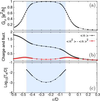
Figure 10: (Color online) Typical (a) conductance (per spin channel) and (b) charge and charge fluctuation profiles (full and empty circles, respectively) of an interacting quantum impurity, as functions of the level energy $\varepsilon$. (c) Kondo temperature as a function of $\varepsilon$. The shaded region represents the range of $\varepsilon/D$ where the Kondo effect takes place. Curves calculated using NRG. Parameters: $U_{q}=0.5\,D$, $\Gamma_{q}=0.05\,D$.

Figure 10(a) shows the variation of the conductance through the impurity: Coherent transport through the impurity is possible only when the impurity level is resonance with leads’ Fermi level ($\varepsilon_{F}=0$). The conductance is thus zero for $\varepsilon_{q}>0$. Lowering the impurity level below zero, and within a range $\Gamma_{q}$ of the Fermi level, the conductance begins to rise as the system enters the mixed–valence regime. As the level goes lower and the average occupation of the impurity goes to one, the Kondo effect takes place, enhancing the conductance to the unitary limit ($G_{\sigma}\longrightarrow e^{2}/h$). The conductance then plateaus with the occupation $\left<n_{\sigma}\right>\approx 1$ [Figure 10(b)] until $\varepsilon_{q}\approx-U_{q}+\Gamma_{q}$, when the conductance falls again with increasing occupation of the impurity level, in accordance with Eq. (6).