Quantum probabilities and entanglement for multimode quantum systems

Abstract

Quantum probabilities are defined for several important physical cases characterizing measurements with multimode quantum systems. These are the probabilities for operationally testable measurements, for operationally uncertain measurements, and for entangled composite events. The role of the prospect and state entanglement is emphasized. Numerical modeling is presented for a two-mode Bose-condensed system of trapped atoms. The interference factor is calculated by invoking the channel-state duality.

1 Introduction

Multimode quantum systems are of great interest because of their importance for a variety of applications, such as quantum electronics and quantum information processing [1]. There exists a number of multimode-system types of different physical nature. These, for instance, can be atomic systems with several excited electron levels, molecular systems with several roto-vibrational modes, quantum dots with several populated exciton levels, spin assemblies with several spin projections, trapped ions and trapped neutral atoms with several energy states, and so on [2].

For the purpose of quantum information processing and quantum computing, it is necessary to have well defined notions of quantum probabilities, including the probability of composite events. Quantum probabilities of separate events, describing quantum measurements, have been defined by von Neumann [3]. The development of this notion can be found in the recent reviews [4,5]. Note that, starting from von Neumann [3], the theory of quantum measurements is considered as an analogue of the quantum decision theory [6,7]. Bohr [8-10] has argued that quantum theory is an appropriate tool for describing human decision making. It has been shown [11-15] that quantum decision theory, for both quantum measurements as well as for human decision making, can be developed on the same grounds employing quantum techniques. Mathematical problems appearing when introducing quantum probabilities for composite events are discussed in Ref. [16].

In the present paper, after recalling the notion of the quantum probabilities for operationally testable measurements (Sec. 2), we introduce the notion of operationally uncertain measurements (Sec. 3). Then, in Sec. 4, following the theory of Ref. [16], we define the joint quantum probabilities for composite events, emphasizing the application to measurements under uncertainty. In Sec. 5, we discuss how one can estimate the average value of the interference factor. We show that this value, under a rather general assumption of its symmetric distribution, equals $1/4$. The necessity of entanglement for the appearance of coherent interference is stressed in Sec. 6. An example of calculating the interference factor, employing the channel-state duality, for the case of a trapped Bose-Einstein condensate with generated coherent modes, is given in Sec. 7, also containing a brief conclusion.

2 Operationally testable measurements

First, let us recall the definition of quantum probabilities for separate measurements representing quantum events [3]. Quantum events, obeying the Birkhoff-von Neumann quantum logic [17] form a non-commutative non-distributive ring $\mathcal{R}$. The nonempty collection of all subsets of the event ring $\mathcal{R}$, including $\mathcal{R}$, which is closed with respect to countable unions and complements, is the event sigma algebra $\Sigma$. The algebra of quantum events is the pair $\{\Sigma,\mathcal{R}\}$ of the sigma algebra $\Sigma$ over the event ring $\mathcal{R}$.

Observables in quantum theory are represented by self-adjoint operators $\hat{A}$ on a Hilbert space $\mathcal{H}$, pertaining to the algebra of local observables $\mathcal{A}$. From the eigenproblem

$$\hat{A}|n\rangle=A_{n}|n\rangle\;,$$ (1)

one defines the projectors

$$\hat{P}_{n}\equiv|n\rangle\langle n|\;,$$ (2)

allowing for the spectral decomposition

$$\hat{A}=\sum_{n}A_{n}\hat{P}_{n}\;.$$ (3)

The projectors are summed to the unity operator in $\mathcal{H}$:

$$\sum_{n}\hat{P}_{n}=\hat{1}_{\cal H}\;.$$ (4)

The operator spectrum $\{A_{n}\}$ can be discrete or continuous, degenerate or not. In what follows, we assume, for simplicity, a discrete non-degenerate spectrum. The generalization to an arbitrary spectrum is straightforward. Assuming a non-degenerate spectrum, we keep in mind the von Neumann suggestion [3] of avoiding degeneracy by lifting it with additional small terms breaking the operator symmetry responsible for the spectrum degeneracy, and at the end removing these terms. In contrast, a discrete spectrum is typical of finite quantum systems [2].

A physical system is characterized by a statistical operator $\hat{\varrho}$, called the system state, which is a trace-class positive operator normalized to one, so that the trace over $\mathcal{H}$ is Tr$\hat{\varrho}=1$. As a result of a measurement with an operator $\hat{A}$, one can observe an eigenvalue $A_{n}$, which can be termed the event $A_{n}$. The probability of this event is

$$p(A_{n})\equiv{\rm Tr}\hat{\rho}\hat{P}_{n}\equiv\langle\hat{P}_{n}\rangle\;,$$ (5)

with the trace over $\mathcal{H}$. By this definition,

$$\sum_{n}p(A_{n})=1\;,\qquad 0\leq p(A_{n})\leq 1\;,$$

hence the family $\{p(A_{n})\}$ forms a probability measure. According to the Gleason theorem [18], this measure is unique for a Hilbert space of dimensionality larger than two.

In the theory of quantum measurements, the projectors $\hat{P}_{n}$ play the role of observables, so that, for an event $A_{n}$, one has the correspondence

$$A_{n}\rightarrow\hat{P}_{n}\equiv|n\rangle\langle n|\;.$$ (6)

Because of the projector orthogonality property

$$\hat{P}_{m}\hat{P}_{n}=\delta_{mn}\hat{P}_{n}\;,$$ (7)

the events with non-coinciding indices are also orthogonal,

$$A_{m}\bigcap A_{n}=\delta_{mn}A_{m}\;.$$ (8)

For a union of mutually orthogonal events, there is the correspondence

$$\bigcup_{n}A_{n}~{}\rightarrow~{}\sum_{n}\hat{P}_{n}\;,$$ (9)

which results in the additivity of the probabilities:

$$p\left(\bigcup_{n}A_{n}\right)=\sum_{n}p(A_{n})\;.$$ (10)

The procedure described above is called the standard measurement [19].

3 Operationally uncertain measurements

Situations can exist when the result of a measurement is not well defined, so that one cannot tell that a particular event has occurred, but it is only known that some of the events $A_{n}$ could be realized. This is what is called an uncertain, inconclusive, or generalized measurement [4,5].

Suppose the observed event $A$ is a set $\{A_{n}\}$ of possible events. Though the events $A_{m}$ and $A_{n}$ are orthogonal for $m\neq n$, they form not a standard union but an uncertain union that we shall denote as

$$A\equiv\{A_{n}\}\equiv\biguplus_{n}A_{n}$$ (11)

in order to distinguish it from the standard union $\bigcup_{n}A_{n}$. To the uncertain event $A$, there corresponds the wave function

$$|A\rangle=\sum_{n}a_{n}|n\rangle\;,$$ (12)

where $|a_{n}|^{2}$ play the role of weights for the events $A_{n}$. Instead of the correspondence (9) for the standard union, we now have the correspondence

$$\biguplus_{n}A_{n}~{}\rightarrow~{}\hat{P}_{A}\equiv|A\rangle\langle A|\;.$$ (13)

Generally, the proposition operator $\hat{P}_{A}$ is not a projector. Since

$$\hat{P}_{A}\hat{P}_{B}=\langle A|B\rangle\;|A\rangle\langle B|\;,$$

it becomes an orthogonal projector only when functions (12) for different $A$ and $B$ are normalized and orthogonal, which is not necessarily required. This proposition operator is connected with the projectors $\hat{P}_{n}$ by the relation

$$\hat{P}_{A}=\sum_{n}|a_{n}|^{2}\hat{P}_{n}+\sum_{m\neq n}a_{m}^{*}a_{n}|n\rangle\langle m|\;.$$

The probability of the uncertain event $A$ reads as

$$p(A)=p\left(\biguplus_{n}A_{n}\right)=\sum_{n}|a_{n}|^{2}p(A_{n})+q(A)\;,$$ (14)

where the second term

$$q(A)\equiv\sum_{m\neq n}a_{m}^{*}a_{n}\langle m|\hat{\rho}|n\rangle$$ (15)

is caused by the interference of the uncertain subevents $A_{n}$ that are called modes. As we see the probability of an uncertain union is not additive, contrary to the probability of the standard union (10).

4 Quantum joint probabilities

To define the joint probability of different events, we follow the theory of Ref. [16]. Let us be interested in two observables $\hat{A}$ and $\hat{B}$ that can be commuting or not. Spanning the eigenfunctions of $\hat{A}$, we construct a Hilbert space $\mathcal{H}_{A}$. Similarly, the observable $\hat{B}$ possesses the eigenvalues and eigenfunctions given by the eigenproblem

$$\hat{B}|\alpha\rangle=B_{\alpha}|\alpha\rangle\;.$$ (16)

Spanning the eigenfunctions of $\hat{B}$, we have a Hilbert space $\mathcal{H}_{B}$. These two observables are treated as a tensor product $\hat{A}\bigotimes\hat{B}$ acting on the tensor-product Hilbert space

$${\cal H}_{AB}\equiv{\cal H}_{A}\bigotimes{\cal H}_{B}\;.$$ (17)

The composite event of observing $A_{n}$ and $B_{\alpha}$ induces the correspondence

$$A_{n}\bigotimes B_{\alpha}~{}\rightarrow~{}\hat{P}_{n}\bigotimes\hat{P}_{\alpha}\;,$$ (18)

where

$$\hat{P}_{\alpha}\equiv|\alpha\rangle\langle\alpha|$$ (19)

is a projector in $\mathcal{H}_{B}$.

The system state is now a statistical operator $\hat{\varrho}$ on the tensor-product space (17). The joint probability of the composite event (18) reads as

$$p(A_{n}\bigotimes B_{\alpha})={\rm Tr}\hat{\rho}\hat{P}_{n}\bigotimes\hat{P}_{\alpha}\equiv\langle\hat{P}_{n}\bigotimes\hat{P}_{\alpha}\rangle\;,$$ (20)

with the trace over space (17). The composite event (18) is the simplest composite event, which enjoys the factor form, being composed of two elementary events. More complicated structures arise when at least one of the events is a union. It is important to emphasize the difference between the standard union and the uncertain union introduced in Sec. 3.

Considering the composite event, being a product of an elementary event $A_{n}$ and the standard union of mutually orthogonal events $B_{\alpha}$, we use the known property [20] of composite events:

$$A_{n}\bigotimes\;\bigcup_{\alpha}B_{\alpha}=\bigcup_{\alpha}A_{n}\bigotimes B_{\alpha}\;.$$ (21)

In the right-hand side of Eq. (21), we have the union of mutually orthogonal composite events, since $B_{\alpha}$ are mutually orthogonal [20]. Hence

$$p\left(A_{n}\bigotimes\bigcup_{\alpha}B_{\alpha}\right)=\sum_{\alpha}p(A_{n}\bigotimes B_{\alpha})\;.$$ (22)

Therefore the probability of a composite event, with one of the factors being the standard union, is additive.

However, the situation is essentially different when dealing with an uncertain union introduced in Sec. 3. Suppose we have such an uncertain union

$$B\equiv\{B_{\alpha}\}\equiv\biguplus_{\alpha}B_{\alpha}$$ (23)

corresponding to a function

$$|B\rangle=\sum_{\alpha}b_{\alpha}|\alpha\rangle\;.$$ (24)

We may construct a composite event, or prospect

$$\pi_{n}=A_{n}\bigotimes B=A_{n}\bigotimes\biguplus_{\alpha}B_{\alpha}\;,$$ (25)

which corresponds to the prospect state

$$|\pi_{n}\rangle=|n\rangle\bigotimes|B\rangle=\sum_{n\alpha}b_{\alpha}|n\alpha\rangle\;.$$ (26)

Then prospect (25) induces the correspondence

$$\pi_{n}~{}\rightarrow~{}\hat{P}(\pi_{n})\equiv|\pi_{n}\rangle\langle\pi_{n}|$$ (27)

defining the prospect operator $\hat{P}(\pi_{n})$.

Note that the prospect states (26), in general, are not orthogonal and normalized to one. Because of this, the prospect operators, generally, are not projectors. However, the resolution of unity is required:

$$\sum_{n}\hat{P}(\pi_{n})=\hat{1}_{AB}\;,$$ (28)

where $\hat{1}_{AB}$ is the unity operator in space (17). The family $\{\hat{P}(\pi_{n})\}$ composes a positive operator-valued measure.

The prospect probability

$$p(\pi_{n})\equiv{\rm Tr}\hat{\rho}\hat{P}(\pi_{n})\equiv\langle\hat{P}(\pi_{n})\rangle\;,$$

with the trace over space (17), becomes the sum of two terms,

$$p(\pi_{n})=f(\pi_{n})+q(\pi_{n})\;,$$ (29)

the first term

$$f(\pi_{n})\equiv\sum_{\alpha}|b_{\alpha}|^{2}p(A_{n}\bigotimes B_{\alpha})\;,$$ (30)

containing diagonal elements with respect to $\alpha$, and the second term

$$q(\pi_{n})\equiv\sum_{\alpha\neq\beta}b_{\alpha}^{*}b_{\beta}\langle n\alpha|\hat{\rho}|n\beta\rangle\;,$$ (31)

formed by the nondiagonal elements. By constructions and due to the resolution of unity (28), the prospect probability (29) satisfies the properties

$$\sum_{n}p(\pi_{n})=1\;,\qquad 0\leq p(\pi_{n})\leq 1\;,$$ (32)

making the family $\{p(\pi_{n})\}$ a probability measure.

Expression (31) is caused by the quantum nature of the considered events producing interference of the modes composing the uncertain union (23). Therefore quantity (31) can be called the interference factor or coherence factor.

According to the quantum-classical correspondence principle, going back to Bohr [21], classical theory is to be the limiting case of quantum theory, when quantum effects vanish. In the present case, this implies that when the interference (coherence) factor tends to zero, the quantum probability has to tend to a classical probability. Keeping in mind this decoherence process, we require the validity of the quantum-classical correspondence principle in the form

$$p(\pi_{n})~{}\rightarrow~{}f(\pi_{n})\;,\qquad q(\pi_{n})~{}\rightarrow~{}0\;,$$ (33)

assuming that the decoherence process leads to the classical probability $f(\pi_{n})$. Being a probability, this classical factor needs to be normalized, so that to satisfy the conditions

$$\sum_{n}f(\pi_{n})=1\;,\qquad 0\leq f(\pi_{n})\leq 1\;.$$ (34)

As a consequence of Eqs. (32) and (34), the interference factor enjoys the properties

$$\sum_{n}q(\pi_{n})=0\;,\qquad-1\leq q(\pi_{n})\leq 1\;.$$ (35)

As is seen, the appearance of the interference factor is due to the structure of the composite event (25) containing an uncertain union. The occurrence of such a structure can be due to two reasons. One possibility can occur when one accomplishes measurements with the observable $\hat{B}$, which provide an uncertain result, and then realizes measurements with the observable $\hat{A}$ leading to an operationally testable result. The second possibility can correspond to an operationally testable measurement with $\hat{A}$, when it is known that the measured system has been subject to some not well controlled perturbations that could be of external or internal origin. External perturbations can be caused by the influence of surrounding, and internal perturbations can be produced by the measurer and measuring devices. In the case when uncertainty is induced by uncontrolled perturbations, one may either trust the results of the final measurement for $\hat{A}$, characterizing the trust by $B_{1}$, or one may not trust these measurements, denoting this by $B_{2}$. Then the uncertain union is $B_{1}\biguplus B_{2}$. Since this uncertainty is not caused by another measurement for another observable, but is due to uncontrolled perturbations and the measurer trust, it can be termed hidden uncertainty. Such a hidden uncertainty can also arise in quantum decision theory [11-15], when a decision maker chooses between several lotteries whose setup is not trustable, i.e. dependent on uncertain factors.

5 Average interference factor

The interference factor is, of course, a contextual random quantity, depending on the kind of measurements, measured observables, and experimental setup. But we may try to evaluate its expected value.

Being a random quantity, the interference factor should be characterized by a probability distribution $\varphi(q)$. The latter has to be normalized on the interval $[-1,1]$, so that

$$\int_{-1}^{1}\varphi(q)\;dq=1\;.$$ (36)

And the alternation condition (35) can be written as

$$\int_{-1}^{1}q\varphi(q)\;dq=0\;.$$ (37)

In the following, using the notation

$$q_{+}\equiv\int_{0}^{1}q\varphi(q)\;dq\;,\qquad q_{-}\equiv\int_{-1}^{0}q\varphi(q)\;dq\;,$$ (38)

one has

$$q_{+}+q_{-}=0\;.$$ (39)

It is easy to see [12,15] that, for the case of non-informative prior, when the distribution $\varphi(q)$ is uniform, we have the quarter law, when $q_{+}=1/4$, $q_{-}=-1/4$.

This result can be generalized showing that the quarter law is valid for a wide class of distributions possessing some symmetry properties. As an example, let us take the often used beta-distribution that we define here on the interval $[-1,1]$ in the following way:

$$\varphi(q)=\frac{\lambda_{+}}{B(\alpha,\beta)}\;q^{\alpha-1}(1-q)^{\beta-1}\qquad(0\leq q\leq 1)\;,$$

$$\varphi(q)=\frac{\lambda_{-}}{B(\mu,\nu)}\;|q|^{\mu-1}(1-|q|)^{\nu-1}\qquad(-1\leq q\leq 0)\;,$$ (40)

where the parameters $\alpha,\beta,\mu,\nu,\lambda_{+},\lambda_{-}$ are positive and

$$B(\alpha,\beta)=\frac{\Gamma(\alpha)\Gamma(\beta)}{\Gamma(\alpha+\beta)}\;,\qquad B(\mu,\nu)=\frac{\Gamma(\mu)\Gamma(\nu)}{\Gamma(\mu+\nu)}\;.$$

The normalization condition (36) gives

$$\lambda_{+}+\lambda_{-}=1\;.$$

The quantities (38) are given by

$$q_{+}=\frac{\alpha\lambda_{+}}{\alpha+\beta}\;,\qquad q_{-}=-\;\frac{\mu\lambda_{-}}{\mu+\nu}\;.$$

And equation (37) results in the equality

$$\frac{\alpha\lambda_{+}}{\alpha+\beta}=\frac{\mu\lambda_{-}}{\mu+\nu}\;.$$

Meanwhile, the values of $q_{+}$ and $q_{-}$ are not uniquely defined. But, if we assume a symmetric distribution, such that $\lambda_{+}=\lambda_{-}=1/2$ and $\alpha=\beta$, then it follows that $\mu=\nu$ and the quarter law is valid for arbitrary positive $\alpha$ and $\mu$:

$$q_{+}=\frac{1}{4}\;,\qquad q_{-}=-\;\frac{1}{4}\;.$$

The non-informative prior is a particular case of expression (40), when $\alpha=\beta=1,\mu=\nu=1$, which yields $\lambda_{+}=\lambda_{-}=1/2$ and gives the uniform distribution $\varphi(q)=1/2$.

6 Prospect and state entanglement

Entanglement plays an important role in quantum information processing [1] and has thus been widely studied for many physical systems of different nature (see, e.g., Refs. [22-27]).

As is demonstrated in Sec. 3, the interference factor arises if the considered prospect is composite and contains an uncertain union, as in prospect (25). This prospect can be termed entangled. It is principally different from the composite prospect (21) that yields the additive probability (22) containing no interference. Thus the existence of an entangled prospect is a necessary condition for the appearance of an interference factor.

Another necessary condition is that the system state $\hat{\varrho}$ should also be entangled. To show that a disentangled state does not produce interference, let us take the system state in the disentangled product form

$$\hat{\rho}=\hat{\rho}_{A}\bigotimes\hat{\rho}_{B}\;.$$ (41)

Then the interference factor (31) becomes

$$q(\pi_{n})=\sum_{\alpha\neq\beta}b_{\alpha}^{*}b_{\beta}\langle n|\hat{\rho}_{A}|n\rangle\langle\alpha|\hat{\rho}_{B}|\beta\rangle\;.$$ (42)

In view of property (35) and taking into account the normalization

$${\rm Tr}_{A}\hat{\rho}_{A}=\sum_{n}\langle n|\hat{\rho}_{A}|n\rangle=1\;,$$ (43)

we get

$$\sum_{n}q(\pi_{n})=\sum_{\alpha\neq\beta}b_{\alpha}^{*}b_{\beta}\langle\alpha|\hat{\rho}_{B}|\beta\rangle=0\;.$$ (44)

Using Eqs. (42) and (44), we find

$$q(\pi_{n})=\langle n|\hat{\rho}_{A}|n\rangle\sum_{n}q(\pi_{n})=0\;.$$ (45)

So, the disentangled state (41) does not allow for a nontrivial interference factor.

Though the state entanglement is a necessary condition for the occurrence of interference, it is not sufficient. As a counterexample, we can consider a maximally entangled state such as the multimode state

$$\hat{\rho}\equiv|\psi\rangle\langle\psi|=\frac{1}{M}\sum_{mn}|mm\rangle\langle nn|$$ (46)

composed of the multimode function

$$|\psi\rangle=\frac{1}{\sqrt{M}}\;\sum_{m}|mm\rangle\;,$$ (47)

with the number of modes $M$,

$$M=\sum_{m}1={\rm dim}{\cal H}_{A}={\rm dim}{\cal H}_{B}\;.$$ (48)

The entanglement-production measure [28,29] for the statistical operator (46) is

$$\varepsilon(\hat{\rho})=\log M\;.$$ (49)

But the interference factor (31) is zero:

$$q(\pi_{n})=\frac{1}{M}\sum_{\alpha\neq\beta}b_{\alpha}^{*}b_{\beta}\delta_{\alpha n}\delta_{\beta n}=0\;.$$ (50)

In this way, the entanglement of the prospect and of the system state is a necessary, but not sufficient, condition for the occurrence of the mode interference.

7 Two-mode Bose system

As an illustration of the approach, let us consider a gas of trapped Bose atoms at ultracold temperatures, when practically all atoms pile down to a Bose-Einstein condensed state. At the temperatures close to zero and in the presence of very weak interactions, the trapped Bose system can be described by the nonlinear Schrödinger (NLS) equation with a discrete spectrum due to the atomic confinement [30,31]. The functions that are the solutions to the stationary NLS equation are termed the coherent modes. In equilibrium, all atoms settle down to the collective ground-state energy level. By applying an alternating external field, which either modulates the trapping potential or induces the oscillation of the scattering length by means of Feshbach resonance techniques [32], the atomic gas goes into a nonequilibrium state. Tuning the frequency of the modulating field to the resonance with a transition frequency between the atomic energy levels, it is feasible to generate one or several excited modes. Thus it is possible to create a two-mode Bose system [30,31]. Other ways of generating two-mode (or multimode) Bose systems could be by splitting condensates with an external beam [33] or loading condensates into a double-well (or multi-well) potential, where the ground-state energy level splits into two (or several) energy levels, with the splitting being regulated by adjusting the parameters of the potential [34].

Let us denote the modes, that are the normalized solutions to the stationary NLS equation, as $|n\rangle$. An event $A_{n}$ symbolizes the observation of a $|n\rangle$-th mode. The probabilities of separate events $A_{n}$ are calculated in the standard way, as in Sec. 2. But our aim is to show how one could define the joint probabilities in the case of entangled prospects of type (25). The prospects of this type can arise owing to two reasons.

One possibility corresponds to the situation when, at a given time, one accomplishes a measurement for observing events $A_{n}$ while, at the previous times, realizing uncertain measurements for the events denoted as $B_{\alpha}$. The measurements can be treated as nondestructive, yielding only phase shifts, but not directly influencing the level populations [35].

The other interpretation could be as follows. At a given time, one accomplishes measurements for observing events $A_{n}$, while one is aware that, at the previous times, the system has been subject to uncontrolled perturbations. It is clear that these two cases are analogous to each other, since uncertain measurements can be mathematically described as uncontrolled perturbations.

According to Sec. 4, the interference factor, caused by the interference of modes in the process of uncertain measurements, is

$$q(\pi_{n})=p(\pi_{n})-f(\pi_{n})\;.$$ (51)

Resorting to the channel-state duality, the picture can be translated into a temporal representation [16,35]. Then, for the prospect probability, we have the correspondence

$$p(\pi_{n})~{}\rightarrow~{}p_{n}(t)\;,$$ (52)

respectively, for the interference factor,

$$q(\pi_{n})~{}\rightarrow~{}q_{n}(t)\;,$$ (53)

where the quantities $p_{n}(t)$ and $q_{n}(t)$ are defined through a channel picture. The influence of measurements can be described as the action of a random noise of strength $\sigma$. Without the noise, entangling modes, the probability is given by

$$f_{n}(t)\equiv\lim_{\sigma\rightarrow 0}p_{n}(t)\;.$$ (54)

Then, the interference factor can be defined as

$$q_{n}(t)=p_{n}(t)-f_{n}(t)\;.$$ (55)

Considering a Bose-condensed system with two modes, generated by means of the trap modulation [30,31], and keeping in mind nondestructive measurements [35], we have the mode populations

$$p_{1}(t)=\frac{1-s(t)}{2}\;,\qquad p_{2}(t)=\frac{1+s(t)}{2}\;,$$ (56)

in which $s(t)$ is the population imbalance, satisfying the equation of motion

$$\frac{ds}{dt}=-b\;\sqrt{1-s^{2}}\;\sin x\;,$$ (57)

and $x(t)$ is the phase difference described by the equation

$$dx=s\left(1+\frac{b}{\sqrt{1-s^{2}}}\;\cos x\right)dt+\sigma dW_{t}\;.$$ (58)

Here $b$ is a parameter quantifying the amplitude of the pumping field modulating the trap, $W_{t}$ is the standard Wiener process with the standard deviation $\sigma$, and time $t$ is dimensionless.

In the absence of random perturbations ($\sigma=0$), there exist two regimes in the dynamics of Eqs. (57) and (58), depending on the value of the pumping amplitude $b$ with respect to the critical value

$$b_{c}=\frac{s_{0}^{2}}{2(1+\sqrt{1-s_{0}^{2}}\;\cos x_{0})}\;,$$ (59)

where $s_{0}\equiv s(0),x_{0}\equiv x(0)$ are the initial conditions. The subcritical regime, when $b<b_{c}$, corresponds to the Rabi oscillations of $s(t)$, while the supercritical regime, when $b>b_{c}$, is the regime of Josephson oscillations [30,31]. The value of $b_{c}$ varies in the diapason

$$0\leq b_{c}\leq\frac{1}{2}\qquad(0\leq s_{0}^{2}\leq 1)\;.$$ (60)

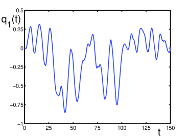
Figure 1: Interference factor $q_{1}(t)$ as a function of dimensionless time for the subcritical regime, with $b=0.25<b_{c}=0.282$.

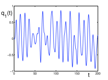
Figure 2: Interference factor $q_{1}(t)$ as a function of dimensionless time for the supercritical regime, with $b=0.5>b_{c}=0.282$.

Solving Eqs. (57) and (58) in the presence of the random perturbations, we take the initial conditions $s_{0}=-0.9,x_{0}=0$, which define the critical pumping parameter $b_{c}=0.282$. The results of the numerical solution for the interference factor (55), with $n=1$, are presented in Fig. 1 for the subcritical regime and in Fig. 2 for supercritical regime. It is sufficient to present only one interference factor, since the second is given by $q_{2}(t)=-q_{1}(t)$.

One can observe that the fluctuations of the interference factor are larger in the supercritical regime.

In conclusion, we have shown how the quantum probabilities for composite events, related to quantum measurements, can be defined. A special attention has been payed to the case of operationally uncertain measurements, when there appears an interference factor. We described how the average value of the interference factor can be estimated under rather general conditions. The necessity of entanglement in the considered prospect, as well as in the system state, for the appearance of interference has been stressed. An example of calculating the interference factor, employing the channel-state duality, for a trapped Bose-Einstein condensate with generated coherent modes, was demonstrated.

Financial supports from the Swiss National Foundation and from the Russian Foundation for Basic Research are acknowledged.

References

- [1] Keyl M 2002 Phys. Rep. 369 431
- [2] Birman J L, Nazmitdinov R G and Yukalov V I 2013 Phys. Rep. 526 1
- [3] von Neuman J 1955 Mathematical Foundations of Quantum Mechanics (Princeton: Princeton University)
- [4] Holevo A S 2011 Probabilistic and Statistical Aspects of Quantum Theory (Berlin: Springer)
- [5] Holevo A S and Giovanetti V 2012 Rep. Prog. Phys. 75 046001
- [6] Benioff P A 1972 J. Math. Phys. 13 908
- [7] Holevo A S 1973 J. Multivar. Anal. 3 337
- [8] Bohr N 1933 Nature 131 421
- [9] Bohr N 1933 Nature 131 457
- [10] Bohr N 1958 Atomic Physics and Human Knowledge New York: Wiley
- [11] Yukalov V I and Sornette D 2008 Phys. Lett. A 372 6867
- [12] Yukalov V I and Sornette D 2009 Entropy 11 1073
- [13] Yukalov V I and Sornette D 2009 Eur. Phys. J. B 71 533
- [14] Yukalov V I and Sornette D 2010 Adv. Complex Syst. 13 659
- [15] Yukalov V I and Sornette D 2011 Theor. Decis. 70 283
- [16] Yukalov V I and Sornette D 2013 Laser Phys. 23 105502
- [17] Birkhoff G and von Neumann J 1936 Ann. Math. 37 823
- [18] Gleason A M 1957 J. Math. Mech. 6 885
- [19] Huttner B, Muller A, Gautier J D, Zbinden H and Gisin N 1996 Phys. Rev. A 54 3783
- [20] Niestegge G 2004 J. Math. Phys. 45 4714
- [21] Bohr N 1913 Phil. Mag. 26 1
- [22] O’Connor K M and Wooters W K 2001 Phys. Rev. A 63 052302
- [23] Wang X 2001 Phys. Rev. A 64 012313
- [24] Arnesen M C, Bose S and Vedral V 2001 Phys. Rev. Lett. 87 017901
- [25] Zanardi P 2002 Phys. Rev. A 65 042101
- [26] Gittings J R and Fisher A J 2002 Phys. Rev. A 66 032305
- [27] Zanardi P and Wang X 2002 J. Phys. A 35 7947
- [28] Yukalov V I 2003 Phys. Rev. A 68 022109
- [29] Yukalov V I and Sornette D 2010 Phys. At. Nucl. 73 559
- [30] Yukalov V I, Yukalova E P and Bagnato V S 1997 Phys. Rev. A 56 4845
- [31] Yukalov V I, Yukalova E P and Bagnato V S 2000 Laser Phys. 10 26
- [32] Chin C, Grimm R, Julienne P and Tiesinga E 2010 Rev. Mod. Phys. 82 1225
- [33] Stimming H P, Mauser N J, Schmiedmayer J and Mazets I E 2011 Phys. Rev. A 83 023618
- [34] Yukalov V I, Yukalova E P 1996 J. Phys. A 29 6429
- [35] Yukalov V I, Yukalova E P and Sornette D 2013 Laser Phys. Lett. 10 115502