Using informative priors in the estimation of mixtures over time with application to aerosol particle size distributions

Abstract

The issue of using informative priors for estimation of mixtures at multiple time points is examined. Several different informative priors and an independent prior are compared using samples of actual and simulated aerosol particle size distribution (PSD) data. Measurements of aerosol PSDs refer to the concentration of aerosol particles in terms of their size, which is typically multimodal in nature and collected at frequent time intervals. The use of informative priors is found to better identify component parameters at each time point and more clearly establish patterns in the parameters over time. Some caveats to this finding are discussed.

, , , and m1Supported by the Academy of Finland through the Finnish Center of Excellence (project number 1118615).

1 Introduction

Aerosol particles have a direct and indirect impact on the earth’s climate. One of the most important physical properties of aerosol particles is their size, and the concentration of particles in terms of their size is referred to as the particle size distribution. An important characteristic of these data is that because aerosol particles are governed by formation and transformation processes they tend to form well distinguished modal features. Investigating these features provides an understanding of the dynamic behaviour of aerosol particles, their effect on the climate and their association with adverse health effects. This type of data is increasingly being measured on a regular basis, with the potential to provide more detailed information than, for example, measurements of particle mass concentrations such as PM10 or PM2.5, traditionally used for regulatory purposes [World Health Organization (2006)].

The most common approach for representing particle size distributions is by treating the size distribution at any time point as a set of individual typically normal distributions or modes [Hussein et al. (2005), Whitby, McMurry and Shanker (1991)]. In this formulation the estimation of particle size distributions is then analagous to a finite parametric mixture model problem at each time point.

While interest is in the representation of the particle size distribution as a mixture at each time point, it is also of interest to describe how this distribution evolves over time. To better understand aerosol dynamic processes, a feature of the measurements of particle size distributions is that they are often collected at regular points in time, and often at quite small time intervals (e.g., every 10 minutes). In this setting, parameters of the mixture model at each time point are likely to be correlated with neighboring time points and useful information about the parameters may be gained by incorporating this information in estimation.

The standard setting in which mixture models have been applied has largely been for independent random samples [Marin, Mengersen and Robert (2005)], but literature is developing for situations in which the data are spatially and/or temporally structured [Fernández and Green (2002), Green and Richardson (2002), Alston et al. (2007), Dunson (2006), Caron, Davy and Doucet (2007), Ji (2009)]. The development has largely been driven by the increasing availability of information in a wide variety of applications. An example includes analysing images (CAT scan) of sheep over time in which interest is in changes to the composition of fat, bone and tissue [Alston et al. (2007)]. In Ji (2009) interest is in cell fluorescent imaging tracking modelled using a dynamic spatial point process and a mixture representation for the different intensity functions observed.

For the air pollution example considered in this paper, we are interested in a mixture representation using a missing data approach, in which the components themselves can be interpreted as potential substrata of the data and for which further interest is in their behaviour over time. In particular, we are interested in the evolution of the parameters of the components over time, which in the case of the particle size distribution data is able to reveal important information about the number and change in size of particles for particular modes along with a measure of their variation. This information can then be used to better understand the potential variables affecting the dynamic behaviour of each mode (e.g., from local effects such as combustion from petrol and diesel vehicle engines, construction activity, wind speed, temperature, etc., and regional effects), which are likely to vary substantially between modes, and provide for a more accurate risk assessment of potential effects on adverse health outcomes (e.g., respiratory illnesses).

Popular recent approaches that allow for the correlated nature of the parameters in a mixture setting, both within and across epochs, include Dependent Dirichlet Process mixture models (DDPM) and (spatial) dynamic factor models (SDFM) [MacEachern (1999), Dunson (2006), Caron, Davy and Doucet (2007), Ji (2009), Strickland et al. (2011)]. While these approaches are appealing in the context of our case study, they do have some drawbacks. Importantly, interpretation of component parameters is less straightforward under the DDPM, and the SDFM typically requires relatively long time series [Strickland et al. (2011)]. An alternative that we consider here is the use of informative priors at each epoch in a finite parametric mixture setting, where the information required at each epoch is obtained from neighbouring epochs. This has appeal both in terms of a general Bayesian learning framework and in terms of interpretability of the mixture components and weights, which is important in our application. Moreover, while some of the methods developed for mixture models in the spatial setting [e.g., Fernández and Green (2002)] can potentially be adapted for use in a time series setting, the influence or choice of informative priors in a time series framework and the implications in different data environments have largely not been examined.

In this paper we explore three different informative priors for estimation of mixtures where the data are highly correlated, and all parameters in the mixture are allowed to vary. Different simulated data sets, with features similar to actual particle size distribution data, are used to highlight the influence of using informative priors and to identify situations where placing informative priors may not be beneficial.

The paper is structured as follows. In Section 2 we briefly describe particle size distributions and provide an illustration with actual data. In Section 3 we outline the finite parametric mixture model setup for a single time point and then outline the three approaches to estimation of a mixture model at multiple time points. Section 4 presents results on the performance of the approaches on several simulated data sets and actual data, and we conclude in Section 5 with some discussion and possibilities for further work.

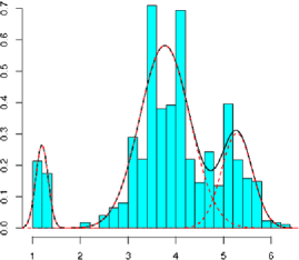
Figure 1: Histogram (normalised) of particle size data for a single time point [$x$-axis: $\log(D_{p}\mbox{ (nm)}$)]. The black (overall) and red (components) lines show the inferred density from estimation using RJMCMC.

2 Particle size distribution data

Figure 1 shows an example of particle size distribution data for one measurement or time point. The histogram shows the number of particles $N$ per cubic centimeter binned by particle size, with the horizontal axis representing the natural logarithm of the particle diameter in nm [$\log(D_{p})$]. The histogram is normalised, so that its total area equals 1.

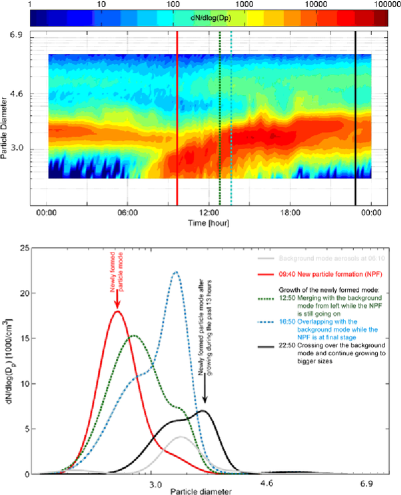
Figure 2: An illustration of a new particle formation event at a Boreal Forest site located in Southern Finland. (Top) the temporal variation of the particle size distribution and (bottom) selected particle size distributions showing the different stages of the newly formed particle mode. Particle diameter in (top) $y$-axis and (bottom) $x$-axis is on the $\log$ scale [i.e., $\log(D_{p}\mbox{ (nm)})$].

Because aerosol particles are charged, their size can be determined from their electrical mobility [McMurry (2000)] and a common instrument that utilises this principle is the Differential Mobility Particle Sizer (DMPS) [Aalto et al. (2001)].

In this study we present, as an example, the aerosol particle evolution before, during and after a new particle formation event at a Boreal Forest in Southern Finland (Figure 2). This data set was selected as it provides a wide ranging representation of modes for particle size distributions [Dal Maso et al. (2005)]. Because aerosol particles are governed by formation and transformation processes, they tend to form well distinguishable modal features. For example, during background conditions in the Boreal Forest the particle number size distribution of fine aerosols [diameter $<$2500 nm ($\log$, 7.82)] is bimodal: an Aitken mode [below 100 nm ($\log$, 4.60)] and an accumulation mode (over 100 nm). During a new particle formation event a new particle mode, which is commonly known as a nucleation mode, is formed in the atmosphere with geometric mean diameter below 25 nm ($\log$, 3.22). However, in the urban atmosphere aerosol particles are more dynamic because of the different types and properties of sources of aerosol particles and may show more than three modes. Typically the number concentrations of aerosol particles in the urban background can be as high as $5\times 10^{4}$ cm^-3 and close to a major road they often exceed $10^{5}$ cm^-3 [Kulmala et al. (2004)].

3 Methods

In this section we briefly describe the mixture model, outline a two stage approach to estimation of parameters over time, and describe three types of priors for temporal evolution of the parameters.

3.1 Mixture representation

The density of data ($y$) at a given time period may be represented by a finite parametric mixture model

$$p(y|\theta)=\sum_{j=1}^{k}\lambda_{j}f(y|\theta_{j}),$$ (1)

where $k$ is the number of components in the mixture, $\lambda_{j}$ represents the probability of membership of the $j$th component ($\sum_{j=1}^{k}\lambda_{j}=1$), and $f(y|\theta_{j}$) is the density function of component $j$ which has parameters $\theta_{j}$.

Let $i=1,\ldots,N$ indicate the observed data index. As component membership of the data is unknown, a computationally convenient method of estimation for mixture models is to use a hidden allocation process and introduce a latent indicator variable $z_{i}$, which is used along the lines of a missing variable approach to allocate observations $y_{i}$ to each component [Marin, Mengersen and Robert (2005)].

In this paper we adopt the common assumption of fitting normal distributions to aerosol particle size distribution data [Whitby and McMurry (1997)]. As PSD data are often measured with a definite lower and upper bound for the size of the particles, we introduce a slight modification and assume that the data follow a truncated normal distribution. As is commonly assumed, we take the data ($y$) to be the $\log$ of particle diameters (nm), and the parameters ($\theta_{j}$) for each component are the mean ($\mu_{j}$) and variance ($\sigma_{j}^{2}$). The number of components $k$ is also assumed to be unknown.

In the first stage of the temporal analysis, for each time period we implemented a reversible jump Markov chain Monte Carlo (RJMCMC) algorithm [Richardson and Green (1997)]. Although this algorithm is easily fit at a single time point, the use of RJMCMC for mixture models with temporal data requires significant preprocessing with respect to mixing coverage and convergence, as well as postprocessing to provide adequate summary statistics and between time component mapping.

As an alternative, we considered a two-stage approach. In the first stage, the number of components was estimated at each time point using RJMCMC. In the second stage, we fixed the number of components ($k$) to the maximum observed at any time point and independently estimated the parameters of the mixture model ($\mu$, $\sigma$ and $\lambda$) for each time point using a MCMC sampler algorithm. Details of the MCMC scheme used for the different cases are given below. As we do not observe all of the components in every time point, we allow component weights to be “effectively” zero [$\inf(\lambda_{t})=0.001$] if required [for details on the asymptotic behaviour of the posterior distribution using this approach see Rousseau and Mengersen (2011)]. Estimation of parameters of the components that are effectively “empty” under this criterion will then essentially be governed by their respective prior information. For the results to follow in Section 4 we thus only plot the parameters of components which are not “empty”.

Priors for the first stage of the analysis were

$$p(\mu_{j}) = \mathcal{N}\bigl{(}\xi,\kappa^{-1}\bigr{)},$$

$$p\bigl{(}\sigma_{j}^{2}\bigr{)} = \operatorname{IG}(\delta,\beta),$$

$$p(\beta) = \operatorname{Gamma}(g,h),$$

$$p(\lambda) = \operatorname{Dirichlet}(\alpha_{1},\ldots,\alpha_{k}),$$

$$p(k) = \operatorname{Uniform}(1,10),$$

where $\xi$, $\kappa$, $\delta$, $\alpha$, $\eta$, $g$, $h$ are hyperparameters.

For the second stage, priors were

$$p(\lambda) = \operatorname{Dirichlet}(\alpha_{1},\ldots,\alpha_{k}),$$

$$p\bigl{(}\mu_{j}|\sigma^{2}_{j}\bigr{)} = \mathcal{N}\biggl{(}\xi_{j},\frac{\sigma^{2}_{j}}{n_{j}}\biggr{)},$$ (2)

$$p\bigl{(}\sigma^{2}_{j}\bigr{)} = \operatorname{IG}\biggl{(}\frac{v_{j}}{2},\frac{s^{2}_{j}}{2}\biggr{)},$$

where again $\alpha_{j},\xi_{j},n_{j},v_{j}$ and $s_{j}$ are hyperparameters, detailed below. The prior for $\mu$ and $\sigma^{2}$ could alternatively be decoupled and expressed as in stage 1, but we did not see a noticeable difference in the results (Section 4) using either form. For the independent prior case, we use uninformative priors for $\mu$, $\sigma$ and $\lambda$.

3.2 Choice of temporal prior

In the second stage, four priors were considered for linking parameter values ($\mu,\sigma,\lambda$) over time. The first of these was the independent prior, in which the correlated nature of the data was ignored completely and parameters were independently estimated at each time point. The second, third and fourth were termed the “informed prior”, “penalised prior” and “hierarchical informed prior”, as described below.

3.2.1 Informed prior

In this approach we use the information provided from the previous time period as prior information for the current period. For the main results we focus on a simple case where posterior estimates from the previous period are used as prior information for the current period. We do this to illustrate the influence of a simple prior specification on the posterior estimates of parameters ($\theta$).

In the case of a mixture model using Gaussian distributions, we have three parameters ($\mu$, $\sigma$ and $\lambda$) for which we could utilise available prior information to aid in estimation. Preliminary investigation indicates that all three parameters are likely to show strong evidence of autocorrelation, so here we examine the effect of smoothing on each of these parameters.

For $p(\lambda)$, we allow $\alpha_{j}$ in equation (2) to reflect prior information about $\lambda_{j,t-1}$. Thus, we set $\alpha_{j}=\theta_{j}\bar{m}_{j,t-1}$, where $\bar{m}_{j,t-1}$ is the mean of the number of observations allocated to component $j$ in the previous time period, and $\theta_{j}$ is fixed at some value. An alternative is to impose a distribution on $\theta$, say, $\theta_{j}\sim\mathrm{U}(0,1)$ [or $\mathcal{N}(1,0.5$)], but we do not present the results for this approach in this paper.

For the specification of prior information for $\mu$ and $\sigma$, we set $\xi_{jt}=\mu_{j,t-1}$, $v_{j}=n_{j}/\sigma_{j,t-1}^{2}$ and $s_{j}=n_{j}$ [to ensure $p(\sigma^{2}_{jt})$ is centred on $\sigma^{2}_{j,t-1}$] and increase the value of $n_{j}$ from the value set for the independent case to reflect the degree of dependency for these parameters from the previous period.

3.2.2 Penalised prior

In this approach we base the priors at time $t$ on the aggregated information at all other time periods. This can be achieved by employing a reparameterisation of the prior to reflect the degree of dependency between parameters. Gustafson and Walker (2003) proposed a prior for $\lambda$ (in a different context) which can be used in our setting to downweight large changes in probabilities in successive time periods. Let $\underline{\lambda}=(\lambda_{jt},j=1,\dots,k,t=1,\dots,T)$, then $p(\underline{\lambda})$ is defined as

$$p(\underline{\lambda})\propto\operatorname{Dirichlet}(1,\dots,1)\exp\Biggl{(}-\frac{1}{\phi}\sum_{t=2}^{T}\|\underline{\lambda}_{t}-\underline{\lambda}_{t-1}\|^{2}\Biggr{)},$$ (3)

where smaller values of $\phi$ imply greater smoothing.

A potential advantage of using information about estimates both forwards and backwards in time is the additional information this may provide to guide parameter estimates in the current period. This may be most useful if large changes in the parameter estimates occur for single periods of time. For the purposes of comparison with Section 4.1, we compare the results of using a similar formulation for $\lambda$ in the informed prior approach (without smoothing on $\mu$ and $\sigma$).

Thus, prior distributions $p(\mu)$ and $p(\sigma)$ are set as for the independent approach [equation (2)].

For this formulation, we sampled from the posterior distribution of $\lambda$ using a rejection sampling approach outlined in Appendix A.

3.2.3 Hierarchical informed prior

In this approach an informative prior is placed at two different levels. The aim of allowing for different levels is to provide flexibility to the form in which prior information is given in the model. This flexibility may be needed in cases where the correlation structure can vary greatly over time: instead of imposing a smoothing structure directly on strongly varying parameters, we can provide a less restrictive smoothing through the hyperparameters.

For the hierarchical approach, we will focus on parameters $\mu$ and $\lambda$ as they are the main parameters of interest for the PSD data (see Section 4.4 and the Discussion). The hierarchical approach for $\mu$ is specified as

$$\mu_{jt} \sim \mathcal{N}\bigl{(}\phi_{jt},\varepsilon^{(d)}_{\mu}\bigr{)},$$

$$\phi_{jt} \sim \mathcal{N}\bigl{(}\phi_{j,t-1},\varepsilon^{(s)}_{\phi}\bigr{)},$$

where $\varepsilon^{(d)}_{\mu}$ and $\varepsilon^{(s)}_{\phi}$ are scalars, reflecting the variability of $\mu_{jt}$ and $\phi_{jt}$, respectively. Under this formulation, $\mu$ is used to estimate the mixture distribution at the level of the data, and $\phi$ represents the underlying correlation of $\mu$ over time [assuming in this case an AR(1) process]. In this setting, we can interpret the ratio $\varepsilon^{(s)}_{\phi}/\varepsilon^{(d)}_{\mu}$ as reflecting the amount of information we have about the underlying behaviour (signal) of $\mu$ in comparison to estimates at the level of the data (noise).

For the first time period ($t=1$), we set $\phi_{jt}=\mu_{jt}$. For estimation of $\mu$ and $\phi$, we use a Gibbs sampling scheme. For details see Appendix B.

For the parameter $\lambda$, the Dirichlet prior used in equation (2) for the independent model and the informed prior approach is a very common prior for discrete probabilities. A natural extension to the Dirichlet prior with a temporal component is to use its representation in terms of a Gamma distribution. However, the inflexibility of the Gamma distribution makes it difficult to construct a temporal structure to the Dirichlet prior. An alternative formulation of the Dirichlet in terms of the Beta distribution does not appear to provide greater flexibility.

Another alternative is to use a Logistic-Normal prior for $\lambda$, where

$$W_{t} \sim \mathcal{N}_{k-1}(X_{t},\Sigma_{d}),$$

$$\lambda_{jt} = \frac{\exp(W_{jt})}{\sum_{j=1}^{k-1}{\exp(W_{jt})}}$$

and where $X_{t}$ is the mean value (number of particles) at time period $t$.

Using this functional form, the parameterisation of $\lambda$ in terms of a multivariate normal distribution allows for a suitably flexible form in which to explore a hierarchical structure for this parameter. Such flexibility, in comparison to the Dirichlet distribution, has been investigated in a hierarchical approach for pooling of estimates across different sampling units [Hoff (2003)].

In a hierarchical setting and similar to the model used for $\mu$, we can further say that

$$X_{t} \sim \mathcal{N}_{k-1}(X_{t-1},\Sigma_{s}),$$

$$\gamma_{jt} = \frac{\exp(X_{jt})}{\sum_{j=1}^{k-1}{\exp(X_{jt})}},$$

where $\Sigma_{d}$ and $\Sigma_{s}$ reflect the variability of $W_{t}$ and $X_{t}$, respectively. Analogous to the above discussion for $\mu$, under this formulation the parameter $\lambda$ is used to estimate the mixture model at the level of the data, and $\gamma$ represents the underlying or smoothed behaviour of $\lambda$ over time, which may be prone to large fluctuations from the data.

For the simulation results and actual data to follow, we specify the diagonal entries of $\Sigma_{d}$ and $\Sigma_{s}$, and fix off-diagonal entries to be zero. For comparability with the hierarchical approach for $\mu$, and using similar notation for the smoothing parameters, we specify $\Sigma_{d}=\varepsilon^{(d)}_{\lambda}I_{d}$ and $\Sigma_{s}=\varepsilon^{(s)}_{\gamma}I_{d}$. The interpretation of $\varepsilon^{(d)}$ and $\varepsilon^{(s)}$ is then the same as before, but this time in terms of $\lambda$.

For estimation of $\lambda$ and $\gamma$ we use a Gibbs sampling scheme with a Metropolis Hastings step. For details see Appendix B. For identifiability both $W_{t}$ and $X_{t}$ are $k-1$ dimensional, and $\lambda_{k}=1-\sum_{j=1}^{k-1}\lambda_{j}$ (with the same identification used for $\gamma$).

In practice, it may be difficult to specify a priori the parameter values for $\varepsilon^{(d)}$ and $\varepsilon^{(s)}$, as little information about the variability of the parameters for the mixture components may be known. Estimation of these parameters also requires a choice to be made about the degree of smoothing required. For the purposes of this paper we focus on specifying the parameter values for $\varepsilon^{(d)}$ and $\varepsilon^{(s)}$, and explore briefly the effect on the results of varying these values. In the discussion we talk about this issue further. For now, one approach to specifying $\varepsilon^{(d)}$ may be to use the results from a RJMCMC approach used in the first stage, estimate or explore the variability of $\mu$ or $\lambda$ over time, and then use this information to set the parameter values for $\varepsilon^{(d)}$. The parameter value for $\varepsilon^{(s)}$ could be set as a smaller multiple of $\varepsilon^{(d)}$, and be varied to assess the influence of the results. Using the information from the results of the independent approach, for a fixed upper bound $k$ could also be used. Although there is extra computational time involved in running either approach in the first stage, such a strategy may prove useful in order to assess the influence of different prior information on the results.

3.3 Labelling issues

Where component parameters are themselves the subject of the analysis, an important and commonly encountered issue in Bayesian mixture modelling relates to the labelling of these parameters during the MCMC run. As the likelihood of a mixture is by definition multimodal, using exchangeable or noninformative priors can (and should) result in parameters moving freely over the parameter and component labelling space during sampling. (In theory, for a $k$ component mixture, $k!$ permutations of the labelling of the parameters are possible.) Estimation of functionals of these parameters (conditional on labelling) at the end of sampling is thus then problematic. Several empirical approaches to deal with this issue (commonly called “label switching”) have been proposed in the literature [Stephens (1997, 2000), Celeux, Hurn and Robert (2000), Frühwirth-Schnatter (2001, 2006), Jasra, Holmes and Stephens (2005), Marin, Mengersen and Robert (2005), Sperrin, Jaki and Wit (2010), Yao (2012)], generally by relabelling parameters in proximity to one of the $k!$ modal regions during the run [e.g., Frühwirth-Schnatter (2001)] or at the end of sampling [e.g., Stephens (1997)].

Under exchangeable or noninformative priors the main reason for label switching relates to a lack of identifiability of the mixture model (particularly with respect to enforcing a unique labelling). Given two component parameter sets $\theta_{j}$ and $\theta_{k}$, a finite mixture model is weakly identifiable if at least one element of $\theta_{j}$ and $\theta_{k}$ differs. For practical purposes then, the element that differs can be used to enforce a unique labelling. For exchangeable priors, in the sense that priors for $\theta_{j}$ and $\theta_{k}$ are the same, it is clear that there is a lack of identifiability.

In the case of using informative priors on $\theta_{j}$ and $\theta_{k}$, the issue of model identifiability is less clear. Although the use of different informative priors can help to separate $\theta_{j}$ and $\theta_{k}$, in practice, it will depend on the strength of the informative prior to separate at least one element of each parameter set. To our knowledge, there has been very little theoretical investigation of this issue. In practice, one can assess whether parameters are well separated by analysing the path of parameters over the sampling run and/or from plots of marginal densities. However, only part of the picture may be revealed by doing this. First, a relatively long sampling run is needed to allow the parameter to fully explore the space (perhaps many thousands of iterations). In the case of Gibbs sampling, the sampler may also become trapped in one of the modal regions [Celeux, Hurn and Robert (2000)]. Apart from the case of using a fully exchangeable prior, this second case is more difficult to identify in practice, as it can be unclear whether the Gibbs sampler is truly trapped or has found a uniquely labelled parameter space. A pragmatic solution could be to start the sampler from different values, although good starting locations can be difficult to determine in high-dimensional space. Alternative (and often more involved) solutions could be to: reparameterise and change the conditioning [Marin, Mengersen and Robert (2005)]; use tempering to facilitate more exploration [Celeux, Hurn and Robert (2000)]; and/or modify the Gibbs sampling proposal and acceptance [Celeux, Hurn and Robert (2000), Marin, Mengersen and Robert (2005)].

For both the independent and informed prior approaches outlined previously, it is possible to relabel the output using existing empirical approaches. In these cases, the posterior is updated sequentially across time and relabelling can take place during or at the end of each time period. In the results to be presented, we used the maximum a posteriori (MAP) estimate to select one of the $k!$ modal regions and chose either a distance-based measure on the space of parameters [Celeux, Hurn and Robert (2000)], or on the space of allocation probabilities [Stephens (1997), Marin, Mengersen and Robert (2005)] to relabel parameters in proximity to this region.

In the case of the penalised and hierarchical informed priors, a joint posterior that includes all components and all parameters over time is used and sampling updates occur globally over time. Relabelling of sampling output thus necessitates a permutation of labels for all time points together. Such a joint approach is similar in spirit to the Viterbi algorithm approach used in state space models [Godsill, Doucet and West (2001)], but the joint posterior in our case is different and would require further work outside the scope of this paper.

Using informative priors that are incompatible with the data can also force too many distinct components and lead to overfitting, which can in some cases lead to label switching. The potential for label switching could arise if two components with similar parameters are fitted where one component would suffice under the true model. As before, the similarity of the parameters could result in a lack of identifiability of the model. In using an informative prior there is also a model choice issue in terms of selecting the best model for the data, where “best” is defined, for example, as the most parsimonious model in terms of the smallest value of $k$. In practice, discrimination between the choice and use of informative priors can be made by fitting several mixture models to the data. Point-process representations of the estimated parameters from using a noninformative prior (such as Figure 8) can also offer a good visual guide as to the potential range and scope of the parameter space.

3.4 Accounting for binning and truncated data

Aerosol particle measurements are commonly recorded in the form of a number of distinct particle size ranges, or channels, the size and number of the channels being governed by the type and setup of the measurement instrument. For example, in the sampled data from Hyytiälä (see Figure 1 and Section 4.4), we observed 32 distinct size partitions (bins) covering the range from 3 nm to 650 nm.

Such coarsening of the data created by binning has an impact on density estimates and in a mixture context the number of components required to adequately model the data [Alston and Mengersen (2010)]. To address this, we add another step in the Gibbs sampler in which we simulate a new latent variable (say $x$) which is drawn from the believed underlying density of the data ($y$), in this case the fitted mixture model at current estimates of the parameters, at each iteration of the Gibbs sampler. As the sampling takes place within each bin, the simulation of the latent variable essentially involves sampling from a truncated Normal distribution for which there are a number of proposed approaches. For computational efficiency we used the slice-sampling approach of Robert and Casella (2004). For details of the approach and of the Gibbs sampler see Alston and Mengersen (2010). As the number of observations within each bin (and hence the latent sample size) is quite large, an extra step can be added after the latent variables are simulated in which the samples within each bin are divided into a number of sub-bins and computations in the Gibbs sampler proceed based on the new binned data. This can greatly speed up computations compared to using the full latent sample whilst reducing the coarsening of the data created by the original bins. In general, we found comparable results to the full latent sample by using 3 additional sub-bins for each original bin (in total 97 bins are used compared to the original 32 bins).

4 Results

In this section we present and assess the results using simulated data and then present the results of applying the approaches to particle size distribution data from Hyytiälä, Finland. We use the simulated data to test the impact of the different prior representations and the degree of smoothing. We first use an informative and penalised prior only on the weights ($\lambda$), and then assess the influence of using an informative prior on $\mu$ and $\sigma$ in order to assess the influence of using prior information for each parameter separately.

For the independent, informed and penalised prior approaches the results are based on 50,000 iterations with a burn-in period of 20,000 (i.e., the first 20,000 samples are discarded). Results using RJMCMC (used in the case study) are based on 200,000 iterations with a burn-in period of 100,000. Convergence was assessed by visual inspection and using the Gelman–Rubin statistic [Brooks and Gelman (1998)].

4.1 Simulated data

4.1.1 Data setup

We simulated data sets indicative of the type of behaviour of aerosol particle size distribution data observed at Hyytiälä, a Boreal Forest site in Southern Finland (SMEAR II) [Vesala et al. (1998)]. A particular feature of these particle size distribution data is both a growth in the mean and weight for some of the modes (components) and a decline in weight for others. Changes can also occur to the variance of the modes and at times they can follow a similar pattern to the weights over time.

We simulated data from two different cases. In the first case (D1), we simulated data which are highly correlated across time, a feature of particle size distribution data observed in practice for most time periods where measurements are commonly taken at small time intervals. This data set was also simulated with parameter estimates where at times the mixture is not well identified (component means and weights are not well separated). Of interest in this setting is the effect of using either the informed prior or penalised prior approach compared to the independent approach.

In practice, it is quite common to observe sudden large changes in the number of particles measured which may persist for a number of time periods. This is more often observed when there are relatively few particles for a particular size group, and more so for the smaller sized particles (an example of this type of data is examined in Section 4.4). Thus, for the second data set (D2) we simulated data for the first component where the weight for the smaller sized particles is quite volatile. For this data set the mixture is well identified. Further details and results are available in the supplementary material [Wraith et al. (2014)].

For both cases (D1) and (D2), we simulated data using three components on 32 distinct size partitions (bins) equally spaced (on the $\log$ scale) covering the range from 3 nm to 20 nm in particle diameter (on the $\log$ scale 1 to 3). The sample size for each time period is 1000 and the total number of time periods was 100. Further details of the sampling process for each case are provided in Section 4.2 and the supplementary material [Wraith et al. (2014), second data set (D2)].

For the results to follow, except as specified otherwise, for the independent, informed prior and penalised prior approaches, we set the hyperparameters to be $\xi=(1.5,3.5,5.0)$; $s^{2}_{t,j}=10$; $v_{t,j}=10/0.6^{2}$; and $n_{j}=2$, which were chosen to be weakly uninformative considering the range and size of the data. For the independent and informed prior approaches, the original Gibbs sampling output has been relabelled using a distance-based measure on the space of parameters [Celeux, Hurn and Robert (2000)] and also (as a check) on the allocation space [Stephens (1997), Marin, Mengersen and Robert (2005)].

4.2 Simulated data set (D1): Highly correlated data

4.2.1 Smoothing on $\lambda$

As shown in Figure 3 (black line), for the first data set (D1) we simulated data for the first component with a mean value increasing from 1.5 to 3.0, and weight increasing from 0.1 to 0.6 and then decreasing to 0.3, over time. Often a consequence of the growth in the first component is a decline in size and weight for the larger sized particles and this is reflected in the weight for the second component following an opposite pattern to the first component. For the third component, the weight increases from 0.1 to 0.3 over time. The parameters $\mu$ and $\lambda$ are simulated with some noise around the parameter values, and the sample size is 1000.

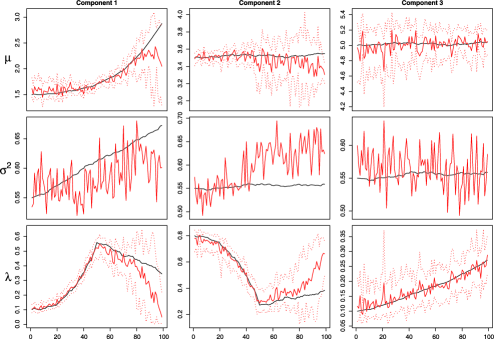
Figure 3: Results for simulated data set (D1) (highly correlated data) with growth and influx of new particles for component 1. Plot of estimated posterior mean for parameters [$\mu$ (top), $\sigma^{2}$ (middle) and $\lambda$ (bottom)] over time ($x$-axis) for independent approach: simulated data (black); independent (red); and 95% credible interval (dotted line). The columns represent the components (components 1 to 3).

Figure 3 also shows the results of using the independent approach. We see that at times the parameter estimates for the independent approach deviate from the actual data.

Figures 4 and 5 show the results for the informed prior and penalised prior compared to the actual data, respectively. In Figure 4, the results show the effect of varying the degree of smoothing on $\lambda$ for the informed prior using $\theta=(0.1,0.8,1.3)$. For the results of the penalised prior, we vary the degree of smoothing on $\lambda$ using $\phi=(0.04,0.08,0.12)$.

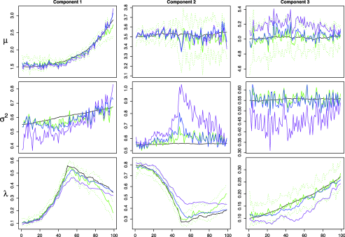
Figure 4: Results for simulated data set (D1) (highly correlated data) with growth and influx of new particles for component 1. Plot of estimated posterior mean for parameters [$\mu$ (top), $\sigma^{2}$ (middle) and $\lambda$ (bottom)] over time ($x$-axis) for informed prior approach: simulated data (black); Theta${}=0.1$ (green); Theta$={}$0.8 (blue); Theta${}=1.3$ (purple); and 95% credible interval (dotted line). The columns represent the components (components 1 to 3).

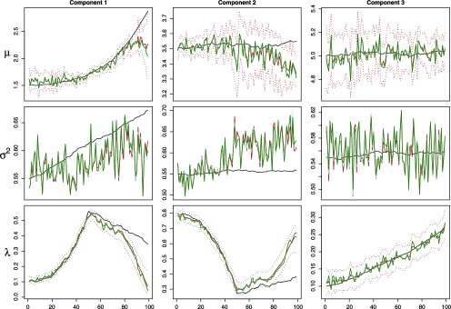
Figure 5: Results for simulated data set (D1) (highly correlated data) with growth and influx of new particles for component 1. Plot of estimated posterior mean for parameters [$\mu$ (top), $\sigma^{2}$ (middle) and $\lambda$ (bottom)] over time ($x$-axis) for penalised prior approach: simulated data (black); $\phi=0.04$ (brown); $\phi=0.08$ (light blue); $\phi=0.12$ (dark green); and 95% credible interval (dotted line). The columns represent the components (components 1 to 3).

In Figure 4, we can see that the parameter estimates for $\lambda$ for all three values of $\theta$ appear to closely follow the actual data, with the closest estimates to the actual data being for $\theta=0.8$ and 1.3. As we are only using an informed prior on the weights, the parameter estimates for $\mu$ and $\sigma$ appear to be quite variable over time compared to the actual data. However, the variability appears to be slightly less for these variables than for the independent approach (Figure 3) and closer to the actual data over time. Of interest is the closeness of the parameter estimates of $\mu$ and $\sigma$ for components 1 and 2, which more clearly follow the true growth occurring in component 1 and the stability over time for component 2 compared to that observed for the independent approach.

In Figure 5, the parameter estimates for the penalised prior approach appear to deviate slightly from the actual data for components 1 and 2. For the third component, the parameter estimates for the penalised prior approach follow the actual data with some noise. Overall, the results from the penalised prior approach are similar to the independent approach but with less variability over time.

4.2.2 Smoothing on $\mu$ and $\sigma$

We turn now to an assessment of the impact of using an informative prior for $\mu$ or $\sigma$ over time. We present results for the highly correlated data set, since this is the most sensitive of the simulated data as discussed above. Here we set $n_{j}=25$, $\xi_{jt}=\mu_{j,t-1}$, $v_{j}=200/\sigma_{j,t-1}^{2}$ and $s_{j}=200$.

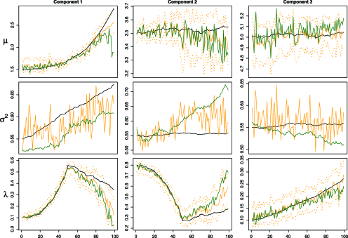
Figure 6: Results for simulated data set (D1) (highly correlated data) with growth and influx of new particles for component 1. Plot of estimated posterior mean for parameters [$\mu$ (top), $\sigma^{2}$ (middle) and $\lambda$ (bottom)] over time ($x$-axis) for informed prior approach: simulated data (black); smoothing on $\mu$ (orange); smoothing on $\sigma$ (dark green); and 95% credible interval (dotted line). The columns represent the components (components 1 to 3).

In Figure 6, the parameter estimates for the informative prior for $\mu$ appear to more closely follow the actual data than using an informative prior for $\sigma$. Although the parameter estimates for both approaches appear to be further away from the actual data than using an informative prior for $\lambda$, they do appear to be closer than under the independent approach.

4.2.3 Smoothing on $\mu$ and $\lambda$

Figure 7 shows the results of using an informative prior on both $\mu$ and $\lambda$. In this example, the results are similar to using an informative prior only on $\lambda$. Thus, depending on the objectives of the analysis, using an informative prior on both parameters may not be needed.

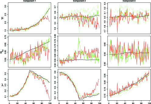
Figure 7: Results for simulated data set (D1) (highly correlated data) with growth and influx of new particles for component 1. Plot of estimated posterior mean for parameters [$\mu$ (top), $\sigma^{2}$ (middle) and $\lambda$ (bottom)] over time ($x$-axis) for approaches: simulated data (black); independent (red); smoothing on $\mu$ and $\lambda$ (green); and 95% credible interval (dotted line). The columns represent the components (components 1 to 3).

4.3 Simulated data set (D2): Noisy data

For the second simulated data set, where the weight for the smaller sized particles is quite volatile, the results of smoothing on $\mu$, $\sigma$ and $\lambda$ for the informed prior and penalised prior suggests that large adjustments to one parameter (e.g., from volatility in some time periods) are not supported unless compensatory measures can be taken by the other parameters. In contrast to these results, we do not see any large compensatory adjustments being made to parameters by using a hierarchically based informative prior for $\gamma$. Details are available in the supplementary material [Wraith et al. (2014)].

4.4 Case study

The data set studied here was taken from a measurement site at Hyytiälä, Finland; a plot of the measurements for the day selected is shown in Figure 2. This particular day was selected as it shows a new particle formation event occurring, whereby a new mode of aerosol particles appears with a significant influx of particles (as high as $10^{6}$ per cm³) with a geometric mean diameter ($<$10 nm), growing later into the Aitken (25–90 nm) or accumulation modes (100${}+{}$nm). In terms of a temporal mixture model setting, we will be able to assess the performance of the four prior specifications outlined previously as new components are introduced and both a growth in the mean and weight for those components are observed.

The data from Hyytiälä consists of measurements which were taken every 10 minutes (144 time periods) and for each time period in the form of 32 distinct size partitions (bins) equally scaled (on the $\log$ scale) covering the range of 3 nm to 650 nm (on the $\log$ scale 1 to 6.5).

As outlined in Section 3, the first stage of our approach is to apply RJMCMC to each time period. These results are then used to guide the choice of the number of components and initial parameter estimates for the second stage analysis, in which temporally correlated priors are used to model the evolution of the mixture parameters over time. Figure 8 shows the results of the first stage of the algorithm, with a plot of the posterior mean estimates for $\mu_{jt}$ at each time point $t$ (bottom panel), with the size of the circles indicating the corresponding weight $\lambda_{jt}$. The average number of components estimated with the highest probability over the day was four; the minimum number of components was one, and the maximum number of components was five (see top panel of Figure 8).

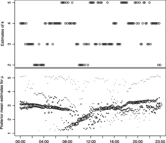
Figure 8: (Top) plot of estimates of $k$ (posterior median) from RJMCMC algorithm over time (every 10 minutes) (Hyytiälä). (Bottom): plot of posterior mean estimates for $\mu_{j}$ [$\log(D_{p}\mbox{ (nm)}$)] from RJMCMC algorithm over the same time period. Stage 1 of analysis for temporal evolution of parameters. The size of the circles is proportional to the weight ($\lambda_{jt}$) corresponding to $\mu_{jt}$.

For the second stage, we fixed the number of components to be five with the initial mean values equally spaced across the range of possible diameter values [$\xi=(1.1,2.0,3.0,4.0,5.0)$] and $\kappa=10$. Figure 9 shows the results of estimation using the independent approach (original output has been relabelled using a distance-based measure on the space of parameters [Celeux, Hurn and Robert (2000)]; similar results were obtained by relabelling on the allocation space [Stephens (1997), Marin, Mengersen and Robert (2005)]).

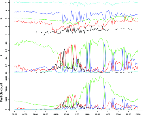
Figure 9: Plot of estimated posterior mean for parameters over time for actual data. Independent approach. Posterior mean estimates for $\mu$ [(top) $\log(D_{p}\mbox{ (nm)}$)], $\lambda$ (middle) and particle count (per cm³) (bottom). Stage 2 of the analysis for the evolution of parameters. Measurements taken every 10 minutes. Colours indicate the components to which parameter estimates belong. (The parameter estimates for the first component are black, parameters for the second component are red, for the third component they are green, etc.) Note: only components where $\lambda>0.01$ are plotted.

Due to the large number of particles (per cm³) observed over the day (see Figure 2), the results of estimation using the informed prior approach for $\mu$ and/or $\lambda$ are very similar to the results of the independent approach, so are not shown here. As we are interested in the effect of using an informative prior in this context, we rescale the number of particles by a factor of $10$ and assess the results. The median number of particles over the course of the day is then 6893, reaching a maximum of 17,740. Using this rescaling of the data, the results of the independent approach are the same as shown in Figure 9.

Figure 10 shows the results of estimation using the informed prior approach for $\mu$ and $\lambda$. For these results, $\theta=0.2$, $n_{j}=15$ and $\xi_{jt}=\mu_{j,t-1}$, which provides for a moderately informative prior across time. Similar results were obtained using the hierarchical model with similar strength of prior information. Of interest to note is that in the original output we did not see any evidence of label switching within the gibbs sampling runs. Although there is some evidence of instability between 12:00 and 13:00 for the weight ($\lambda_{j}$) of two of the components (newly formed and background particles), this appears to be due to instability in the data (see Figure 8), with the means of these components remaining reasonably well separated during this period.

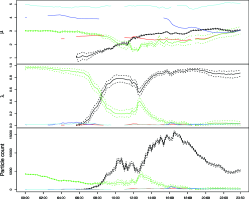
Figure 10: Plot of estimated parameters over time for actual data. Informed prior approach for $\mu$ and $\lambda$. Posterior mean estimates for $\mu$ [(top) $\log(D_{p}\mbox{ (nm)}$)], $\lambda$ (middle) and particle count (per cm³) (bottom) and 95% credible interval (dotted line). Stage 2 of the analysis for the evolution of parameters. Measurements taken every 10 minutes. Colours indicate the components to which parameter estimates belong. (The parameter estimates for the first component are black, parameters for the second component are red, for the third component they are green, etc.) Note: only components where $\lambda>0.01$ are plotted.

Compared to the results from the independent approach (Figure 9), the results from the informed prior approach for $\mu$ and $\lambda$ suggest a clear pattern for both over the course of the day. In particular, and of interest to aerosol physicists, is the clear growth pattern shown for the mean of the first component representing the smaller sized particles. The results indicate that these particles grow from approximately 1.40 (4 nm) to 3.0 (20 nm) in diameter on the natural $\log$ scale (or in nanometers).

The path of the parameters for the first component (black) is less clear using the independent approach, principally as a result of the newly formed smaller particles merging into the component representing the background particles (green). There is also some evidence of instability in the labelling across time, which is natural given the absence of temporal information in the prior.

We note that different representations of this data are possible depending on prior assumptions. If we relax the assumed moderate correlation of the new and background particles, then there is less separation between the component associated to the newly formed particles and to that of the background particles, similar to the results we see for the independent approach. Ideally, more information is needed to model these data; this could take the form of greater assumptions about the underlying stochastic process and the possible inclusion of external factors (e.g., meteorological data) impacting/influencing the observed process. We discuss this issue more in the following section.

5 Discussion

In this paper we explored the problem of estimating Bayesian mixture models at multiple time points. Under different situations, approaches that employ information about neighbouring time points compared favourably to results based on an independent approach. By including additional temporal information about parameters for correlated time periods, we may be able to better identify individual components at each time point. As an aid for inference, we may also be able to obtain smoother parameter estimates over time and from this be able to clearly establish patterns or identify anomalies from the data.

The results highlight a number of observations about mixture representations at multiple time points. First, analysis of the evolution of parameters of a mixture over multiple time points highlights the large degree of dependency that exists between component parameters. Changes to a parameter in one component may flow on to the parameter in a nearby component. Depending on the context of the study, we can anticipate this dependency to be more readily apparent for the weight parameters, but we found similar dependencies to exist for other parameters. The second is the need to be mindful that the same parameter in one component may have a different correlation structure over time to the same parameter in another component. In the context of particle size distribution data, we often observed greater volatility in estimates for the smaller particles compared to the larger sized particles and so at times the correlation structure of the parameters between these respective components appeared to be quite different.

A possible effect of using informative priors in this context is to impose a prior not supported by the data or to impose a temporal correlation structure where such a structure does not exist, and thereby cause unnecessary adjustments to other parameters. We observed this most clearly in the results from the simulated data where at times the data was quite noisy. For this data set, using an informative prior for a parameter, which supported large adjustments away from the actual data, resulted in large compensatory adjustments being made not only by other parameters within the same component, but also to parameters in neighbouring components. The easy solution may be to use an appropriate correlation structure for components, but of course this may not always be known a priori.

A further result of the dependency that can exist between parameters of components and within component parameters is that the inclusion of correlation information to aid in the identifiability of the mixture may not be required for all parameters or, alternatively, all components. In the context of a mixture with a small number of components, we may only need to provide more information about one parameter for an influential component in order to separate out the influence of competing components. This result will also be useful if the correlation structure for one parameter or parameters for one component are more readily known. In the context of a mixture of Gaussians, we generally found that an informative prior was only needed on $\mu$ or $\lambda$ or possibly both. This result could well be context specific and influenced by any reliance on the means for defining (in terms of size) and ordering of components. The choice of which parameter to use more information may also be guided by whether it is a parameter of interest for inference as demonstrated in analysis of the case study where most interest was in the behaviour of both $\mu$ and $\lambda$ over time. In this case, and in general, one must be careful in the analysis of selected parameters, as it can largely be a conditional analysis in view of the behaviour of other possible cross-correlated parameters within the same component and between components.

In the hierarchical informed prior approach the influence of the informative prior at the two levels was specified by parameters $\varepsilon^{(d)}$ (low level) and $\varepsilon^{(s)}$ (high level), and the values assigned to these parameters are critical in carrying information about the correlation structure of the parameter of interest. In this paper, we decided to choose parameter values based on prior belief in the correlation structure of the data; alternatively, these parameters could be estimated. To this effect, a number of approaches are available for estimation [West and Harrison (1997), Fahrmeir, Kneib and Lang (2004)]. However, in order to estimate $\varepsilon^{(d)}$ and $\varepsilon^{(s)}$, we still face a choice as to the degree of penalisation or smoothing of the parameter in light of the apparent variability in the data. This is a common issue in temporal and spatial modelling in general.

While many of the above difficulties may seem to be avoided if smoothing approaches are applied retrospectively on parameter estimates from an independent mixture model, this type of analysis may largely ignore the true mapping of components or the path of parameters over time. From the results of the simulated data, the large degree of dependency that we observe between the parameters of a mixture over time suggests that including temporal information to better identify one of the parameters at a single time point can flow on to affect other parameters. This could change inference about both the mixture representation at a point in time and also the behaviour of mixture parameters over time.

In general, one of the potential difficulties in using an informative prior approach to smooth parameter estimates over time is the variable degree of influence the prior may have in the posterior. If the primary objective is to obtain smoothed parameter estimates over time, larger sample sizes and noisiness of the data at times may warrant increasingly restrictive priors. In such cases where the objective might be to downplay the influence of the data, a number of alternative approaches to increase the influence of prior information can be used [Ibrahim, Chen and Sinha (2003)]. In all cases, it is valuable to undertake a sensitivity analysis in order to assess the effect of the prior. Such an analysis should include the independent prior as a baseline comparison.

A further limitation of the approach outlined is that it is computationally expensive. Most of this expense is experienced in the first stage of the analysis (which can be skipped in the presence of good prior knowledge of the parameter space). For estimation of PSD data over one day using 144 time points, the running time of the RJ approach with 200,000 iterations was approximately 3 hours using an Intel Centrino 2 processor 2.80 GHz. In comparison, the second stage approach using 50,000 iterations took approximately one hour. Such computational expense quickly becomes burdensome if analyses is required for several days or, indeed, several weeks. Of course, the use of the first stage for subsequent days may not be required, considerably reducing the computational time involved.

Although we have focussed on developing a hierarchical approach for parameters $\mu$ and $\lambda$, we could equally apply the same approach to consider estimation of $\sigma$. Such an approach may be to consider a half-$t$ distribution which has previously been used in similar hierarchical settings [Gelman (2006)].

The hierarchical approach considered here can be readily generalised to include covariates. Moreover, through the flexibility of assuming a logistic normal distribution on the weights, we can better explore and estimate transitory movements between components.

In some situations it may be of interest to combine components and allow components to share a common grouping. This could be of interest where some components are only needed to account for the skewness of a larger component or to allow an analysis based on a mixture representation with fewer components of most interest. Although this grouping of components could be undertaken retrospectively, it may also be interesting to see the effects such a grouping has upon estimation of the parameters and their evolution over time.

For estimation of aerosol particle size distributions, the dynamics of the aerosol process and the complexity of the influences on particle concentration and size demand the use of approaches which utilise as much information from the data as possible. To this end, the inclusion of temporal information may be helpful.

Appendix A Penalised prior

In this section we outline the rejection sampling algorithm for $\lambda$ proposed by Gustafson and Walker (2003) for the penalised prior approach:

Prior

$$p(\underline{\lambda})\propto\operatorname{Dirichlet}(1,\ldots,1)\exp\Biggl{(}-\frac{1}{\phi}\sum_{t=2}^{T}\|\underline{\lambda}_{t}-\underline{\lambda}_{t-1}\|^{2}\Biggr{)}.$$ (7)

Posterior

$$p(\underline{\lambda}|\phi,m)$$

$$\qquad\propto\prod_{j=1}^{k}\Biggl{\{}\prod_{t=1}^{T}\operatorname{Dirichlet}(m_{jt}+1)\mathrm{I}(\lambda_{jt})\Biggr{\}}\exp\Biggl{(}-\frac{1}{\phi}\sum_{t=2}^{T}\|\underline{\lambda}_{t}-\underline{\lambda}_{t-1}\|^{2}\Biggr{)}.$$

Gustafson and Walker (2003) suggest sampling $\lambda_{jt}/s$ from a $\operatorname{Beta}(m_{jt}+1$, $m_{kt}+1)$ distribution and accepting when $U\leq g_{1}(\lambda_{jt})/g_{2}(\lambda_{jt})$ ($U\sim\mathrm{U}(0,1)$), where

$$g_{1}(\lambda_{jt}) = \lambda_{jt}^{m_{jt}}(s-\lambda_{jt})^{m_{kt}}\mathrm{I}(\lambda_{t})$$

$${}\times\exp\bigl{[}-\phi^{-2}\bigl{\{}(\lambda_{jt}-\lambda_{j,t-1})^{2}+\bigl{(}\lambda_{jt}-(s-\lambda_{j,t-1})\bigr{)}^{2}$$

$$\hskip 62.0pt{}+(\lambda_{jt}-\lambda_{j,t+1})^{2}+\bigl{(}\lambda_{jt}-(s-\lambda_{k,t+1})\bigr{)}^{2}\bigr{]}\bigr{)}$$

and

$$g_{2}(\lambda_{jt}) = \lambda_{jt}^{m_{jt}}(s-\lambda_{jt})^{m_{kt}}\mathrm{I}(\lambda_{t})$$

$${}\times\exp\bigl{[}-\phi^{-2}\bigl{\{}\bigl{(}\lambda^{*}-\lambda_{j,t-1}\bigr{)}^{2}+\bigl{(}\lambda^{*}-(s-\lambda_{j,t-1})\bigr{)}^{2}$$

$$\hskip 62.0pt{}+\bigl{(}\lambda^{*}-\lambda_{j,t+1}\bigr{)}^{2}+\bigl{(}\lambda^{*}-(s-\lambda_{k,t+1})\bigr{)}^{2}\bigr{]}\bigr{)},$$

where

$$\quad\lambda^{*}=\max\bigl{\{}0,\min\bigl{\{}\tfrac{1}{4}(\lambda_{j,t-1}+s-\lambda_{k,t-1}+\lambda_{j,t+1}+s-\lambda_{k,t+1}),s\bigr{\}}\bigr{\}},$$ (11)

$s=\lambda_{jt}+\lambda_{kt}$ and $g_{1}(\lambda_{jt})\leq g_{2}(\lambda_{jt})$. Here $I(\lambda_{t})$ is an indicator function equal to 1 when $\lambda_{t}\in[0,1]^{2}$ and 0 otherwise.

Appendix B Details of MH Gibbs sampler for hierarchical model

Hierarchical model for $\mu$

Update $z$, $\beta$, $\lambda$, $\sigma^{2}$ as in the independent approach.

Update $\phi$ and $\mu$ by sampling from the conditionals,

$$\phi_{jt}|\cdot \sim \mathcal{N}\biggl{(}\frac{\varepsilon^{(d)}\phi_{j,t-1}+\varepsilon^{(s)}\mu_{jt}}{\varepsilon^{(d)}+\varepsilon^{(s)}},\frac{1}{(\varepsilon^{(d)})^{-1}+(\varepsilon^{(s)})^{-1}}\biggr{)},$$

$$\mu_{jt}|\cdot \sim \mathcal{N}\biggl{(}\frac{\phi_{jt}+m_{j}\bar{y_{j}}\varepsilon^{(d)}\sigma_{jt}^{-2}}{\varepsilon^{(d)}m_{j}\sigma_{jt}^{-2}+1},\frac{\varepsilon^{(d)}}{(\varepsilon^{(d)}m_{j}\sigma_{jt}^{-2}+1)}\biggr{)}.$$

Hierarchical model for $\lambda$

Update $z$, $\beta$, $\mu$, $\sigma^{2}$ as in the independent approach. Update $\gamma_{t}$ by sampling from the conditional,

$$X_{t} \sim \mathcal{N}_{k-1}\biggl{(}\frac{\Sigma_{d}^{-1}W_{t}+\Sigma_{s}^{-1}X_{t-1}}{\Sigma_{d}^{-1}+\Sigma_{s}^{-1}},\frac{1}{\Sigma_{d}^{-1}+\Sigma_{s}^{-1}}\biggr{)},$$

$$\gamma_{jt} = \frac{\exp(X_{jt})}{\sum_{j=1}^{k-1}{\exp(X_{jt})}},$$

where $X_{kt}=0$.

Update $\lambda_{t}$ using a Metropolis Hastings step.

Sample from $W_{t}\sim\mathcal{N}_{k-1}(X_{t},\sigma^{2}_{p}I)$, where $\lambda_{jt}=\exp(W_{jt})/\sum_{j=1}^{k-1}\exp(W_{jt})$ and $\sigma^{2}_{p}$ is the variance of the proposal.

Let $W_{k1}=0$ and for $t=2$, $W_{j2}=\log(\overline{m}_{j1}/\overline{m}_{k1})$, where $\overline{m}_{j1}$ is the mean number of observations allocated to component $j$ in the previous time period (under the independent approach).

References

- Aalto et al. (2001) {barticle}[author] \bauthor\bsnmAalto, \bfnmP.\binitsP., \bauthor\bsnmHämeri, \bfnmK.\binitsK., \bauthor\bsnmBecker, \bfnmE.\binitsE., \bauthor\bsnmWeber, \bfnmR.\binitsR., \bauthor\bsnmSalm, \bfnmJ.\binitsJ., \bauthor\bsnmMakela, \bfnmJ. M.\binitsJ. M., \bauthor\bsnmHoell, \bfnmC.\binitsC., \bauthor\bsnmO’Dowd, \bfnmC.\binitsC., \bauthor\bsnmKarlsson, \bfnmH.\binitsH., \bauthor\bsnmHansson, \bfnmH. C.\binitsH. C., \bauthor\bsnmVakeva, \bfnmM.\binitsM., \bauthor\bsnmKoponen, \bfnmI. K.\binitsI. K., \bauthor\bsnmBuzoris, \bfnmG.\binitsG. and \bauthor\bsnmKulmala, \bfnmM.\binitsM. (\byear2001). \btitlePhysical characterization of aerosol particles during nucleation events. \bjournalTellus \bvolume53 \bpages344–358. \bptokimsref \endbibitem
- Alston and Mengersen (2010) {barticle}[mr] \bauthor\bsnmAlston, \bfnmC. L.\binitsC. L. and \bauthor\bsnmMengersen, \bfnmK. L.\binitsK. L. (\byear2010). \btitleAllowing for the effect of data binning in a Bayesian normal mixture model. \bjournalComput. Statist. Data Anal. \bvolume54 \bpages916–923. \biddoi=10.1016/j.csda.2009.10.003, issn=0167-9473, mr=2580926 \bptokimsref \endbibitem
- Alston et al. (2007) {barticle}[mr] \bauthor\bsnmAlston, \bfnmC. L.\binitsC. L., \bauthor\bsnmMengersen, \bfnmK. L.\binitsK. L., \bauthor\bsnmRobert, \bfnmC. P.\binitsC. P., \bauthor\bsnmThompson, \bfnmJ. M.\binitsJ. M., \bauthor\bsnmLittlefield, \bfnmP. J.\binitsP. J., \bauthor\bsnmPerry, \bfnmD.\binitsD. and \bauthor\bsnmBall, \bfnmA. J.\binitsA. J. (\byear2007). \btitleBayesian mixture models in a longitudinal setting for analysing sheep CAT scan images. \bjournalComput. Statist. Data Anal. \bvolume51 \bpages4282–4296. \biddoi=10.1016/j.csda.2006.05.013, issn=0167-9473, mr=2364445 \bptokimsref \endbibitem
- Brooks and Gelman (1998) {barticle}[mr] \bauthor\bsnmBrooks, \bfnmStephen P.\binitsS. P. and \bauthor\bsnmGelman, \bfnmAndrew\binitsA. (\byear1998). \btitleGeneral methods for monitoring convergence of iterative simulations. \bjournalJ. Comput. Graph. Statist. \bvolume7 \bpages434–455. \biddoi=10.2307/1390675, issn=1061-8600, mr=1665662 \bptokimsref \endbibitem
- Caron, Davy and Doucet (2007) {binproceedings}[author] \bauthor\bsnmCaron, \bfnmF.\binitsF., \bauthor\bsnmDavy, \bfnmM.\binitsM. and \bauthor\bsnmDoucet, \bfnmA.\binitsA. (\byear2007). \btitleGeneralized Polya urn for time-varying Dirichlet process mixtures. In \bbooktitle23rd Conference on Uncertainty in Artificial Intelligence (UAI’2007). \bpublisherVancouver, \blocationCanada. \bptokimsref \endbibitem
- Celeux, Hurn and Robert (2000) {barticle}[mr] \bauthor\bsnmCeleux, \bfnmGilles\binitsG., \bauthor\bsnmHurn, \bfnmMerrilee\binitsM. and \bauthor\bsnmRobert, \bfnmChristian P.\binitsC. P. (\byear2000). \btitleComputational and inferential difficulties with mixture posterior distributions. \bjournalJ. Amer. Statist. Assoc. \bvolume95 \bpages957–970. \biddoi=10.2307/2669477, issn=0162-1459, mr=1804450 \bptokimsref \endbibitem
- Dal Maso et al. (2005) {barticle}[author] \bauthor\bparticleDal \bsnmMaso, \bfnmM.\binitsM., \bauthor\bsnmKulmala, \bfnmM.\binitsM., \bauthor\bsnmRiipinen, \bfnmI.\binitsI., \bauthor\bsnmWagner, \bfnmR.\binitsR., \bauthor\bsnmHussein, \bfnmT.\binitsT., \bauthor\bsnmAalto, \bfnmP. P.\binitsP. P. and \bauthor\bsnmLehtinen, \bfnmK. E. J.\binitsK. E. J. (\byear2005). \btitleFormation and growth of fresh atmospheric aerosols: Eight years of aerosol size distribution data from SMEAR II, Hyytiala, Finland. \bjournalBoreal Env. Res. \bvolume10 \bpages323–336. \bptokimsref \endbibitem
- Dunson (2006) {barticle}[author] \bauthor\bsnmDunson, \bfnmD. B.\binitsD. B. (\byear2006). \btitleBayesian dynamic modelling of latent trait distributions. \bjournalBiostatistics \bvolume7 \bpages551–568. \bptokimsref \endbibitem
- Fahrmeir, Kneib and Lang (2004) {barticle}[mr] \bauthor\bsnmFahrmeir, \bfnmLudwig\binitsL., \bauthor\bsnmKneib, \bfnmThomas\binitsT. and \bauthor\bsnmLang, \bfnmStefan\binitsS. (\byear2004). \btitlePenalized structured additive regression for space-time data: A Bayesian perspective. \bjournalStatist. Sinica \bvolume14 \bpages731–761. \bidissn=1017-0405, mr=2087971 \bptokimsref \endbibitem
- Fernández and Green (2002) {barticle}[mr] \bauthor\bsnmFernández, \bfnmCarmen\binitsC. and \bauthor\bsnmGreen, \bfnmPeter J.\binitsP. J. (\byear2002). \btitleModelling spatially correlated data via mixtures: A Bayesian approach. \bjournalJ. R. Stat. Soc. Ser. B Stat. Methodol. \bvolume64 \bpages805–826. \biddoi=10.1111/1467-9868.00362, issn=1369-7412, mr=1979388 \bptokimsref \endbibitem
- Frühwirth-Schnatter (2001) {barticle}[mr] \bauthor\bsnmFrühwirth-Schnatter, \bfnmSylvia\binitsS. (\byear2001). \btitleMarkov chain Monte Carlo estimation of classical and dynamic switching and mixture models. \bjournalJ. Amer. Statist. Assoc. \bvolume96 \bpages194–209. \biddoi=10.1198/016214501750333063, issn=0162-1459, mr=1952732 \bptokimsref \endbibitem
- Frühwirth-Schnatter (2006) {bbook}[mr] \bauthor\bsnmFrühwirth-Schnatter, \bfnmSylvia\binitsS. (\byear2006). \btitleFinite Mixture and Markov Switching Models. \bpublisherSpringer, \blocationNew York. \bidmr=2265601 \bptokimsref \endbibitem
- Gelman (2006) {barticle}[mr] \bauthor\bsnmGelman, \bfnmAndrew\binitsA. (\byear2006). \btitlePrior distributions for variance parameters in hierarchical models. \bjournalBayesian Anal. \bvolume1 \bpages515–533 (electronic). \bidmr=2221284 \bptnotecheck related\bptokimsref \endbibitem
- Godsill, Doucet and West (2001) {barticle}[mr] \bauthor\bsnmGodsill, \bfnmSimon\binitsS., \bauthor\bsnmDoucet, \bfnmArnaud\binitsA. and \bauthor\bsnmWest, \bfnmMike\binitsM. (\byear2001). \btitleMaximum a posteriori sequence estimation using Monte Carlo particle filters. \bjournalAnn. Inst. Statist. Math. \bvolume53 \bpages82–96. \biddoi=10.1023/A:1017968404964, issn=0020-3157, mr=1777255 \bptokimsref \endbibitem
- Green and Richardson (2002) {barticle}[mr] \bauthor\bsnmGreen, \bfnmPeter J.\binitsP. J. and \bauthor\bsnmRichardson, \bfnmSylvia\binitsS. (\byear2002). \btitleHidden Markov models and disease mapping. \bjournalJ. Amer. Statist. Assoc. \bvolume97 \bpages1055–1070. \biddoi=10.1198/016214502388618870, issn=0162-1459, mr=1951259 \bptokimsref \endbibitem