The ballistic transport instability in Saturn’s rings III: numerical simulations

Abstract

Saturn’s inner B-ring and its C-ring support wavetrains of contrasting amplitudes but with similar length scales, 100—1000 km. In addition, the inner B-ring is punctuated by two intriguing ‘flat’ regions between radii 93,000 km and 98,000 km in which the waves die out, whereas the C-ring waves coexist with a forest of plateaus, narrow ringlets, and gaps. In both regions the waves are probably generated by a large-scale linear instability whose origin lies in the meteoritic bombardment of the rings: the ballistic transport instability. In this paper, the third in a series, we numerically simulate the long-term nonlinear evolution of this instability in a convenient local model. Our C-ring simulations confirm that the unstable system forms low-amplitude wavetrains possessing a preferred band of wavelengths. B-ring simulations, on the other hand, exhibit localised nonlinear wave ‘packets’ separated by linearly stable flat zones. Wave packets travel slowly while spreading in time, a result that suggests the observed flat regions in Saturn’s B-ring are shrinking. Finally, we present exploratory runs of the inner B-ring edge which reproduce earlier numerical results: ballistic transport can maintain the sharpness of a spreading edge while building a ‘ramp’ structure at its base. Moreover, the ballistic transport instability can afflict the ramp region, but only in low-viscosity runs.

1 Introduction

Planetary rings of low and intermediate optical depth are vulnerable to the ballistic transport instability (BTI) which issues from the continual bombardment of ring particles by hypervelocity micrometeoroids. Ejecta released via these impacts reaccrete on to the ring at various radii, and thus redistribute mass and angular momentum (Durisen 1984, Ip 1984, Lissauer 1984). A small positive perturbation in surface density will change the ring’s local transport properties, and if the overdense region releases less material than it can absorb relatively, then it will grow and an instability results (Durisen 1995, Latter et al. 2012, hereafter Paper 1). The BTI favours long lengthscales $l_{\text{th}}\sim 10-10^{3}$ km and long timescales $t_{e}\sim 10^{5}-10^{7}$ yr. Thus the 100-km waves in the inner B-ring (between radii 93,000 and 98,000 km) and the 1000-km undulations in the C-ring (between 77,000 and 86,000 km) are possible manifestations of its nonlinear development (Figs 13.17 and 13.13 in Colwell et al. 2009, Charnoz et al. 2009 ).

This is the third paper in a series exploring the dynamics of the BTI and its generation of wave-like structure. The first paper presented a convenient local model with which to study the problem and worked through the BTI’s linear theory (Paper 1). The second paper established semi-analytically that the instability could sustain families of nonlinear travelling wavetrains (Latter et al. 2013, herafter Paper 2). For C-ring parameters, these waves saturate at low amplitude. For B-ring parameters, the ring exhibits bistability, with the system falling into one of two linearly stable states: the background homogeneous state (a ‘flat zone’) or a large-amplitude wave state (a ‘wave zone’). Both results are consistent with Cassini data and strengthen the connection between the observed wave features and the BTI.

In this paper, our earlier results are verified and extended with time-dependent simulations. Our numerical algorithm exploits the convolution form of the ballistic transport integrals and, as a result, can easily evolve the system on extremely long timescales $\sim 1000\,t_{e}$ and lengthscales $\sim 100\,l_{\text{th}}$. We subsequently calculate structure formation in three contexts: (a) low-optical depth models of the C-ring, (b) bistable models of the B-ring, and (c) the spreading and structure of a sharp edge.

The low-optical depth simulations fulfil most of the expectations of Paper 2. After an initial period of wave competition, the system settles upon a linearly stable low-amplitude wavetrain that fills the domain. Our simulations, however, possess translational symmetry, a special constraint not shared by the C-ring. In order to eliminate its effects, we perform additional runs with ‘buffered’ boundaries that work similarly to out-going wave conditions. Low-amplitude wavetrains dominate these simulations as well, but their dynamics is more complicated; in particular, wave activity can propagate out of the ring entirely leaving behind a state of very low amplitude and long wavelength. Concurrently waves suffer strong time-dependent inhomogeneities in their amplitude and phase. Both sets of simulations are consistent with Cassini observations of the very long C-ring undulations, and reinforce the attribution of these features to the BTI.

Our second group of simulations probes the dynamics of hysteresis in models of the B-ring. As the system supports both a stable homogeneous state and a wave state, we set up an initial condition in which these two states occupy different regions within the computational domain. We find that the ‘wave zones’ behave like wave packets, moving at the group velocity of their constituent waves. In addition, the wave packets spread, a nonlinear effect due to the variation of the group velocity through the packet. This behaviour agrees qualitatively with the observations, though interesting discrepancies exist which we discuss.

Finally, exploratory runs of a spreading ring edge are presented. Starting from a step function in optical depth between very thin and thick regions, we confirm the finding of Durisen et al. (1992, hereafter D92), that ballistic transport maintains the sharpness of an edge as it spreads, while building at its foot a ‘ramp’ (i.e. a region with a shallow optical depth gradient). Lower viscosity runs, however, indicate that this ramp is unstable to the BTI, with growing modes reaching large amplitudes. As such structures are absent in the Cassini observations, it may be possible to roughly constrain ring properties from this result.

The organisation of the paper is as follows. In Section 2 we summarise the mathematical details of our physical model as well as the numerical method with which we solve it. Section 3 presents simulations that approximate the C-ring, Section 4 deals with the B-ring simulations, while Section 5 contains our results on spreading ring edges. We draw our conclusions and point to future work in Section 6.

2 Governing equations and numerical set-up

2.1 Mathematical formalism

Our simulations are undertaken in the shearing box, which is a local model of a planetary ring that ignores curvature effects and global gradients in ring properties. The box is centred at a fixed radius $r_{0}$, with $x$ denoting the local radial co-ordinate. Its radial size is $L$, and we must supply (potentially unrealistic) boundary conditions.

Following Paper 1, the time evolution of the dynamical optical depth $\tau$ is given by the following integro-differential equation:

$$\partial_{t}\tau=\mathcal{I}-\mathcal{J}+\tfrac{1}{2}\partial_{x}\left(\mathcal{K}+\mathcal{L}\right)+\partial_{x}(\mu\partial_{x}\tau),$$ (1)

where $\mu$ is a measure of the relative strength of viscous over ballistic transport. In contrast to Papers 1 and 2, we permit $\mu$ to vary with space in some runs. The integral operators $\mathcal{I}$ and $\mathcal{J}$ describe the direct transfer of mass by ballistic processes, while $\mathcal{K}$ and $\mathcal{L}$ describe the transfer of angular momentum. In Equation (1), the units of time and space have been chosen so that the characteristic ballistic throw length $l_{\text{th}}$ and the characteristic ballistic erosion time $t_{e}$ are 1 (see Papers 1 or 2 for their exact definitions).

The integral operators in the governing equation may be compactly expressed using convolutions

$$\mathcal{I}=P\cdot(R*f), \mathcal{J}=R\cdot(P*\tilde{f}),$$ (2)

$$\mathcal{K}=P\cdot(R*g), \mathcal{L}=R\cdot(P*\tilde{g}).$$ (3)

Appearing in these expressions are the three key functions describing ballistic transport: the rate of ejecta emission per unit time and area $R(\tau)$, the probability of mass absorption from incoming ejecta $P(\tau)$, and the ejecta distribution function $f(x)$, defined so that $f(x)dx$ is the proportion of material thrown distances between $x$ and $x+dx$. The function $g$ is defined by $g(x)=xf(x)$, and the tilde denotes a reflection, so that $f(x)=\tilde{f}(-x)$ and $g(x)=\tilde{g}(-x)$. Note that more generally, $P$ is a function of both $\tau$ at the absorbing radius and $\tau$ at the emitting radius.

As in Papers 1 and 2, the functional forms for ejecta emission $R$ and absorption $P$ are:

$$P(\tau)=1-\text{exp}(-\tau/\tau_{p}),$$ (4)

$$R(\tau)=0.933\left[1+\left(\frac{\tau}{\tau_{\mathrm{s}}}-1\right)\exp(-\tau/\tau_{\mathrm{s}})\right],$$ (5)

the latter taken from Cuzzi and Durisen (1990). We fix the parameters so that the reference optical depths are $\tau_{p}=0.5$ and $\tau_{s}=0.28$. The throw distribution calculated by Cuzzi & Durisen (1990) is approximated by an off-centred Gaussian profile,

$$f(\xi)=\frac{1}{\sqrt{2\pi d^{2}}}\,\text{exp}\left[-(\xi-\xi_{0})^{2}/(2d^{2})\right],$$ (6)

in which we set the offset to $\xi_{0}=0.5$ and the standard deviation to $d=0.6$.

2.2 Numerical approach

We employ a third-order Runge-Kutta time stepper to evolve Eq. (1) while computing the spatial derivatives and integrals with a Fourier pseudo-spectral method. Consequently, the radial domain is partitioned into $N$ nodes, each equally spaced by $\Delta x$. The $x$-derivatives of $\tau$ are calculated in Fourier space, using a FFT routine, and the integrals are also evaluated in Fourier space using the convolution theorem. The nonlinear terms, Eqs (2)-(3), are computed in real space. Note that by using the convolution theorem we greatly speed up the algorithm because the ballistic transport integrals are only $\mathcal{O}(N\text{log}N)$ tasks, rather than $\mathcal{O}(N^{2})$. For typical simulations this means each time step is accomplished two orders of magnitude faster than if conventional quadrature were utilised.

Viscous diffusion imposes the primary limitation on the time step $\Delta t$ in our problem. In order to avoid numerical instability, $\Delta t$ must satisfy a Courant condition,

$$\Delta t<C\frac{(\Delta x)^{2}}{\text{max}[\mu]},$$ (7)

where $C$ is a constant, approximately $0.254$ for a third-order Runge-Kutta scheme on a periodic domain (Canuto et al. 2006). We set $\Delta t$ in our simulations to the right-hand side multiplied by a small ‘safety factor’ $\sim 0.1$.

The grid spacing $\Delta x$ is limited by the (physical) viscous length $l_{\mu}$. The Gibbs phenomenon and worse ensues when the latter falls beneath $\Delta x$, because unresolvable gradients develop which can sharpen into discontinuities. In our units, the viscous length can be approximated by $l_{\mu}\approx\sqrt{\mu}$, and we take $\Delta x$ to be an order of magnitude smaller. For additional safety in some runs we de-alias the solution, using the $2/3$ rule (Canuto et al. 2006).

2.3 Boundary conditions

We apply two different boundary conditions to (1), either (a) periodic boundaries or (b) ‘buffered’ periodic boundaries. The former forces the time-dependent solution $\tau(x,t)$ to satisfy

$$\tau(0,t)=\tau(L,t).$$ (8)

Buffered boundaries, on the other hand, permit information to freely leave the domain without re-entering it from the opposite boundary. Periodic boundary conditions are retained, but we block wave transmission at the boundaries by increasing $\mu$ in two buffer zones encasing the two ends. Waves incident upon such zones decay rapidly to zero before re-entering the domain on the other side. A convenient model profile for $\mu$ is

$$\mu=\frac{0.2+\mu_{0}}{2}\left[\text{tanh}(x-L+l_{B})-\text{tanh}(x-l_{B})+2\right]+\mu_{0},$$ (9)

where $l_{B}$ is the radial size of each buffer and $\mu_{0}$ is the value of $\mu$ outside the buffers. This model lets $\mu$ rapidly increase to 0.2 in the buffers, about twice the value that can sustain BTI, as shown in Fig. 6 of Paper 1.

2.4 Initial conditions and parameters

The initial condition is usually small-amplitude white noise atop the constant equilibrium state $\tau=\tau_{0}$, though in certain simulations, such as in numerical tests and with B-ring parameters, we employ the exact nonlinear solutions computed in Paper 2. In the simulations of ring edges, we set $\tau$ to a boxcar profile

$$\tau=\begin{cases}&1.5,\quad 30<x<60\\ &0.05,\quad\text{otherwise},\end{cases}$$ (10)

and focus exclusively on the evolution of the inner edge near $x=30$. The simulation is terminated once the inner and outer edge spread so far that they interact. When $L=100$ this occurs only at extremely late times. The choice of upper and lower optical depths (1.5 and 0.05 respectively) ensures that the BTI fails to appear in either location for $\mu=0.02$ (see Fig. 6 in Paper 1).

The two main physical parameters in most runs are $\tau_{0}$ and the parameter $\mu$. The former we set to either C-ring or inner B-ring values $\tau_{0}\sim 0.1$ or $\tau_{0}\sim 1$, and in almost all runs $\mu$ is fixed at $0.025$, independent of $\tau$. The main numerical parameters are $L$ and $\Delta x$. Because $l_{\mu}\approx 0.16$, we set $\Delta x\approx 0.02$. The domain size $L$ we vary, but note that for the local model to be a good approximation $L\ll r_{0}$. Our model space unit is $l_{\text{th}}$ which falls between 50 and 500 km (Paper 2). At $r_{0}\sim 10^{5}$ km, it follows that $L$ should take values below 200 and 20 $l_{\text{th}}$ respectively.

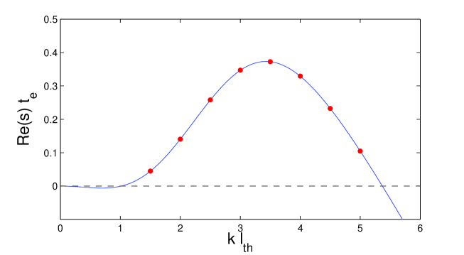
Figure 1: Linear growth rates of the ballistic transport instability as a function of wavenumber $k$, when $\tau_{0}=0.5$ and $\mu=0.025$. The solid line represents the analytical theory (see Paper 1). The points are the growth rates computed from eight numerical simulations.

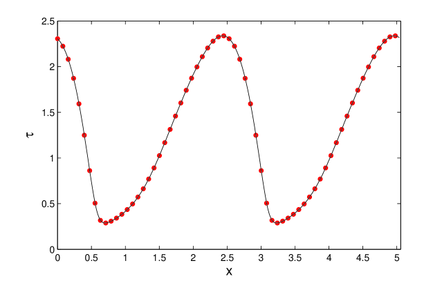
Figure 2: Two periods of a nonlinear wavetrain calculated by the numerical simulation and the direct methods of Paper 2. The solid curve represents the latter, and the dots the former after being evolved forward by the code for 10 periods, i.e. $t=2029$. Parameters are $\tau=1.3$, $\mu=0.025$, and the wavenumber is $k=2.4849$.

2.5 Numerical tests

We present two tests that demonstrate the accuracy of our numerical tool. The first one checks that the code reproduces the linear growth rates of low-amplitude disturbances. We seed two wavelengths of an unstable mode of specified wavenumber $k$ and amplitude $\sim 10^{-6}$, and then evolve it forward until it grows by at least two orders of magnitude. We subsequently measure the growth rate and compare with the analytic dispersion relation of the linear modes (cf. Eq. (49) in Paper 1). Our results are plotted in Fig. 1. The agreement is good, with the relative errors below 1%.

The second numerical test assesses the code’s handling of nonlinear waves. For initial conditions we employ two wavelengths of a nonlinear solution to (1) computed using the methods of Paper 2 and thence propagate the wavetrain for exactly 10 periods. In Fig. 2 we show the result of a typical test; the solid line represents the initial condition at $t=0$, and the dots represent the wavetrain after exactly 10 periods, $t\approx 2029$. The excellent agreement in the shape and location of the two waves confirm that the wave profiles and speed are accurately reproduced by the code. Again, the relative error falls below 1%.

3 C-ring simulations: low-amplitude wavetrains

In this section we explore the low-$\tau$ regime relevant to the C-ring. As discussed in Paper 2, the BTI in this setting forms steady wavetrains of small amplitude, and we find that it is the emergence and competition between these structures that characterises the nonlinear evolution of the instability.

3.1 Periodic boundaries: free wavetrains

Our initial run employs periodic boundary conditions, and sets $\tau_{0}=0.175$ with a constant $\mu=0.025$. The value for $\tau$ is slightly larger than observed but presents results that are easier to interpret. We restrict the size of the domain $L$ to twenty times $l_{\text{th}}$. As argued in Paper 2, structures in Saturn’s C-ring indicate that $l_{\text{th}}\sim 500$ km, and so $20l_{\text{th}}$ approximately encompasses the extent of wave activity in the C-ring. It is also near the local model’s limit of applicability. The initial condition is small-amplitude white noise $\sim 10^{-5}$, and the simulation is run for 1000 erosion times.

Results are plotted in Figs 3 and 4. The first figure shows the evolution of the perturbation amplitude, which we meaure by $\text{max}[\tau-\tau_{0}]$. The second figure presents six snapshots of $\tau$ at different (unequally spaced) times. The early stages of the evolution witness the independent and exponential growth of competing linear BTI modes, with e-folding times $\sim 100$ (see Fig. 1 in Paper 2). By $t=150$ the system is dominated by the fastest growing mode, associated with the wavenumber $k=2.827$ (thus nine wavelengths fit into the domain). This mode, low in amplitude and still roughly sinusoidal in shape, can be observed in the first panel of Fig. 4.

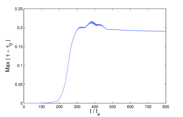
Figure 3: Time evolution of the disturbance amplitude as a result of the BTI’s growth (see Section 3.1). The initial condition is small-amplitude white noise; physical parameters are $\tau_{0}=0.175$ and $\mu=0.025$, while numerical parameters are $L=20l_{\text{th}}$ and $N=512$.

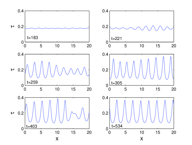
Figure 4: Six snapshots of the evolution of $\tau$ due to the BTI, as described in Section 3.1. In all panels the wave crests are moving to the left (inward), though the longer waves in panel 6 do so extremely slowly.

The exponential growth ceases after some 250 erosion times, as the system approaches the exact steady nonlinear wavetrain solution associated with $k=2.827$. However, as panels 2-5 in Fig. 4 indicate, the waveform exhibits significant modulational perturbations, conspicuous as early as $t=220$. These correspond to the action of a secondary instability upon the $k=2.827$ wavetrain; as shown in Section 4 in Paper 2, the wavetrain is too short to be stable for these parameters. Not long after $t=400$ the secondary instability destroys the $k=2.827$ solution, which is superseded by the longer (and linearly stable) $k=2.513$ solution (panel 6). Over the course of the next few hundred erosion times, the amplitude slowly relaxes to the value predicted by Paper 2 (roughly 0.19, see Fig. 3).

This general pattern of behaviour is reproduced by all parameter choices we have tried, and is thus not limited to the small $\tau_{0}$ regime. At first the fastest growing mode dominates the evolution and the system approaches a wavetrain of the same wavenumber; but because this wavetrain is always unstable, the system eventually migrates away and seeks a linearly stable longer-wavelength solution. Depending on the size of the domain (and hence the number of available modes), this process can take one step (as above) or several steps. This is in contrast to analogous behaviour in the viscous overstability, where the wavelength selection procedure is more involved — mainly because the fastest growing wavelength and the first stable wavelength are much further apart (Latter & Ogilvie 2009, 2010). Similar behaviour also occurs when the initial condition is a long unstable nonlinear wavetrain (with $k<2.225$). These solutions break up relatively quickly and the system settles on a stable shorter-wavelength wavetrain.

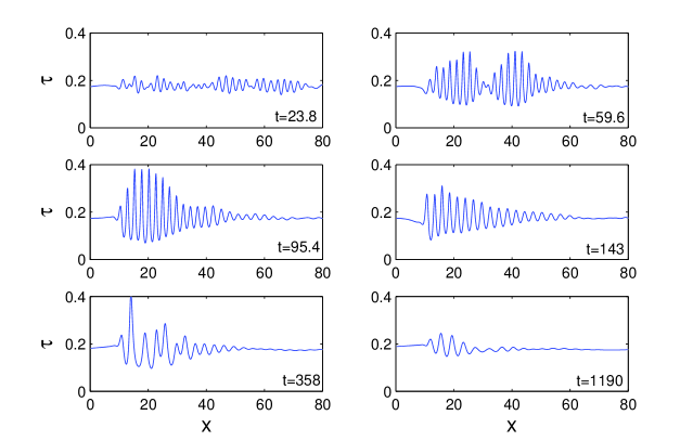
Figure 5: Six snapshots of a run with buffered domains. Here $L=100$ and $l_{B}=10$. Main parameters are $\tau=0.175$ and $\mu_{0}=0.025$. Waves crests propagate inward in panels 1 and 2, and mainly outward in panels 3-6. The group velocity of the disturbances, however, always points inward.

3.2 Buffered boundaries

The periodic box simulations of Section 3.1 indicate that the BTI, when present, always takes the system to a uniform and stable travelling wavetrain. This outcome, however, could be viewed as an artefact of the boundary conditions and the limited extent of the box. When periodic boundary conditions are imposed, the system ‘senses’ the translational symmetry of the domain after a sufficiently long time and is thus attracted to the steady wavetrain solutions admitted by this symmetry. But in the real rings there is no radial periodicity or global translational symmetry. As a consequence, steady uniform wavetrains are not exact nonlinear solutions globally – though they are approximate solutions locally – and hence cannot function as global attractors. The real rings will certainly exhibit nonlinear wavetrains, and the secondary instabilities that assail them, yet the larger-scale dynamics may be rather different to that shown in Section 3.1. They may instead exhibit a competition between different wavetrain solutions, propagating towards or away from each other, partly controlled by underlying gradients and inhomogeneities in the background state.

This subsection probes some of this behaviour by breaking the translational symmetry of the box. Buffer regions are imposed across both boundaries, as decribed in Section 2.3. These eliminate the attracting stable wavetrain solutions from the phase space, thus permitting a more realistic and interesting set of dynamics to develop. Our main simulation takes a mean optical depth $\tau_{0}=0.175$, a large domain $L=100$, and buffers of size $l_{B}=10$. White noise of moderate amplitude $(\sim 0.01)$ is seeded in order to speed up the evolution. The resulting evolution is summarised in Fig. 5, where we show six snapshots.

The fastest growing modes dominate the initial stages of the evolution, and after growing to appreciable amplitudes they undergo complicated interactions involving beating patterns and the formation of localised wave packets (panels 1 and 2). The group velocity of these waves $c_{g}$ is negative and relatively large $\sim-0.5$ (see Fig. 3b in Paper 2). As a result, disturbances propagate to the inner boundary on relatively short timescales where, over the course of the simulation, they mostly disappear into the buffer zone. Ultimately the system settles into a quasi-steady state characterised by low-amplitude long-wavelength waves with positive phase speeds (panel 6). These waves emerge from a ‘source’ at the inner buffer and decay to zero as their crests propagate outwards. Though their phase speed $c_{p}$ is positive, the group velocity of these long waves remains negative (Fig. 3b, Paper 2); thus disturbances at larger $x$ cannot be replenished by activity in the inner regions. Activity persists in the inner regions, on the other hand, as ‘residue’ of the nonlinear behaviour in the first 100 erosion times.

The key feature controlling these dynamics is the ‘convective’, as opposed to ‘absolute’, nature of the BTI: unstable waves do not grow in place, but travel as they grow. A disturbance will reach large amplitudes but it may leave the region of interest before it does so, especially if the growth time (the inverse of the linear growth rate $s$) is longer or similar to $L/c_{g}$, i.e. the time it takes for information to traverse the domain. As a consequence, any given ring region may eventually return to its undisturbed state. (This scenario is in marked contrast to the unbuffered periodic simulation of Section 3.1, where travelling disturbances are never lost and indeed can positively reinforce themselves.) In the buffered simulation described by Fig. 5, $1/s\sim L/c_{g}$. As a result, the disturbances just attain sufficiently large amplitudes for nonlinear interactions to ensue, and hence for activity to be sustained, though at a fairly low level.

To further test this idea, we conducted additional simulations, one with $L$ reduced by half and another with smaller amplitude initial conditions $\sim 10^{-4}$. In both simulations, growing disturbances propagate out of the active zone before they achieve significant amplitudes, and eventually the ring returns to a near homogeneous state. We also ran a simulation illustrating the opposite extreme, in which the growth time $1/s$ is much smaller than $L/c_{p}$; we set $\tau$ to 0.5 and hence $s\sim 0.4$, an order of magnitude larger than in Fig. 5. The results of this last simulation are summarised in Fig. 6, which displays three snapshots at different times. Note that here $l_{B}=20$. Initially, the fastest-growing modes dominate the active region, leading to the emergence of wave packets travelling inwards. After an internal wavelength selection process (panel 2), the system settles on a long wavetrain with $k\approx 1.96$ (panel 3) and positive $c_{p}$. The key point is that, because of the large growth rates, disturbances attain large amplitudes before hitting the inner buffer, allowing the nonlinear dynamics sufficient time to develop and sustain activity throughout the entire central region.

We expect some of this behaviour to characterise the low-amplitude undulations in the C-ring, which occur in a regime near marginal stability and in a relatively small domain ($\sim 20l_{\text{th}}$). If left to evolve independently for sufficient time, it is possible that the present undulations may simply propagate out of the region and disappear at the inner edge of the C-ring. Alternatively, larger amplitude disturbances may have already left the system, leaving behind the low-amplitude waves we see today; these may then correspond to the undulations in panel 6 in Fig. 5. A third, more likely scenario, is that the C-ring suffers a a continual supply of noise which reseeds the BTI and replenishes the undulations. A complication in all three hypotheses is that the waves travel through an environment punctuated by disruptive features, such as plateaus, ringlets, and gaps, as well as possible large-scale gradients in ring properties (Figs 13.17 and 13.21 in Colwell et al. 2009, Hedman et al. 2013, Fillachione et al. 2013). Finally, we note the longer wavelengths produced by our simulations ($k\approx 1.5$), which suggest an estimate for $l_{\text{th}}$ closer to 300 km, shorter than estimates based on linear stability (see Section 4 in paper 2).

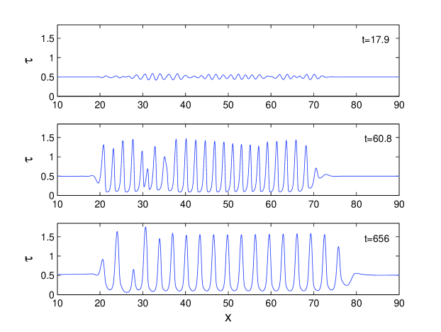
Figure 6: Three snapshots of a run with buffered boundaries. Here $L=100$ and $l_{B}=20$. The mean optical depth is $\tau=0.5$, and $\mu_{0}=0.025$. Waves characterise the simulation, the crests propagating inward in the first two panels and outward in the last.

4 Inner B-ring simulations: wavetrain pulses

This section presents simulations that approximate conditions in the inner B-ring. As discussed in Paper 2, this region is of special interest because it can exhibit bistability, whereby the system falls into a homogeneous ‘flat’ state, or a small set of large-amplitude ‘wave’ states. It is then possible that the ring radially breaks up into adjoining flat and wave zones, with the boundaries between the regions undergoing their own dynamics. We focus on this scenario here and show that this is indeed possible.

Our fiducial B-ring run takes parameters $\tau_{0}=1.3$ and $\mu=0.025$, which admit the linearly stable homogeneous state $\tau=\tau_{0}$. As explored in Section 3.3 in Paper 2, these parameters also support a number of travelling nonlinear wavetrains. Our initial condition comprises a portion of a wavetrain, possessing $k=2.5$, inserted between $x=10$ and $x=30$. The remainder of the domain is set to $\tau=\tau_{0}$. The two ends of the wavetrain are abruptly smoothed to the homogeneous value over a few grid cells. The initial condition is hence a ‘wave packet’ or ‘wave zone’. The size of the box is $L=50$, and we reinstate the periodic boundary conditions (without buffers).

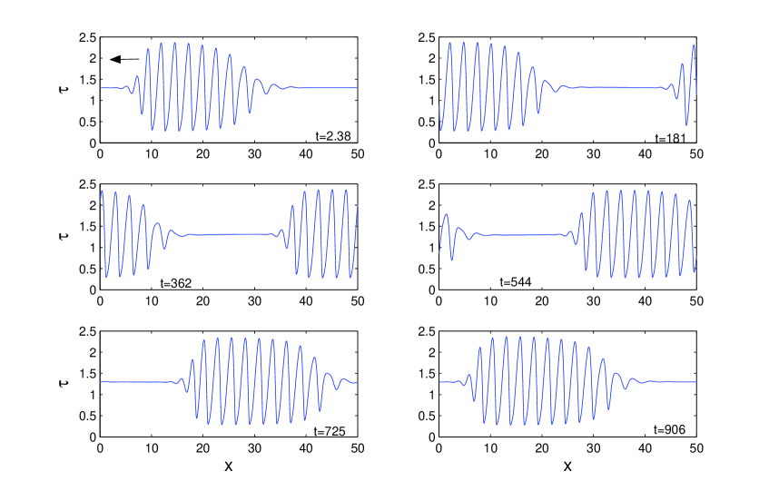
Figure 7: Six snapshots showing the evolution of BTI wavepacket propagating through a bistable ring. The background is described by $\tau_{0}=1.3$, $\mu=0.025$, and the numerical parameters are $L=50l_{\text{th}}$, and $N=1024$. The wave packet and its constituent waves travel to the left at different speeds. In addition, the front of the packet travels faster than the rear of the packet, leading to its spreading. An arrow is included indicating the direction of propagation.

Six snapshots of the evolution are displayed in Figure 7 at equally spaced times. We find that within the packet the individual peaks of the wavetrain travel to the left with the phase speed $c_{p}\approx-0.014$ predicted by the calculations of Paper 2. Moreover, the wavepacket as a whole travels to the left with the faster group speed $c_{g}=d\omega/dk\approx-0.058$, associated with $k=2.5$. As the wave packet propagates it also spreads, which is clear from the first and last snapshots in Fig. 7: after one traversal of the domain the rear of the packet has lagged behind the packet’s leading front. This is because the packet’s component wavelengths at its front are shorter than at its rear. Consequently $c_{g}$ decreases throughout the packet. The rear moves slower, and the structure as a whole spreads.

The wave packets, understood as homoclinic orbits in phase space, share a number of features with localised oscillatory states in a variety of driven and/or bistable systems. Notable examples include the complex Ginzburg Landau equation (Aranson & Kramer 2002, Burke et al. 2008), plane Couette flow (Schneider et al. 2010), and magnetoconvection (Buckley & Bushby 2013). However, because $c_{g}$ varies throughout the packet and $\neq c_{p}$, our BTI structures resist the usual techniques of dynamical systems (e.g. Burke & Knobloch 2007). In particular, as the packet spreads in time, there are no distinct states comprising the classical ‘snakes and ladders’ pattern in the phase space. Instead, over time, the system progresses through a continuum of such states.

Qualitatively, these results agree relatively well with Cassini observations which reveal that the inner B-ring radially splits into two ‘flat’ zones, where the photometric $\tau$ is constant, circumscribed by three ‘wave’ zones, exhibiting nonlinear wavetrains of wavelength $\sim 100$ km and amplitude $\sim 1$ in $\tau$ (Figs 13.11 and 13.13 in Colwell et al. 2009). We hence identify the flat zones with the inactive homogeneous state $\tau=\tau_{0}$ and the wave zones with travelling (and spreading) wave packets. Our results then suggest that the two flat zones are shrinking and will ‘evaporate’ entirely in $\sim 100t_{e}$. Of course, the Janus/Epimetheus 2:1 inner Lindblad resonance situated between the two flat zones does complicate things, but the overall agreement encourages us to view the inner B-ring as controlled by the BTI’s bistable dynamics.

A number of intriguing discrepancies remain, however. As discussed in Paper 2, the troughs of the theoretical wave profiles (measured in dynamical $\tau$) are lower than those exhibited by the observed waves (measured in photometric $\tau$). The disagreement could disappear once the differences between photometric and dynamical optical depth are corrected for, but this is not yet certain. Another, potentially related, problem issues from the discrepancy between the observed mean photometric optical depth in the flat and wave zones (Colwell et al. 2009). If this indeed corresponds to significant differences in the surface density (hence dynamical $\tau$), then our picture of the B-ring dynamics will need to be modified. A final point is that it can be difficult to seed a travelling wave packet in our theoretical simulations; an arbitrary localised large-amplitude perturbation is usually insufficient. A wavelike or very large-amplitude disturbance does better. Sources for appropriate disturbances may be present in the Janus/Epimetheus resonace, the inner B-ring edge, or the transition to the high-$\tau$ regions in the mid B-ring, but again this is uncertain.

5 Simulations of the inner B-ring edge

We finish our numerical study with a handful of exploratory simulations of a sharp ring edge spreading under the action of viscosity and ballistic transport. So far we have reproduced the dynamics of the BTI mostly in isolation of strong inhomogeneities. In this section we see how it fares in the presence of a dramatic variation in $\tau$.

We employ an initial condition representing an isolated wide ringlet possessing extremely sharp edges, as described by Eq. (10) in Section 2.4. In order to simplify the numerical results, we take the optical depth of the ringlet to be sufficiently high so that no wavetrains are possible, thus $\tau=1.5$. Similarly, in the surrounding medium we take $\tau$ to be sufficiently low so that the BTI is suppressed. We then focus exclusively on the dynamics of the inner edge of the ringlet, and treat it as an approximation to the inner edge of the B-ring. The viscosity, represented by the parameter $\mu$, is expected to vary between the low and high $\tau$ regions in our setup (Araki & Tremaine 1986, Wisdom & Tremaine 1988, Daisaka et al. 2001). However, for our main runs we let it remain a constant; additional simulations in which $\mu$ is a power law in $\tau$ do not exhibit qualitatively different results. In keeping with previous work, we associate $t_{e}$ with the erosion time of the high-$\tau$ region.

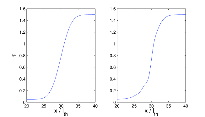
Figure 8: The $\tau$ profile of two ring edges at $t=43.56$. The initial condition in both cases is a step function, but the left panel shows an edge evolved under the action of viscous diffusion alone, while the right shows spreading under the action of both ballistic and viscous transport. In both simulations $\mu=0.065$ and is constant.

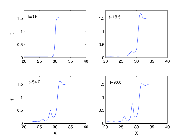
Figure 9: Four snapshots showing the spreading of a sharp edge with $\mu=0.025$ and constant.

Our first runs take a relatively large $\mu$, equal to $0.65$. Consequently, the BTI will not work for any $\tau$ (see Fig. 2 in Paper 2). This setup permits us to study the influence of ballistic transport on ring spreading in isolation of the instability itself. For comparison, we also perform a simulation with ballistic transport completely de-activated, leaving the edge to spread via viscous diffusion alone. Figure 8 shows two snapshots taken at the same time from these two simulations. While the purely viscous simulation exhibits the self-similar tanh solution of the classical diffusion equation, the BT simulation reveals a more complex structure. A characteristic ‘ramp’ profile develops at the foot of the edge, exhibiting a shallower gradient than the tanh profile. Meanwhile the edge itself remains sharper in comparison to pure viscous spreading.

These results should be compared with the more viscous runs of D92; see their Figs 4 and 5 (for which $Y=3\times 10^{4}$ and $Y=1\times 10^{5}$ respectively). The most viscous D92 run (their Fig. 4) resembles our Fig. 8a, presumably because BT is sub-dominant. The corresponding $\mu$ is difficult to calculate because of uncertainty in the value of $l_{\text{th}}$, and also because the D92 viscosity is not constant. Its mean value we estimate to be $\gtrsim 0.1$, consistent with our results. D92’s intermediate run (their Fig. 5), yields an edge profile similar to our Fig. 8b, and indeed possesses a comparable mean $\mu$ (roughly 0.05). The main difference is the absence of a ‘hump’ on the high-$\tau$ side of the edge. In fact, our $\mu=0.065$ simulation does exhibit a hump at earlier times, but it has diffused away by $t=10$. Perhaps this small discrepancy is due to our adoption of the simpler absorption probability function $P$ (see discussion in Papers 1 and 2). Overall, however, we confirm the findings of D92 that ballistic transport can maintain the sharpness of a spreading edge, and concurrently develop a ‘ramp-like’ feature at its foot.

The ramp in Figure 8b possesses values of $\tau$ which place it in the favourable range for BTI (see Fig. 2 in Paper 2). However, our choice of $\mu$ prevents instability. To test whether the ramp region can indeed support instability, we reduce $\mu$ to a value of $0.025$ and redo the numerical calculation. In Fig. 9 we present six snapshots of the ensuing evolution. Indeed, as early as $t=18$ a growing undulation appears at the foot of the edge (panel 2). As the ramp expands and generates greater $\tau$, more and more of the region becomes unstable leading to the emergence of further growing modes. Throughout this phase, the edge itself remains relatively sharp and now exhibits the hump on the high $\tau$ side. At later times the ensuing wavetrain amplitudes reach levels $\sim 1$, and the waves propagate slowly inwards.

Similar growing modes are not observed in D92’s low viscosity run (see their Fig. 6, which has $Y=3\times 10^{5}$), even though it possesses a comparable mean $\mu$ ($\sim 0.01$). The most prominent feature in the D92 run, in fact, is the high $\tau$ wavetrain, which we have suppressed by our choice of $\tau$ in the optically thick ringlet. Note, however, that the D92 simulation is only run till $t=41$, and so it is possible that appreciable BTI waves would have emerged at later times. Moreover, more recent runs by the same group witness growing ‘humps’ in the ramp for certain parameter choices (Durisen, private communication). We conclude that ramp stability is sensitive to input physics and its parameters.

Observations of the inner B-ring edge do not indicate the existence of BTI; the ramp, in fact, exhibits a remarkably unblemished linear profile (Fig. 13.21, Colwell et al. 2009). It is also unlikely that the C-ring plateaus are related to the emergence of these BTI undulations. The morphologies of the two are dissimilar and there is no positive gradient in background $\tau$ where plateaus exist, in contrast to our simulations; the observations indicate that ramps and plateaus appear separately. We hence conclude that the BTI is suppressed at the inner B-ring edge, though the responsible physical process is unclear, and obviously absent from our model. It is possible that our choice of distribution function $f$, or the parameters that appear in it, may unrealistically boost instability in this region. But more work, with further refinements, is needed before this can be verified.

Finally, we speculate that, because the ramp increases in size as the edge spreads, the ramp width could be used as a diagnostic for the ring spreading time, possibly even allowing researchers to construct past morphologies and probe ring formation scenarios. For example, the observed ramp is $\approx 1000$ km, or possibly $\approx 10l_{\text{th}}$; our simulations indicate that such a structure would take $\approx 100t_{e}$ to form, if the edge was initially very sharp.

6 Conclusion

In this paper we have developed a reliable and efficient numerical tool with which to simulate the ballistic transport process in planetary rings. We have subsequently reproduced the nonlinear evolution of the BTI in models of both the C-ring and B-ring, in addition to the spreading of a ring edge.

Both our B-ring and C-ring simulations validate the predictions of Paper 2’s semi-analytic theory. C-ring simulations saturate by forming stable low-amplitude wavetrains within a narrow range of preferred wavelengths. But because of the translational symmetry of our local model this outcome is not a global solution to the real, radially structured, C-ring. In order to eliminate some of the unrealistic effects of the translational symmetry, additional simulations were conducted with buffered boundaries. Near marginality, as in the C-ring, BTI modes possesses low growth rates and yet retain relatively large group velocities and, as a consequence, the BTI’s ‘convective’ character becomes important. Our buffered simulations show that unstable disturbances can propagate out of the region of interest before their nonlinear dynamics develop and sustain appreciable amplitudes. Unless continually fed new perturbations, the BTI may saturate at a very low level of activity. It is possible that the C-ring has fallen into such a state. However, C-ring undulations compete with other features, such as plateaus, ringlets, and gaps that may interfere with their evolution, or alternatively help seed fresh BTI modes. Undoubtedly the dynamics are complicated in this region and more irregular than predicted by the local shearing sheet with pure periodic boundary conditions.

Our simulations of the inner B-ring show that it is possible that the system splits into stable wave zones and stable homogeneous zones, in agreement with Cassini data. Moreover, the wave zones propagate through the homogeneous regions as independent wave packets while simultaneously spreading. Consequently, both the observed larger and smaller flat spots may evaporate in a time $\sim 100t_{e}\sim 10^{7}-10^{9}$ yr. However, as discussed in Paper 2, the morphologies of the theoretical and observed B-ring waves exhibit troubling discrepancies. The troughs of the former are too deep, while the mean $\tau$ in the former varies between flat and wavy zones. The disagreement could issue from the simple fact that the theoretical and observational profiles are measured in dynamical and photometric optical depths, respectively. But further work is needed to establish this directly.

Finally, we conducted exploratory simulations of the inner B-ring edge. We find that ballistic transport does not arrest the viscous spreading of the edge, but resculpts it as it spreads. In particular, ballistic transport forms a ramp-like feature at its base, while maintaining the sharpness of the edge — in agreement with previous simulations. We also find, in low viscosity runs, that the ramp structure is susceptible to BTI. But as the observed ramp does not exhibit wave (or any other) features, we conclude that the BTI is suppressed in this region by physics not captured in our fiducial simulations.

In the future we hope to refine our physical model and conduct more detailed simulations, especially of spreading edges. There are two obvious improvements: the inclusion of a $\tau$-dependent viscosity, and an absorption probability $P$ that depends on $\tau$ at both the emitting and absorbing radius. Preliminary simulations indicate little qualitative change when $\mu$ is an increasing function of $\tau$. On the other hand, a better $P$ model may alter our results more significantly, not only for the C-ring dynamics but for conditions at the inner B-ring edge. Indeed, it may aid in the suppresion of the BTI in the ramp region. Unfortunately the more realistic $P$ precludes use of the convolution theorem and its many computational benefits. An intermediate model, however, need only incorporate the first few terms in an expansion of $P$ (i.e. the first few ejecta ring-plane crossings), and the convolution theorem could then be applied to each term.

Simulations with the improved model may better reproduce, and help explain, the observed morphologies of spreading edges. They may also constrain the spreading time of the inner A-ring and B-ring by examining the widths of their ramp regions. Other targets for research include the C-ring plateaus. BTI does not generate these features and, being too narrow, nor does it emerge within them. But ballistic transport may sculpt their structure, and in particular sharpen their front and rear edges. Future numerical work here would complement previous investigations which used a descendent of the D92 code (Estrada & Durisen 2010). It could also explore a possible connection between the C-ring plateaus and similarly sized narrow rings, such as the $\epsilon$ ring in the Uranian system.

References

- (1) Aranson, I.O., Kramer, L., 2002. RvMP, 74, 99.
- (2) Buckley M. C., Bushby P. J., 2013. PRE, 87, 023019.
- (3) Burke, J., Knobloch, E., 2007. Chaos, 17, 037102.
- (4) Burke, J., Yochelis, A., Knobloch, E., 2008. SIAM J. Appl. Dyn. Syst. 7, 651.
- (5) Canuto, C., Hussaini, M. Y., Quarteroni, A., Zang, T. A., 2006. Spectral Methods: Fundamentals in Single Domains, Springer, Berlin Germany.
- (6) Charnoz, S., Dones, L., Esposito, L.W., Estrada, P.R., Hedman, M.M., 2009. In: Dougherty, M. K., Esposito, L. W., Krimigis, S. M. (eds.), Saturn from Cassini-Huygens, Springer, Dordrecht Netherlands, p537.
- (7) Colwell, J. E., Nicholson, P. D., Tiscareno M. S., Murray, C. D., French, R. G., Marouf, E. A., 2009. In: Dougherty, M. K., Esposito, L. W., Krimigis, S. M. (eds.), Saturn from Cassini-Huygens, Springer, Dordrecht Netherlands, p375.
- (8) Cuzzi, J. N., Durisen, R. H., 1990. Icarus, 84, 467. (CD90)
- (9) Daisaka, H., Tanaka, H., Ida, S., 2001. Icarus, 154, 296.
- (10) Durisen, R. H., 1984. In: Greenberg, R., Brahic, A., (Eds), Planetary Rings, University if Arizona Press, Tucson, p416.
- (11) Durisen, R. H., 1995. Icarus, 115, 66. (D95)
- (12) Durisen, R. H., Cramer, N. L., Murphy, B. W., Cuzzi, J. N., Mullikin, T. L., Cederbloom, S. E., 1989. Icarus, 80, 136. (D89)
- (13) Durisen, R. H., Bode, P. W., Cuzzi, J. N., Cederbloom, S. E., Murphy, B. W., 1992. Icarus, 100, 364. (D92)
- (14) Estrada, P., Durisen, R., 2010. 41st Lunar and Planetary Science Conference Abstracts, p2686.
- (15) Filacchione, G. and 13 co-authors, 2013. ApJ, 766, 76.
- (16) Hedman, M. M., Nicholson, P. D., Cuzzi, J. N., Clark, R. N., Filacchione, G., Capaccioni, F., Ciarniello, M., 2013. Icarus, 223, 105.
- (17) Ip, W.-H, 1984. Icarus, 60, 547.
- (18) Latter, H. N., Ogilvie, G. I., 2009. Icarus, 202, 565.
- (19) Latter, H. N., Ogilvie, G. I., 2010. Icarus, 210, 318.
- (20) Latter, H. N., Ogilvie, G. I., Chupeau, M., 2012. MNRAS, 427, 2336. (Paper 1.)
- (21) Latter, H. N., Ogilvie, G. I., Chupeau, M., 2013. MNRAS, submitted. (Paper 2.)
- (22) Lissauer, J. J., 1984. Icarus, 57, 63.
- (23) Schneider T., Gibson J., Burke J., 2010. PRL. 104, 104501.