Hierarchical analysis-suitable T-splines: Formulation, Bézier extraction, and application as an adaptive basis for isogeometric analysis

Abstract

In this paper hierarchical analysis-suitable T-splines (HASTS) are developed. The resulting spaces are a superset of both analysis-suitable T-splines and hierarchical B-splines. The additional flexibility provided by the hierarchy of T-spline spaces results in simple, highly localized refinement algorithms which can be utilized in a design or analysis context. A detailed theoretical formulation is presented including a proof of local linear independence for analysis-suitable T-splines, a requisite theoretical ingredient for HASTS. Bézier extraction is extended to HASTS simplifying the implementation of HASTS in existing finite element codes. The behavior of a simple HASTS refinement algorithm is compared to the local refinement algorithm for analysis-suitable T-splines demonstrating the superior efficiency and locality of the HASTS algorithm. Finally, HASTS are utilized as a basis for adaptive isogeometric analysis.

1 Introduction

In this work, a hierarchical extension of analysis-suitable T-splines is developed and utilized in the context of isogeometric design and analysis. We call this new spline description hierarchical analysis-suitable T-splines (HASTS). The class of HASTS is a strict superset of both analysis-suitable T-splines [1, 2, 3, 4, 5] and hierarchical B-splines [6, 7, 8, 9, 10, 11].

T-splines, introduced in the CAD community [12], are a generalization of non-uniform rational B-splines (NURBS) which address fundamental limitations in NURBS-based design. For example, a T-spline can model a complicated design as a single, watertight geometry and are also locally refinable [13, 2]. Since their advent they have emerged as an important technology across multiple disciplines and can be found in several major commercial CAD products [14, 15].

Isogeometric analysis was introduced in [16] and described in detail in [17]. The isogeometric paradigm is simple: use the smooth spline basis that defines the geometry as the basis for analysis. As a result, exact geometry is introduced into the analysis, the smooth basis can be leveraged by the analysis [18, 19, 20], and new innovative approaches to model design [21, 22], analysis [7, 23, 24, 25], optimization [26], and adaptivity [27, 28, 9, 9] are made possible. The use of T-splines as a basis for isogeometric analysis (IGA) has gained widespread attention across a number of application areas [27, 29, 2, 30, 31, 32, 25, 7, 23, 33, 34, 35, 36, 37, 38]. Particular focus has been placed on the use of T-spline local refinement in an analysis context [2, 32, 31, 30].

In the context of CAD, where a designer interacts directly with the geometry, T-spline local refinement is most useful if confined to a single level. In other words, all local refinement is done on one control mesh and all control points have similar influence on the shape of the surface. In this way, the geometric behavior of the surface is easily controlled through the manipulation of control points before and after refinement. In the context of analysis, however, where not all control points need to have a geometric interpretation, the single level restriction can be relaxed. This hierarchical point of view has important advantages:

1. Hierarchical local refinement remains completely local. Single level T-spline local refinement always entails a degree of nonlocal control point propagation [2].

2. Hierarchical local coarsening is achieved by simply removing higher levels of refinement where needed [9]. Local coarsening operations for single level T-spline descriptions are possible but their algorithmic complexity remains uncertain [13].

3. Hierarchical refinement and coarsening operations use a fixed control mesh which simplifies algorithmic developments, especially for parallel computations. Single level local refinement requires expensive mesh manipulation and modification operations.

4. Hierarchies of finite-dimensional subspaces are the natural setting for many optimized iterative solvers and preconditioning techniques for large-scale linear systems.

Initial investigations employing hierarchical B-spline refinement in the context of IGA have demonstrated the promise of the hierarchical approach [39, 7, 40, 41, 42].

HASTS inherit the design strengths of T-splines without the single level restriction. In this way, a complex T-spline design can be encapsulated in the first level of the hierarchy while higher levels can be leveraged to develop adaptive multiresolution schemes which are smooth, highly localized, geometrically exact, and appropriate for the analysis task at hand. We feel that this provides the appropriate mathematical foundation for the development of integrated isogeometric design and analysis methodologies for demanding applications in science and engineering. Note that, in this paper, we restrict our theoretical developments to HASTS defined over four-sided domains. However, extending HASTS to domains of arbitrary topological genus should be straightforward in the context of the recently introduced spline forest [9].

We note that in addition to T-splines, hierarchical B-splines, and NURBS a number of alternative spline technologies have been proposed as a basis for IGA with varying strengths and weaknesses. Truncated hierarchical B-splines (THB-splines) [11, 43, 44, 45] are a modification of hierarchical B-splines [6, 8, 40] which possess a partition of unity and enhanced numerical conditioning. B-spline forests [9] are a generalization of hierarchical B-splines to surfaces and volumes of arbitrary topological genus. Polynomial splines over hierarchical T-meshes (PHT-splines) [46, 47, 48, 49], modified T-splines [50], and locally refined splines (LR-splines) [51, 52] are closely related to T-splines with varying levels of smoothness and approaches to local refinement. Generalized B-splines [53, 54] and T-splines [55] enhance a piecewise polynomial spline basis by including non-polynomial functions, typically trigonometric or hyperbolic functions. Generalized splines permit the exact representation of conic sections without resorting to rational functions. Generalized splines can also be used to represent solution features with known non-polynomial characteristics exactly in certain circumstances.

1.1 Structure and content of the paper

In Section 2 the T-mesh is described and appropriate notational conventions are introduced. Analysis-suitable T-splines are then described in Section 3. The local linear independence of analysis-suitable T-splines is established in Section 4. Hierarchical analysis-suitable T-splines are then defined in Section 5. In preparation for their use in design and analysis a Bézier extraction framework is introduced in Section 6. HASTS are then utilized as a basis for isogeometric analysis in Section 7. In  Section 8 we draw conclusions. We note that the paper has been written so the proof of local linear independence in Section 4 is self-contained and can be skipped if the reader is not interested in the detailed theory of analysis-suitable T-splines.

2 The T-mesh

The T-mesh is used to define the topological structure of the associated T-spline space. In other words, the T-mesh defines the basis functions and their relationship to one another. We closely follow the notational conventions introduced in [5, 4, 3].

A T-mesh $\mathsf{T}$ in two dimensions is a rectangular partition of $\hat{\vphantom{\rule{1.0pt}{5.93056pt}}\smash{\hat{\Omega}}}=[1,m]\times[1,n]$ such that all vertices $V=\{i,j\}\in\mathsf{V}$ have integer coordinates. All cells $C\in\mathsf{C}$ are rectangular, non-overlapping, and open. An edge is a horizontal or vertical line segment between vertices which does not intersect any cell. The valence of a vertex $V\in\mathsf{V}$ is the number of edges coincident to that vertex. Since all cells are assumed rectangular, only valence three (i.e., T-junction) or four is allowed for all vertices $V\subset(1,m)\times(1,n)$. The sets of horizontal and vertical coordinates in the T-mesh are denoted by $h\mathsf{I}=\{1,2,\ldots,m\}$ and $v\mathsf{I}=\{1,2,\ldots,n\}$. The horizontal and vertical skeletons, $h\mathsf{S}$ and $v\mathsf{S}$, of a T-mesh are the union of all horizontal and vertical edges, respectively, and associated vertices. The entire skeleton is denoted by $\mathsf{S}=h\mathsf{S}\cup v\mathsf{S}$.

We split $\hat{\vphantom{\rule{1.0pt}{5.93056pt}}\smash{\hat{\Omega}}}$ into an active region $\mathsf{AR}$ and a frame region $\mathsf{FR}$ such that $\hat{\vphantom{\rule{1.0pt}{5.93056pt}}\smash{\hat{\Omega}}}=\mathsf{FR}\cup\mathsf{AR}$ and $\mathsf{AR}=[1+\lfloor(p+1)/2\rfloor,m-\lfloor(p+1)/2\rfloor]\times[1+\lfloor(q+1)/2\rfloor,n-\lfloor(q+1)/2\rfloor]$, and $\mathsf{FR}=\overline{\hat{\vphantom{\rule{1.0pt}{5.93056pt}}\smash{\hat{\Omega}}}\setminus\mathsf{AR}}$ where $p$ and $q$ are polynomial degrees. Note that both $\mathsf{FR}$ and $\mathsf{AR}$ are closed. Further, all T-meshes considered in this work are admissible as described in [5], a mild restriction always adopted in practice. The notation $\mathsf{T}^{1}\subseteq\mathsf{T}^{2}$ will indicate that $\mathsf{T}^{2}$ can be created by adding vertices and edges to $\mathsf{T}^{1}$. Fig. 1 shows an example T-mesh.

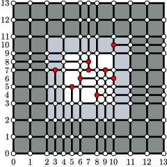
Figure 1: A bicubic T-mesh. The frame region ($\mathsf{F}$R) is dark grey and the active region ($\mathsf{AR})$ is the union of the light grey and white regions. Note that the region with zero parametric area (see Section 3.1 for a description of the parametric space of a T-spline) is the union of the dark and light grey regions.

2.1 Analysis-suitable T-meshes

Analysis-suitable T-splines (ASTS) were introduced in [1]. The analysis-suitability of a T-spline is dictated by the structure of the underlying T-mesh. We define face and edge extensions to be closed line segments that originate at T-junctions. For example, to define a horizontal face extension we trace out a horizontal line by moving in the direction of the missing edge until $\lfloor(p+1)/2\rfloor$ vertical edges or vertices are intersected. To define an edge extension we trace out a horizontal line by moving in the direction opposite the face extension until $\lceil(p-1)/2\rceil$ vertical edges or vertices are intersected. A T-junction extension includes both the face and edge extensions. Since extensions are defined as closed line segments they may intersect at their end points. An extended T-mesh, $\mathsf{T}_{ext}$, is the T-mesh formed by adding the T-junction extensions to $\mathsf{T}$. The collection of rectangular cells in $\mathsf{T}_{ext}$ is denoted by $\mathsf{C}_{ext}$. We say a T-mesh is analysis-suitable if no horizontal T-junction extension intersects a vertical T-junction extension. Face and edge extensions (along with analysis-suitability) are illustrated in Figure 2.

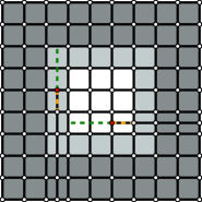
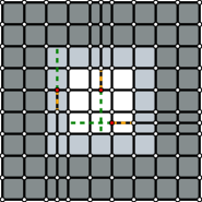
Figure 2: T-junction extension in two dimensions for a bicubic T-spline. Face extensions are shown in green and edge extensions are shown in orange. The T-mesh on the left is analysis-suitable whereas the T-mesh on the right is not due to intersecting face extensions.

2.2 Anchors

Anchors are used in the construction of T-spline blending functions. For an analysis-suitable T-mesh the anchors are located only in the active region and are defined as follows:

• if $p$ and $q$ are odd the anchors are vertices. It is written as $\{i\}\times\{j\}$ or equivalently $\{i,j\}$.

• if $p$ is even and $q$ is odd the anchors are horizontal edges. It is written as $(i_{1},i_{2})\times\{j\}$.

• if $p$ is odd and $q$ is even the anchors are vertical edges. It is written as $\{i\}\times(j_{1},j_{2})$.

• if $p$ and $q$ are even the anchors are cells. It is written as $(i_{1},i_{2})\times(j_{1},j_{2})$.

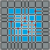
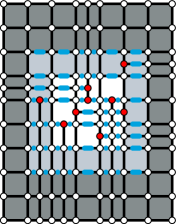
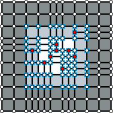
(a) $p=2,\;q=2$, anchors are the faces denoted by blue squares. (b) $p=3,\;q=2$, anchors are the vertical edges denoted by bold blue vertical lines. (c) $p=2,\;q=3$, anchors are the horizontal edges denoted by bold blue horizontal lines. (d) $p=3,\;q=3$, anchors are the vertices denoted by small blue hollow squares.

Figure 3: The set of anchors for varying values of $p$ and $q$. In this picture, the blue regions denote anchor locations. Note that no anchors reside inside the frame region (dark grey region).

The set of all anchors is denoted by $\mathsf{A}$. The set of anchors for varying values of $p$ and $q$ are shown in Figure 3.

3 Analysis-suitable T-splines

Analysis-suitable T-splines form a useful subset of T-splines. ASTS maintain the important mathematical properties of the NURBS basis while providing an efficient and highly localized refinement capability. Several important properties of ASTS have been proven:

• The blending functions are linearly independent for any choice of knots [1].

• The basis constitutes a partition of unity [5].

• Each basis function is non-negative.

• They can be generalized to arbitrary degree [4].

• An affine transformation of an analysis-suitable T-spline is obtained by applying the transformation to the control points. We refer to this as affine covariance. This implies that all “patch tests” (see [56]) are satisfied a priori.

• They obey the convex hull property.

• They can be locally refined [12, 2, 5].

• A dual basis can be constructed [3, 4].

• Optimal approximation [5].

The important properties of ASTS emanate directly from the topological properties of the underlying analysis-suitable T-mesh and resulting set of T-spline basis functions constructed from it.

3.1 T-spline basis functions, spaces, and geometry

Given a parametric domain $\hat{\Omega}=[0,1]^{2}$ we define global horizontal and vertical open knot vectors $h\mathsf{K}=\{s_{1},s_{2},\ldots,s_{m}\}$ and $v\mathsf{K}=\{t_{1},t_{2},\ldots,t_{n}\}$, respectively. In other words,

$$0=s_{1}=\ldots=s_{p+1}<s_{p+2}\leq\ldots\leq s_{m-p-1}<s_{m-p}=\ldots=s_{m}=1$$

and

$$0=t_{1}=\ldots=t_{q+1}<t_{q+2}\leq\ldots\leq t_{n-q-1}<t_{n-q}=\ldots=t_{n}=1.$$

As a result, every T-mesh vertex $V=\{i,j\}\in\hat{\vphantom{\rule{1.0pt}{5.93056pt}}\smash{\hat{\Omega}}}$ has the parametric representation $\{s_{i},t_{j}\}\in\hat{\Omega}$. For reasons that will become apparent, we refer to a cell $C\in\mathsf{C}_{ext}$ with positive parametric area as a Bézier element. The parametric domain of a Bézier element is denoted by $\hat{\Omega}^{e}$. The set of all Bézier elements in a T-mesh is denoted by $\mathsf{E}$.

For each anchor $A=a\times b\in\mathsf{A}$ we construct horizontal and vertical local index vectors $\{i_{1},\ldots,i_{p+2}\}$ and $\{j_{1},\ldots,j_{q+2}\}$ made up of increasing (but not necessarily consecutive) indices in $h\mathsf{I}$ and $v\mathsf{I}$, respectively. Note that for $p$ odd, $\{i_{(p+3)/2}\}=a$, and for $p$ even, $(i_{(p/2)+1},i_{(p/2)+2})=a$. Similar relationships hold for $q$. The procedure for determining local index vectors is shown in Fig. 4 for various polynomial degrees. To clarify this procedure we describe the anchors and associated local index vectors. In Figure 4a, ${p}=2$ and $q=2$ and thus the example anchor is the cell $(4,8)\times(3,7)$. The horizontal local index vector is $\{3,4,8,10\}$ and the vertical local index vector is $\{2,3,7,9\}.$ We observe that subset of the vertical skeleton located at index $9$ does not span the entire height of the anchor cell, hence it is not included in the horizontal local index vector; similarly since subset of the horizontal skeleton located at index $8$ does not span the entire width of the cell it not included in the vertical local index vector. In Figure 4b, ${p}=3$ and $q=2$ thus the example anchor is the vertical edge $\{9\}\times(7,j)$. The horizontal local index vector is $\{5,8,9,11,12\}$ and the vertical local index vector is $\{6,7,9,10\}.$ Similar to the prior example the subset of the vertical skeleton at index $8$ does not span the entire height of the anchor edge, hence it is not included in the horizontal local index vector. Figure 4c shows the case where ${p}=2$ and $q=3$ thus the example anchor is the horizontal edge $(4,7)\times\{8\}$. The horizontal local index vector is $\{3,4,7,8\}$ and the vertical local index vector is $\{3,4,8,9,10\}.$ In the last case, shown in Figure 4d, ${p}=3$ and $q=3$ thus the example anchor is the vertex $\{8\}\times\{8\}$. The horizontal local index vector is $\{4,5,8,9,11\}$ and the vertical local index vector is $\{3,4,8,9,10\}.$

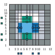
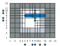
(a) $p=2,\;q=2$	(b) $p=3,\;q=2$
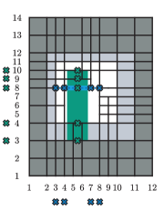
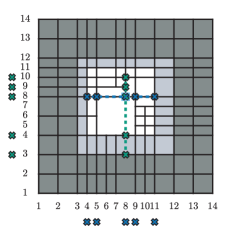
(c) $p=2,\;p=3$	(d) $p=3,\;q=3$

Figure 4: Examples for how local index vectors are constructed for T-spline basis functions of varying values of the polynomial degrees $p$ and $q$. The function anchors are marked with light blue. The horizontal line used to determine the horizontal local index vector is indicated with a dark blue dashed line. The vertical line used to calculate the vertical local index vector is marked with a green dashed line. The indices that contribute to the local index vectors are marked with $\times$.

The T-spline blending function $N_{A}^{p,q}(s,t)$ is given by

$$N_{A}^{p,q}(s,t):=N_{A}^{p}[s_{i_{1}},\ldots,s_{i_{p+2}}](s)N_{A}^{q}[t_{j_{1}},\ldots,t_{j_{q+2}}](t)\quad\forall(s,t)\in\hat{\Omega}$$ (1)

where $N_{A}^{p}[s_{i_{1}},\ldots,s_{i_{p+2}}](s)$ and $N_{A}^{q}[t_{j_{1}},\ldots,t_{j_{q+2}}](t)$ are B-spline basis functions associated with the local knot vectors $[s_{i_{1}},\ldots,s_{i_{p+2}}]\subset h\mathsf{K}$ and $[t_{j_{1}},\ldots,t_{j_{q+2}}]\subset v\mathsf{K}$.

We define $\mathsf{N}$ to be the set of all basis functions associated with a T-mesh. Given a weight $w_{A}\in\mathbb{R}^{+}$ for each $A\in\mathsf{A}$ a rational T-spline basis function $R_{A}^{p,q}:\hat{\Omega}\rightarrow\mathbb{R}$ can be written as

$$R_{A}^{p,q}(s,t) =\frac{N_{A}^{p,q}(s,t)}{\sum_{A\in\mathsf{A}}w_{A}N_{A}^{p,q}(s,t)}$$ (2)

$$=\frac{N_{A}^{p,q}(s,t)}{w(s,t)}$$ (3)

where $w(s,t):\hat{\Omega}\rightarrow\mathbb{R}$ is called a weight function. For clarity we will often suppress the dependence on the polynomial degrees $p,q$ and write the basis function as $R_{A}$. Figure 5 shows several T-spline basis functions plotted in the parametric domain $\hat{\Omega}$.

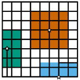
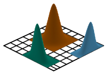
Figure 5: T-spline basis functions and supports in the parametric domain $\hat{\Omega}$ for $p=q=3$. Anchor locations are denoted by a star.

An ASTS space, denoted by $\mathcal{T}$, is the span of the blending functions in $\mathsf{N}$ constructed from an analysis-suitable T-mesh. Given vector valued control points, $\mathbf{P}_{A}\in\mathbb{R}^{n}$, $n=2$ or $3$, the geometry of a T-spline can be written as

$$\mathbf{x}(s,t)=\sum_{A\in\mathsf{A}}\mathbf{P}_{A}w_{A}R_{A}(s,t).$$ (4)

4 Local linear independence of analysis-suitable T-splines

The local linear independence of analysis-suitable T-splines is an important theoretical result in its own right and is critical for our definition of hierarchical analysis-suitable T-splines in Section 5. The (global) linear independence of analysis-suitable T-splines was first shown in [1]. Local linear independence is a stronger result than global linear independence and is the notion of linear independence enjoyed by standard $C^{0}$ finite element bases. Local linear independence implies that the finite element basis is linearly independent over every element domain. For smooth locally-refined bases this element-level notion of linear independence may be lost.

4.1 Preliminaries

Given a knot vector $\{s_{1}\leq s_{2}\leq\ldots\leq s_{m}\}$ and degree $p$ we can recursively define $n=m-p-1$ B-spline basis functions $N_{i,p}(s)$ as follows:

$$N_{i}^{0}(s)=\begin{cases}1&s_{i}\leq s<s_{i+1}\\ 0&\text{otherwise}.\end{cases}$$ (5)

$$N_{i}^{p}(s)=\frac{s-s_{i}}{s_{i+p}-s_{i}}N_{i}^{p-1}(s)+\frac{s_{i+p+1}-s}{s_{i+p+1}-s_{i+1}}N_{i+1}^{p-1}(s).$$ (6)

The de Boor algorithm [57] provides a standard method for evaluating a B-spline, although other possibilities exist [58, 59]. A B-spline basis function $N_{i}^{p}(s)$ can also be denoted by $N[s_{i},\ldots,s_{i+p+1}](s)$. Following [60], there exist dual functionals $\lambda_{j,p}=\lambda[s_{j},\ldots,s_{j+p+1}]$ such that $\lambda_{j,p}(N_{i}^{p}(s))=\delta_{j,i}$ where the Kronecker delta $\delta_{i,j}$ is zero when $i\neq j$ and one otherwise. We have the following two results:

Lemma 4.1.

Suppose $f(s)=\sum_{i=1}^{n}c_{i}N_{i}^{p}(s)$. Then $c_{j}=\lambda_{j}^{p}(f(s)).$

Lemma 4.2.

For any function $f(s)=\sum_{i=1}^{n}c_{i}N_{i}^{p}(s)$, if $f(s)=0$, $s_{k}\leq s\leq s_{k+1}$ then for $j=k-p,k-p+1,\ldots,k$ we have that $\lambda_{j}^{p}(f(s))=0.$

As shown in [4, 3] the notion of a dual basis can be extended to analysis-suitable T-splines.

Theorem 4.3.

Given an analysis-suitable T-mesh and associated basis functions $\{N_{A}^{p,q}:{A}\in\mathsf{A}_{p,q}\}$ the set of functionals $\{\lambda_{A}^{p,q}:{A}\in\mathsf{A}_{p,q}\}$ form a dual basis. Specifically, we have that

$$\lambda_{A}^{p,q}=\lambda_{A}[s_{i_{1}},\ldots,s_{i_{p+2}}]\otimes\lambda_{A}[t_{j_{1}},\ldots,t_{j_{q+2}}]$$

where $\lambda_{A}[s_{i_{1}},\ldots,s_{i_{p+2}}]$ and $\lambda_{A}[t_{j_{1}},\ldots,t_{j_{q+2}}]$ are dual basis functions corresponding to univariate B-splines [60] with local knot vectors $\{s_{i_{1}},\ldots,s_{i_{p+2}}\}$ and $\{t_{j_{1}},\ldots,t_{j_{q+2}}\}$, respectively.

4.2 Proof of local linear independence

Lemma 4.4.

Let $C\in\mathsf{C}_{ext}$ be a cell from an analysis-suitable extended T-mesh with vertices $\{i_{l},j_{b}\},$ $\{i_{r},j_{b}\},$ $\{i_{r},j_{t}\},$ and $\{i_{l},j_{t}\}$. If the basis function anchored at ${A}\in\mathsf{A}_{p,q}$ with local index vectors $\{i_{1},\ldots,i_{p+2}\}$ and $\{j_{1},\ldots,j_{q+2}\}$ is non-zero over $C$ then there must either exist an integer $k$, $1\leq k\leq p+1$, such that $i_{l}=i_{k}$ and $i_{r}=i_{k+1}$ or an integer $\ell$, $1\leq\ell\leq q+1$, such that $j_{b}=j_{\ell}$ and $j_{t}=j_{\ell+1}$.

Proof.

Suppose the lemma is false, then there exists at least one cell in $\mathsf{C}_{ext}$ that violates the condition. We denote this cell by be $C^{*}$. Since $C^{*}$ violates the condition there exists at least one corner of $C^{*}$ that lies in $\{i_{k},i_{k+1}\}\times\{j_{\ell},j_{\ell+1}\}$ where $1\leq k\leq p+1$ and $1\leq\ell\leq q+1$. Without loss of generality we may assume that $\lfloor\frac{p}{2}\rfloor+3\leq k\leq p+1$ and $\lfloor\frac{q}{2}\rfloor+3\leq\ell\leq q+1$. We have following three cases:

1. The corner is a vertex of the original T-mesh. This violates Lemma 3.2(a) in [4].

2. The corner is the result of the intersection of two perpendicular T-junction extensions. This violates the assumption that the T-mesh is analysis-suitable.

3. The corner is the result of the intersection of one T-junction extension and a T-mesh edge. Without loss of generality, we assume the edge is a horizontal edge and the T-junction extension is vertical and is associated with a T-junction $T_{1}$. As the edge cannot intersect the vertical line $i_{\lceil p/2\rceil+1}$, it must terminate in a T-junction $T_{2}$. Examining the extensions associated with $T_{1}$ and $T_{2}$ we find that they must intersect. This violates the assumption that the T-mesh is analysis-suitable.

Hence, such cell cannot exist. ∎

Theorem 4.5.

The basis for an analysis-suitable T-spline is locally linearly independent.

Proof.

Let an arbitrary Bézier element, $E\in\mathsf{E}$, from an analysis-suitable T-mesh be given. We denote the element vertices by $\{i_{l},j_{b}\},$ $\{i_{r},j_{b}\},$ $\{i_{r},j_{t}\},$ and $\{i_{l},j_{t}\}$. Let $\mathsf{A}^{e}$ be the set of anchors whose corresponding basis functions are non-zero over $\hat{\Omega}^{e}$. Assume that $f(s,t)=\sum_{A\in\mathsf{A}^{e}}c_{A}N_{A}(s,t)=0$ for all $s,t\in\hat{\Omega}^{e}$. By Lemma 4.4, since $N_{A}$ is non-zero over $E$, there exists either a $k$, $1\leq k\leq p+1$, such that $i_{l}=i_{k}$ and $i_{r}=i_{k+1}$ or an $\ell$, $1\leq\ell\leq q+1$, such that $j_{b}=j_{\ell}$ and $j_{t}=j_{\ell+1}.$ By Lemma 4.3

$$\begin{split}c_{A}&=\lambda_{A}^{p,q}(f(s,t))\\ &=\lambda_{A}[s_{i_{1}},\ldots,s_{i_{p+2}}]\otimes\lambda_{A}[t_{j_{1}},\ldots,t_{j_{q+2}}](f(s,t)).\end{split}$$

Since $f(s,t)=0$ for $s_{i_{k}}\leq s\leq s_{i_{k+1}}$ or $f(s,t)=0$ for $t_{j_{\ell}}\leq t\leq t_{j_{\ell+1}}$ we have by Lemma 4.2 that

$$\lambda_{A}[s_{i_{1}},\ldots,s_{i_{p+2}}](f(s,t))=0$$

or

$$\lambda_{A}[t_{j_{1}},\ldots,t_{j_{q+2}}](f(s,t))=0$$

which completes the proof. ∎

5 Hierarchical analysis-suitable T-splines

A hierarchical T-spline space is constructed from a finite sequence of $N$ nested ASTS spaces, $\mathcal{T}^{\alpha}\subset\mathcal{T}^{\alpha+1}$, $\alpha=1,\ldots,N-1$, and $N$ bounded open index domains, $\hat{\vphantom{\rule{1.0pt}{5.93056pt}}\smash{\hat{\Omega}}}^{N}\subseteq\hat{\vphantom{\rule{1.0pt}{5.93056pt}}\smash{\hat{\Omega}}}^{N-1}\subseteq\cdots\subseteq\hat{\vphantom{\rule{1.0pt}{5.93056pt}}\smash{\hat{\Omega}}}^{1}$, which define the nested domains for the hierarchy. Two important theoretical results for ASTS will be used in the construction of hierarchical analysis-suitable T-splines:

Theorem 5.1.

Given two analysis-suitable T-meshes with non-overlapping T-junction extensions, $\mathsf{T}^{1}$ and $\mathsf{T}^{2}$ , if $\mathsf{T}_{ext}^{1}\subseteq\mathsf{T}_{ext}^{2}$, then $\mathcal{T}^{1}\subseteq\mathcal{T}^{2}$.

Theorem 5.2.

Analysis-suitable T-splines are locally linear independent.

We note that to accommodate overlapping T-junction extensions requires a minor generalization of Theorem 5.1 which is not reproduced here to maintain clarity of exposition. For a complete description of the underlying theory we refer the interested reader to [5]. The local linear independence of ASTS is proven in Section 4.

5.1 Sequences of analysis-suitable T-meshes

We construct a sequence of $N$ analysis-suitable T-meshes such that $\mathcal{T}^{\alpha}\subseteq\mathcal{T}^{\alpha+1}$, $\alpha=1,\ldots,N-1$, as follows:

1. Create $\mathsf{T}^{\alpha+1}$ from $\mathsf{T}^{\alpha}$ by subdividing each cell in $\mathsf{E}^{\alpha}$ into four congruent cells.

2. Extend T-junctions in $\mathsf{T}^{\alpha+1}$ until it is analysis-suitable and $\mathsf{T}_{ext}^{\alpha}\subseteq\mathsf{T}_{ext}^{\alpha+1}$.

This algorithm is graphically demonstrated in Figure 6 for a particular T-mesh. For an efficient and general algorithm to produce nested analysis-suitable T-spline spaces see [2].

(a) The initial T-mesh, $\mathsf{T}^{\alpha}$.
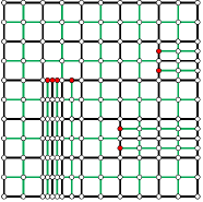
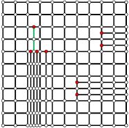
(b) Create $\mathsf{T}^{\alpha+1}$ from $\mathsf{T}^{\alpha}$ by subdividing Bézier elements.	(c) Extend T-junctions until $\mathsf{T}^{\alpha+1}$ is analysis-suitable and $\mathsf{T}^{\alpha}\subseteq\mathsf{T}^{\alpha+1}$.

Figure 6: Generating nested analsysis-suitable T-meshes. In Figures (b) and (c) the zero parametric area region is omitted for clarity.

5.2 Hierarchical T-spline spaces

The hierarchical analysis-suitable T-spline basis can be constructed recursively in a manner analogous to that used for hierarchical B-splines [8]:

1. Initialize $\mathsf{H}^{1}=\mathsf{N}^{1}.$

2. Recursively construct $\mathsf{H}^{\alpha+1}$ from $\mathsf{H}^{\alpha}$ by setting

   $$\mathsf{H}^{\alpha+1}=\mathsf{H}^{\alpha+1}_{coarse}\cup\mathsf{H}^{\alpha+1}_{fine},\alpha=1,\ldots,N-1,$$

   where

   $$\mathsf{H}^{\alpha+1}_{coarse}=\{N\in\mathsf{H}^{\alpha}:\text{supp}(N)\nsubseteq\hat{\Omega}^{\alpha+1}\},$$

   and

   $$\mathsf{H}^{\alpha+1}_{fine}=\{N\in\mathsf{N}^{\alpha+1}:\text{supp}(N)\subseteq\hat{\Omega}^{\alpha+1}\}.$$

3. Set $\mathsf{H}=\mathsf{H}^{N}.$

We denote the number of functions in $\mathsf{H}$ by $n_{f}$. We call the space spanned by the functions in $\mathsf{H}$ a hierarchical analysis-suitable T-spline space and denote it by $\mathcal{H}$. To make the ideas concrete a univariate hierarchical spline space is shown in Figure 7.

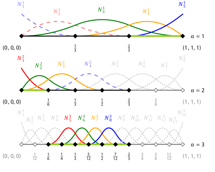
Figure 7: Basis functions for a univariate hierarchical spline space. Functions in $\mathsf{H}$ are indicated by solid colored lines. Functions dependent on higher-level functions are indicated by dashed colored lines. Functions which are not fully supported in the hierarchy of domains are indicated by grey dotted lines. Hierarchical domains are black and Bézier elements are green. Note that functions in $\mathsf{H}$ are supported entirely by Bézier elements.

The linear independence of the functions in $\mathsf{H}$ follows immediately from the definition of hierarchical T-splines and the local linear independence of ASTS (see Section 4).

Lemma 5.3.

The functions in the hierarchical basis $\mathsf{H}$ are linearly independent.

Proof.

See Lemma 2 in [8] ∎

Lemma 5.4.

Given $\mathsf{H}^{1},\ldots,\mathsf{H}^{N}$, a sequence of hierarchical analysis-suitable T-spline bases, $\operatorname{span}\mathsf{H}^{\alpha}\subseteq\operatorname{span}\mathsf{H}^{\alpha+1}$, $\alpha=1,\ldots,N-1$.

Proof.

See Lemma 3 in [8] ∎

By construction, $\mathcal{T}^{1}\subseteq\mathcal{H}$, thus the approximation properties of analysis-suitable T-splines are inherited by their hierarchical counterpart. In particular, constants are exactly represented and all patch tests are exactly satisfied [5, 56].

6 Bézier extraction of hierarchical analysis-suitable T-splines

The Bézier extraction framework [29, 61, 9] can be extended to HASTS in a straightforward fashion. Using Bézier extraction, the spline hierarchy is collapsed onto a single level finite element mesh which can then be processed by standard finite element codes without any explicit knowledge of HASTS algorithms or data structures.

6.1 Bernstein basis functions

The univariate Bernstein basis functions are written as

$$B_{i,p}(\xi)=\frac{1}{2^{p}}{p\choose i-1}(1-\xi)^{p-(i-1)}(1+\xi)^{i-1}$$ (7)

where $\xi\in[-1,1]$ and the binomial coefficient $p\choose i-1$$=\frac{p!}{(i-1)!(p+1-i)!}$, $1\leq i\leq p+1$. In CAGD, the Bernstein polynomials are usually defined over the unit interval $[0,1]$, but in finite element analysis the biunit interval is preferred to take advantage of the usual domains for Gauss quadrature. The univariate Bernstein basis has the following properties:

• Partition of unity.

  $$\sum_{i=1}^{p+1}B_{i,p}(\xi)=1\quad\forall\xi\in[-1,1]$$

• Pointwise nonnegativity.

  $$B_{i,p}(\xi)\geq 0\quad\forall\xi\in[-1,1]$$

• Endpoint interpolation.

  $$B_{1,p}(-1)=B_{p+1,p}(1)=1$$

• Symmetry.

  $$B_{i,p}(\xi)=B_{p+1-i,p}(-\xi)\quad\forall\xi\in[-1,1]$$

Figure 8 shows the Bernstein basis for polynomial degrees $p=1,2,3$.

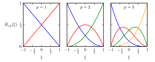
Figure 8: The Bernstein basis for polynomial degrees $p=1,2,3$.

We construct a bivariate Bernstein basis function of degree $\mathbf{p}=\{p,q\}$ by $B_{a,\mathbf{p}}:\bar{\Omega}\rightarrow\mathbb{R}^{+}\cup 0$ where $a=1,\ldots,n_{b}$, $n_{b}=(p+1)(q+1)$, and $\bar{\Omega}=[-1,1]^{2}$, as the tensor product of univariate basis functions

$$B_{a(i,j),\mathbf{p}}(\xi,\eta)=B_{i,p}(\xi)B_{j,q}(\eta)$$ (8)

with

$$a\left(i,j\right)=(p+1)(j-1)+i.$$ (9)

6.2 The geometry of a hierarchical representation

In a single level T-spline, basis functions and control points have a one-to-one relationship and each control point influences the geometry in a similar manner. In a hierarchical context it is common to only associate control points with the functions in $\mathsf{N}^{1}$. This is the convention adopted in this paper. Note that by construction every blending function in $\mathsf{N}^{1}$ can be written in terms of basis functions in $\mathsf{H}$ (see Lemma 5.4). We call the functions in $\mathsf{N}^{1}$ geometric blending functions. We use $n_{g}$ to denote the number of geometric blending functions.

Given vector valued control points, $\mathbf{P}_{G}\in\mathbb{R}^{n}$, $n=2$ or $3$, and weights $w_{G}$, the geometry of a hierarchical representation $\mathbf{x}:\hat{\Omega}\rightarrow\Omega$ can be written as

$$\mathbf{x}(s,t) =\frac{\sum_{G=1}^{n_{g}}\mathbf{P}_{G}w_{G}N_{G}(s,t)}{\sum_{G=1}^{n_{g}}w_{G}N_{G}(s,t)}$$ (10)

$$=\frac{\sum_{G=1}^{n_{g}}\mathbf{P}_{G}w_{G}N_{G}(s,t)}{w(s,t)}$$ (11)

where $(s,t)\in\hat{\Omega}$, $G$ is used to index the geometric blending functions, and $w(s,t)$ is the weight function. The decoupling of geometry from the basis functions in $\mathsf{H}$ is an additional complexity unique to hierarchical representations which is elegantly addressed via Bézier extraction.

6.3 Bézier Elements

The set of Bézier elements underlying a hierarchical T-spline are determined recursively in a manner similar to the basis. We denote the set of Bézier elements in a hierarchy by $\mathsf{HE}$. We construct $\mathsf{HE}$ as follows:

1. Initialize $\mathsf{HE}^{1}=\mathsf{E}^{1}.$

2. Recursively construct $\mathsf{HE}^{\alpha+1}$ from $\mathsf{HE}^{\alpha}$ by setting

   $$\mathsf{HE}^{\alpha+1}=\mathsf{HE}^{\alpha+1}_{coarse}\cup\mathsf{HE}^{\alpha+1}_{fine},\alpha=1,\ldots,N-1,$$

   where

   $$\mathsf{HE}^{\alpha+1}_{coarse}=\{e\in\mathsf{HE}^{\alpha}:\hat{\Omega}^{e}\nsubseteq\hat{\Omega}^{\alpha+1}\},$$

   and

   $$\mathsf{HE}^{\alpha+1}_{fine}=\{e\in\mathsf{E}^{\alpha+1}:\hat{\Omega}^{e}\subseteq\hat{\Omega}^{\alpha+1}\}.$$

3. Set $\mathsf{HE}=\mathsf{HE}^{N}.$

We denote the number of Bézier elements in $\mathsf{HE}$ by $n_{e}$.

6.4 Element localization

Using standard techniques [29, 61] it is possible to determine the set of functions in $\mathsf{H}$ which are nonzero over any element in $\mathsf{HE}$. This gives rise to a standard element connectivity map which, given an element index $e$ and local function index $a$, returns a global function index $A$. In other words $A=\operatorname{IEN}(e,a)$. The reader is referred to [56] for additional details on common approaches to finite element localization and the $\operatorname{IEN}$ array. Note that $A$ can indicate an anchor or a global function index.

We write a rational hierarchical T-spline basis function, restricted to element $e$, as

$$R_{a}^{e}(s,t) =\frac{N_{a}^{e}(s,t)}{w^{e}(s,t)}$$ (12)

where $(s,t)\in\hat{\Omega}^{e}$ and $w^{e}(s,t)$ is the element weight function restricted to element $e$. The element geometric map $\mathbf{x}^{e}:\hat{\Omega}^{e}\rightarrow\Omega^{e}$ is the restriction of $\mathbf{x}(s,t)$ to element $e$.

6.5 Bézier extraction

To present the basic ideas, Bézier extraction for a B-spline curve is shown graphically in Figure 9. Bézier extraction constructs a linear transformation defined by a matrix referred to as the extraction operator. The extraction operator maps a Bernstein polynomial basis defined on Bézier elements to the global spline basis. The transpose of the extraction operator maps the control points of the spline to the Bézier control points.

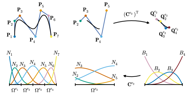
Figure 9: Illustration of the Bézier extraction operator $\mathbf{C}^{e}$ for a spline of degree 3.

Each hierarchical basis function supported by element $e$ can be written in Bézier form as

$$N_{a}^{e}(s({\xi}),t(\eta)) =\sum_{b=1}^{n_{b}}c^{a}_{b}B_{b}(\xi,\eta)$$ (13)

$$=\bar{N}_{a}^{e}(\xi,\eta)$$ (14)

where the dependence of the Bernstein polynomial $B_{b}(\xi,\eta)$ on the polynomial degrees $p$ and $q$ has been suppressed for clarity. The overbar will be used to denote a quantity written in terms of the Bernstein basis defined over the element domain $\bar{\Omega}$. The Bézier coefficients $c^{a}_{b}$ are computed using standard knot insertion techniques [29]. We denote the vector of hierarchical basis functions supported by element $e$ by $\mathbf{H}^{e}(\xi,\eta)$ and the vector of Bernstein basis functions by $\mathbf{B}(\xi,\eta)$. We then have that

$$\mathbf{N}^{e}(s(\xi),t(\eta)) =\mathbf{C}^{e}\mathbf{B}(\xi,\eta)$$ (15)

$$=\bar{\mathbf{N}}^{e}(\xi,\eta)$$ (16)

where $\mathbf{C}^{e}$ is the element extraction operator (see  [9]). In other words, the element extraction operator is composed of the Bézier coefficients $c_{b}^{a}$.

We write the element weight function as

$$w^{e}(s(\xi),t(\eta)) =\sum_{g=1}^{n_{g}^{e}}w_{g}^{e}N_{g}^{e}(s(\xi),t(\eta))$$

$$=\sum_{g=1}^{n_{g}^{e}}w_{g}^{e}\sum_{b=1}^{n_{b}}c^{g}_{b}B_{b}(\xi,\eta)$$

$$=\sum_{b=1}^{n_{b}}\left(\sum_{g=1}^{n_{g}^{e}}w_{g}^{e}c^{g}_{b}\right)B_{b}(\xi,\eta)$$

$$=\sum_{b=1}^{n_{b}}w_{b}^{e}B_{b}(\xi,\eta)$$

$$=\bar{w}^{e}(\xi,\eta).$$

where $n_{g}^{e}$ is the number of geometric basis functions which are non-zero over element $e$. We may also write the rational hierarchical basis functions as

$$R_{a}^{e}(s(\xi),t(\eta)) =\frac{N_{a}^{e}(s(\xi),t(\eta))}{w^{e}(s(\xi),t(\eta))}$$

$$=\frac{\bar{N}_{a}^{e}(\xi,\eta)}{\bar{w}^{e}(\xi,\eta)}$$

$$=\bar{R}_{a}^{e}(\xi,\eta).$$

Finally, the element geometric map can be written as

$$\mathbf{x}^{e}(s(\xi),t(\eta)) =\frac{\sum_{g=1}^{n^{e}_{g}}\mathbf{P}_{g}^{e}w_{g}^{e}N_{g}^{e}(s(\xi),t(\eta))}{w^{e}(s(\xi),t(\eta))}$$

$$=\frac{\sum_{g=1}^{n^{e}_{g}}\mathbf{P}_{g}^{e}w_{g}^{e}\sum_{b=1}^{n_{b}}c^{g}_{b}B_{b}(\xi,\eta)}{\bar{w}^{e}(\xi,\eta)}$$

$$=\frac{\sum_{b=1}^{n_{b}}\left(\sum_{g=1}^{n^{e}_{g}}\mathbf{P}_{g}^{e}w_{g}^{e}c^{g}_{b}\right)B_{b}(\xi,\eta)}{\bar{w}^{e}(\xi,\eta)}$$

$$=\frac{\sum_{b=1}^{n_{b}}\mathbf{Q}_{b}^{e}w_{b}^{e}B_{b}(\xi,\eta)}{\bar{w}^{e}(\xi,\eta)}$$

$$=\bar{\mathbf{x}}^{e}(\xi,\eta).$$

The implementation of a finite element framework based on Bézier extraction is described in detail in [29, 61].

7 Computational Results

We illustrate the use of hierarchical T-splines in the context of isogeometric analysis. We consider problems that highlight the unique attributes of both hierarchical refinement and T-splines. The examples used are inspired by those found in [2, 8, 9].

7.1 A comparison between ASTS and HASTS local refinement

We compare local refinement of ASTS to local refinement of HASTS. When working with ASTS all refinement is performed on a single level whereas when working with HASTS this constraint is relaxed. For additional algorithmic details on local refinement of ASTS see [2]. We locally refine the T-spline ship hull design shown in Fig. 10 using both methods. The geometry is constructed using the Autodesk T-spline plugin for Rhino3d [62]. T-splines are popular in ship hull design because an entire hull can be modeled by a single watertight surface with a minimal number of control points [63]. T-junctions can be used to efficiently model local features. Note that the initial T-spline of the hull contains just $75$ control points and $36$ Bézier elements.

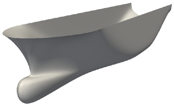
Figure 10: A T-spline container ship hull. The surface is $C^{2}$-continuous everywhere.

We restrict the refinement region to the locations detailed in Fig. 11. It is assumed that the original design is too coarse to be used as a basis for analysis and additional resolution is required in the rectangular region followed by highly localized refinements along the region corresponding to the curve.

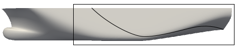
Figure 11: The regions of the container ship hull where local refinement will be performed. Refinement is first performed in the rectangular region followed by highly localized refinement along the curve.

The HASTS refinement algorithm is based on the algorithm presented in [9] for spline forests. The algorithm is element-based, meaning refinement is driven by the subdivision of Bézier elements. The hierarchical basis is then reextracted into the new hierarchical T-mesh topology to generate the new set of Bézier elements. A detailed description of the underlying algorithms, in the context of HASTS, will be postponed to a future publication. Figure 12 shows three HASTS local refinements along the curve shown in Figure 11. The elements are colored according to their level, $\alpha$, in the hierarchy. Note that no nonlocal propagation of local refinement occurs for HASTS. Only those elements specified for refinement are subdivided. This is possible due to the relaxation of the single level constraint inherent in ASTS. The refinements form a nested sequence of $C^{2}$-continuous hierarchical analysis-suitable T-spline spaces. The geometry of the hull is exactly preserved during refinement. The final HASTS is composed of $1857$ Bézier elements and $1193$ basis functions. However, only $75$ geometric blending functions and control points are used to define the hull geometry.

Figure 12: Three iterations of HASTS local refinement along the curve for the container ship hull in Figure 10. The elements are colored according to their level, $\alpha$, in the hierarchy. The refinements form a nested sequence of $C^{2}$-continuous hierarchical analysis-suitable T-spline spaces. The geometry of the hull is exactly preserved during refinement.

As a comparison, Figure 13 shows the results of ASTS local refinement using the algorithm from [2]. The top figure shows the control points added during local refinement (black dots) along the curve. The region selected for refinement is shown in red. Observe the propagation of the control points away from the selected refinement region. The bottom figure shows the resulting Bézier elements after refinement. Superfluous control points and elements are added just to satisfy the single level constraint inherent in the definition of ASTS.

Figure 13: The results of ASTS local refinement using the algorithm from [2]. The top figure shows the control points added during local refinement (black dots) along the curve. Observe the propagation of the control points away from the selected refinement region. The bottom figure shows the resulting Bézier elements after refinement. Superfluous control points and elements are added just to satisfy the single level constraint inherent in the definition of ASTS.

7.2 HASTS as an adaptive basis

We now consider HASTS as an adaptive basis for isogeometric analysis. We choose as a benchmark the advection skew to the mesh problem shown in Figure 14. This problem is advection dominated, with diffusivity of $10^{-6}$. Along the external boundary, the boundary conditions are selected such that sharp interior and boundary layers are present in the solution. In this case, $\theta=45$ degrees.

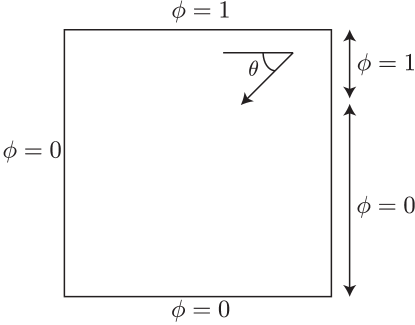
Figure 14: The advection skew to the mesh problem statement.

7.2.1 Problem Statement

Let $\Omega$ be a bounded region in $\mathbb{R}^{2}$ and assume $\Omega$ has a piecewise smooth boundary $\Gamma$. Let $\mathbf{x}=\{x_{i}\}_{i=1}^{2}$ denote a general point in $\overline{\Omega}$, and let the temperature at a point $\mathbf{x}\in\Omega$ be denoted by $\phi(\mathbf{x})\in\mathbb{R}$. Given Dirichlet boundary data, $g:\Gamma\rightarrow\mathbb{R}$, the steady-state advection-diffusion boundary value problem consists of finding the temperature $\phi$ such that

$$\mathbf{u}\cdot\nabla\phi-\nabla\cdot\left(\boldsymbol{\kappa}\nabla\phi\right) =0\text{ on $\Omega$}$$ (17)

$$\phi =g\text{ on $\Gamma$}$$

where $\mathbf{u}:\Omega\rightarrow\mathbb{R}^{2}$ and $\boldsymbol{\kappa}:\Omega\rightarrow\mathbb{R}^{2\times 2}$ are the spatially varying solenoidal velocity vector and symmetric, positive-definite, diffusivity tensor, respectively. Note that in this paper we define $\boldsymbol{\kappa}=\kappa\delta_{ij}$ where $\kappa$ is a positive constant called the diffusivity coefficient. We employ SUPG [64] with a standard definition for the element stabilization parameter, $\tau^{e}$.

7.2.2 A residual based error estimator

To estimate the error we employ a simple residual-based explicit estimator based on the variational multiscale theory for fluids [65, 66, 67, 68]. It is given by

$$||\phi^{\prime}||_{\Omega^{e}}\approx\tau^{e}||\mathbf{u}\cdot\nabla\phi-\nabla\cdot\boldsymbol{\kappa}\nabla\phi||_{\Omega^{e}}.$$ (18)

Note that this error estimator underestimates the error for diffusion-dominated flows but is adequate for the advection-dominated benchmark presented in this paper. Using standard techniques [56] we use the element scaling

$$r=\frac{h^{e}_{\alpha+1}}{h^{e}_{\alpha}}=\left(\frac{tol}{||\phi^{\prime}||_{\Omega^{e}}}\right)^{\nicefrac{{1}}{{\beta}}}$$ (19)

where $h^{e}_{\alpha},h^{e}_{\alpha+1}$ are the mesh size distributions for $\mathsf{T}^{\alpha}$ and $\mathsf{T}^{\alpha+1}$, respectively, and $\beta$ is the order of convergence of the method. The element size, $h^{e}$, is the square root of the element area. We flag elements for refinement if $r<1$. The adaptive process is repeated until a specified convergence tolerance is attained or a maximum number of hierarchical levels are introduced.

7.3 Results

We solve the problem with $C^{1}$ biquadratic and $C^{2}$ bicubic hierarchical T-splines. The initial T-mesh for both cases is shown in Figure 15. Note that the initial T-mesh is locally refined to accommodate the presence of sharp boundary layers in the solution. Note that this refinement is not hierarchical. We have found that judiciously performing local refinement of the first level of a T-spline hierarchy to accommodate geometric features or boundary conditions leads to smaller hierarchies and more efficient solution procedures.

During each adaptive step the error is assessed as described in Section 7.2.2, elements are flagged for refinement and subdivided, and a new hierarchical basis is then extracted into the new hierarchical T-mesh topology. This generates a refined set of Bézier elements. The sequence of Bézier mesh refinements is shown for both the biquadratic and bicubic case in Figures 16–17. The sequence of biquadratic refinements form a nested sequence of $C^{1}$-continuous HASTS spaces, whereas the sequence of bicubic refinements form a nested sequence of $C^{2}$-continuous HASTS spaces. Note that fewer elements are required for convergence as the smoothness and order of the basis increases [9].

To illustrate the structure and distribution of the hierarchical basis the Greville abscissae [23] are plotted in Figures 18–20. Note that a linear parameterization was employed for all meshes and the level zero control points and blending functions define the geometry. The dots are scaled according to their level in the hierarchy; a larger dot denotes a lower level. The sequence of solutions are shown in Figures 21–22.

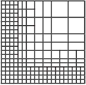
Figure 15: Initial T-mesh for the static advection skew to the mesh problem.

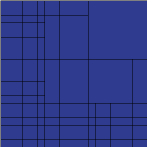
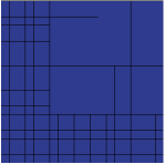
(a) Initial biquadratic Bézier mesh	(b) Initial bicubic Bézier mesh
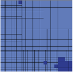
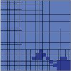
(c) Second biquadratic Bézier mesh	(d) Second bicubic Bézier mesh
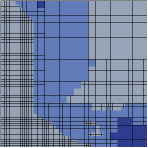
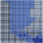
(e) Third biquadratic Bézier mesh	(f) Third bicubic Bézier mesh

Figure 16: The first two iterations of HASTS local refinement for the biquadratic (left column) and bicubic (right column) advection skew to the mesh problem. The elements are colored according to their level, $\alpha$, in the hierarchy. The biquadratic refinements form a nested sequence of $C^{1}$-continuous HASTS spaces and the bicubic refinements form a nested sequence of $C^{2}$-continuous HASTS spaces.

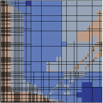
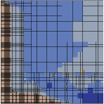
(a) Fourth biquadratic Bézier mesh	(b) Fourth bicubic Bézier mesh
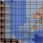
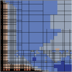
(c) Fifth biquadratic Bézier mesh	(d) Fifth bicubic Bézier mesh
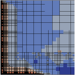
(e) Sixth biquadratic Bézier mesh	(f) Sixth bicubic Bézier mesh

Figure 17: The third through fifth iterations of HASTS local refinement for the biquadratic (left column) and bicubic (right column) advection skew to the mesh problem. The elements are colored according to their level, $\alpha$, in the hierarchy.

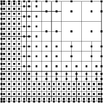
(a) Initial quadratic Greville abscissae	(b) Initial bicubic Greville abscissae
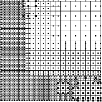
(c) Greville abscissae for second biquadratic mesh	(d) Greville abscissae for second bicubic mesh

Figure 18: The Greville abscissae (black dots) corresponding to the basis functions for the first two iterations of HASTS local refinement for the biquadratic (left column) and bicubic (right column) advection skew to the mesh problem. The size of the dot corresponds to the basis function level with larger dots corresponding to lower levels.

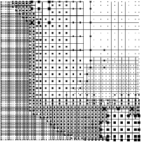
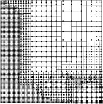
(a) Greville abscissae for third biquadratic mesh	(b) Greville abscissae for third bicubic mesh
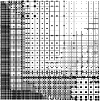
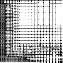
(c) Greville abscissae for fourth biquadratic mesh	(d) Greville abscissae for fourth bicubic mesh

Figure 19: The Greville abscissae (black dots) corresponding to the basis functions for the third and fourth iterations of HASTS local refinement for the biquadratic (left column) and bicubic (right column) advection skew to the mesh problem. The size of the dot corresponds to the basis function level with larger dots corresponding to lower levels.

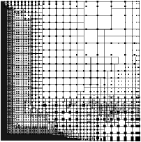
(a) Greville abscissae for fifth biquadratic mesh	(b) Greville abscissae for fifth bicubic mesh
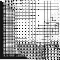
(c) Greville abscissae for sixth biquadratic mesh	(d) Greville abscissae for sixth bicubic mesh

Figure 20: The Greville abscissae (black dots) corresponding to the basis functions for the fifth and sixth iterations of HASTS local refinement for the biquadratic (left column) and bicubic (right column) advection skew to the mesh problem. The size of the dot corresponds to the basis function with larger dots corresponding to lower levels.

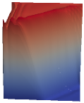
(a) Solution 1 (b) Solution 2 (c) Solution 3 (d) Solution 4

(f) Solution 5

Figure 21: Quadratic solutions to the advection skew to the mesh problem. These solutions correspond to the Bézier meshes in the left column of Figures 16–17.

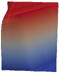
(a) Solution 1 (b) Solution 2 (c) Solution 3 (d) Solution 4

(f) Solution 5

Figure 22: Cubic solutions to the advection skew to the mesh problem. These solutions correspond to the Bézier meshes in the right column of Figures 16–17.

8 Conclusion

We have presented hierarchical analysis-suitable T-splines which is a superset of both analysis-suitable T-splines and hierarchical B-splines. We have also developed the necessary theoretical formulation of HASTS including a proof of the local linear independence of analysis-suitable T-splines. We presented a simple algorithm for the creation of nested T-spline spaces and also extended Bézier extraction to HASTS. We then demonstrated the potential of HASTS by comparing HASTS to a local refinement algorithm for T-splines which demonstrated the improved efficiency and locality of using a hierarchical approach. We also demonstrated the use of HASTS in the context of isogeometric analysis by solving the benchmark static skew advection problem.

In future work we will provide a detailed description of the underlying algorithms to perform hierarchical refinement in the context of HASTS. We will also consider hierarchical $p$ and $k$ refinements of T-splines. Finally, we intend to extend the definition of spline forests in [9] to the T-spline regime. This will allow us to accommodate smooth interfaces and also interface directly with commercial T-spline products.

References

- [1] X. Li, J. Zheng, T. W. Sederberg, T. J. R. Hughes, M. A. Scott, On linear independence of T-spline blending functions, Computer Aided Geometric Design 29 (2012) 63 – 76.
- [2] M. A. Scott, X. Li, T. W. Sederberg, T. J. R. Hughes, Local refinement of analysis-suitable T-splines, Computer Methods in Applied Mechanics and Engineering 213 (2012) 206 – 222.
- [3] L. Beirão da Veiga, A. Buffa, D. Cho, G. Sangalli, Analysis-suitable T-splines are dual-compatible, Computer Methods in Applied Mechanics and Engineering 249 – 252 (2012) 42 – 51.
- [4] L. B. da Veiga, A. Buffa, G. Sangalli, R. Vázquez, Analysis-suitable T-splines of arbitrary degree: definition, linear independence, and approximation properties, Mathematical Models and Methods in Applied Sciences 23 (11) (2013) in press.
- [5] X. Li, M. A. Scott, Analysis-suitable T-splines: characterization, refineability, and approximation, Mathematical Models and Methods in Applied Science 24 (06) (2014) 1141–1164.
- [6] D. R. Forsey, R. H. Bartels, Hierarchical B-spline refinement, ACM SIGGRAPH Computer Graphics 22 (4) (1988) 205–212.
- [7] D. Schillinger, L. Dedé, M. A. Scott, J. A. Evans, M. J. Borden, E. Rank, T. J. R. Hughes, An isogeometric design-through-analysis methodology based on adaptive hierarchical refinement of NURBS, immersed boundary methods, and T-spline CAD surfaces, Computer Methods in Applied Mechanics and Engineering 249 – 252 (2012) 116 – 150.
- [8] A. Vuong, C. Giannelli, B. Jüttler, B. Simeon, A hierarchical approach to adaptive local refinement in isogeometric analysis, Computer Methods in Applied Mechanics and Engineering 200 (49 – 52) (2011) 3554 – 3567.
- [9] M. A. Scott, D. T. Thomas, E. J. Evans, Isogeometric spline forests, Computer Methods in Applied Mechanics and Engineering 269 (2014) 222 – 264.
- [10] C. Giannelli, B. Jüttler, Bases and dimensions of bivariate hierarchical tensor-product splines, Journal of Computational and Applied Mathematics 239 (0) (2013) 162 – 178.
- [11] C. Giannelli, B. Jüttler, H. Speleers, THB–splines: The truncated basis for hierarchical splines, Computer Aided Geometric Design 29 (7) (2012) 485 – 498.
- [12] T. W. Sederberg, J. Zheng, A. Bakenov, A. Nasri, T-splines and T-NURCCs, ACM Trans. Graph. 22 (2003) 477–484.
- [13] T. W. Sederberg, D. L. Cardon, G. T. Finnigan, N. S. North, J. Zheng, T. Lyche, T-spline simplification and local refinement, ACM Trans. Graph. 23 (2004) 276–283.
- [14] Autodesk, Autodesk T-Splines Plug-in for Rhino user manual, Autodesk (2012).
- [15] Autodesk, Inc., Autodesk Fusion 360, Autodesk, Inc. (2014).
- [16] T. J. R. Hughes, J. A. Cottrell, Y. Bazilevs, Isogeometric analysis: CAD, finite elements, NURBS, exact geometry, and mesh refinement, Computer Methods in Applied Mechanics and Engineering 194 (2005) 4135–4195.
- [17] J. A. Cottrell, T. J. R. Hughes, Y. Bazilevs, Isogeometric analysis: Toward Integration of CAD and FEA, Wiley, Chichester, 2009.
- [18] J. A. Evans, Y. Bazilevs, I. Babuška, T. J. R. Hughes, n-widths, sup-infs, and optimality ratios for the k-version of the isogeometric finite element method, Computer Methods in Applied Mechanics and Engineering 198 (21-26) (2009) 1726–1741.
- [19] T. J. R. Hughes, J. A. Evans, A. Reali, Finite element and NURBS approximations of eigenvalue, boundary-value, and initial-value problems, Computer Methods in Applied Mechanics and Engineering 272 (2014) 290 – 320.
- [20] J. A. Cottrell, T. J. R. Hughes, A. Reali, Studies of refinement and continuity in isogeometric analysis, Computer Methods in Applied Mechanics and Engineering 196 (2007) 4160–4183.
- [21] W. Wang, Y. Zhang, M. A. Scott, T. J. R. Hughes, Converting an unstructured quadrilateral mesh to a standard T-spline surface, Computational Mechanics, 48 (2011) 477 – 498.
- [22] L. Liu, Y. Zhang, T. J. R. Hughes, M. A. Scott, T. W. Sederberg, Volumetric T-spline construction using boolean operations, in: J. Sarrate, M. Staten (Eds.), Proceedings of the 22nd International Meshing Roundtable, Springer International Publishing, 2014, pp. 405–424.
- [23] M. A. Scott, R. N. Simpson, J. A. Evans, S. Lipton, S. P. A. Bordas, T. J. R. Hughes, T. W. Sederberg, Isogeometric boundary element analysis using unstructured T-splines, Computer Methods in Applied Mechanics and Engineering 254 (2013) 197 – 221.
- [24] R. Schmidt, R. Wüchner, K.-U. Bletzinger, Isogeometric analysis of trimmed NURBS geometries, Computer Methods in Applied Mechanics and Engineering 241–244 (2012) 93 – 111.
- [25] D. J. Benson, Y. Bazilevs, E. De Luycker, M. C. Hsu, M. A. Scott, T. J. R. Hughes, T. Belytschko, A generalized finite element formulation for arbitrary basis functions: From isogeometric analysis to XFEM, International Journal for Numerical Methods in Engineering 83 (2010) 765–785.
- [26] W. A. Wall, M. A. Frenzel, C. Cyron, Isogeometric structural shape optimization, Computer Methods in Applied Mechanics and Engineering 197 (2008) 2976–2988.
- [27] Y. Bazilevs, V. M. Calo, J. A. Cottrell, J. A. Evans, T. J. R. Hughes, S. Lipton, M. A. Scott, T. W. Sederberg, Isogeometric analysis using T-splines, Computer Methods in Applied Mechanics and Engineering 199 (5-8) (2010) 229–263.
- [28] M. Dörfel, B. Jüttler, B. Simeon, Adaptive isogeometric analysis by local h-refinement with T-splines, Computer Methods in Applied Mechanics and Engineering 199 (5–8) (2009) 264–275.
- [29] M. A. Scott, M. J. Borden, C. V. Verhoosel, T. W. Sederberg, T. J. R. Hughes, Isogeometric Finite Element Data Structures based on Bézier Extraction of T-splines, International Journal for Numerical Methods in Engineering, 88 (2011) 126 – 156.
- [30] C. V. Verhoosel, M. A. Scott, T. J. R. Hughes, R. de Borst, An isogeometric analysis approach to gradient damage models, International Journal for Numerical Methods in Engineering, 86 (2011) 115–134.
- [31] C. V. Verhoosel, M. A. Scott, R. de Borst, T. J. R. Hughes, An isogeometric approach to cohesive zone modeling, International Journal for Numerical Methods in Engineering, 87 (2011) 336 – 360.
- [32] M. J. Borden, M. A. Scott, C. V. Verhoosel, C. M. Landis, T. J. R. Hughes, A phase-field description of dynamic brittle fracture, Computer Methods in Applied Mechanics and Engineering 217 (2012) 77 – 95.
- [33] R. Simpson, M. Scott, M. Taus, D. Thomas, H. Lian, Acoustic isogeometric boundary element analysis, Computer Methods in Applied Mechanics and Engineering 269 (2014) 265–290.
- [34] R. Dimitri, L. D. Lorenzis, M. A. Scott, P. Wriggers, R. Taylor, G. Zavarise, Isogeometric large deformation frictionless contact using T-splines, Computer methods in applied mechanics and engineering 269 (2014) 394 – 414.
- [35] S. Hosseini, J. J. Remmers, C. V. Verhoosel, R. de Borst, An isogeometric continuum shell element for non-linear analysis, Computer Methods in Applied Mechanics and Engineering 271 (2014) 1 – 22.
- [36] Y. Bazilevs, M. C. Hsu, M. A. Scott, Isogeometric fluid-structure interaction analysis with emphasis on non-matching discretizations, and with application to wind turbines, Computer Methods in Applied Mechanics and Engineering 249 - 252 (2012) 28 – 41.
- [37] A. Buffa, G. Sangalli, R. Vázquez, Isogeometric methods for computational electromagnetics: B-spline and T-spline discretizations, Journal of Computational Physics 257, Part B (2014) 1291 – 1320.
- [38] A. I. Ginnis, K. V. Kostas, C. G. Politis, P. D. Kaklis, K. A. Belibassakis, T. P. Gerostathis, M. A. Scott, T. J. R. Hughes, Isogeometric boundary-element analysis for the wave-resistance problem using T-splines, Computer Methods in Applied Mechanics and Engineering submitted.
- [39] G. Kuru, C. Verhoosel, K. van der Zee, E. van Brummelen, Goal-adaptive isogeometric analysis with hierarchical splines, Computer Methods in Applied Mechanics and Engineering 270 (2014) 270 – 292.
- [40] D. Schillinger, J. A. Evans, A. Reali, M. A. Scott, T. J. R. Hughes, Isogeometric collocation: Cost comparison with Galerkin methods and extension to adaptive hierarchical NURBS discretizations, Computer Methods in Applied Mechanics and Engineering 267 (2013) 170 – 232.
- [41] E. Grinspun, P. Krysl, P. Schröder, CHARMS: a simple framework for adaptive simulation, ACM Transactions on Graphics 21 (3) (2002) 281–290.
- [42] D. Schillinger, E. Rank, An unfitted -adaptive finite element method based on hierarchical B-splines for interface problems of complex geometry, Computer Methods in Applied Mechanics and Engineering 200 (47–48) (2011) 3358 – 3380.
- [43] G. Kiss, C. Giannelli, B. Jüttler, Algorithms and data structures for truncated hierarchical B-splines, in: M. Floater, T. Lyche, M.-L. Mazure, K. Mørken, L. Schumaker (Eds.), Mathematical Methods for Curves and Surfaces, Vol. 8177 of Lecture Notes in Computer Science, Springer Berlin Heidelberg, 2014, pp. 304–323.
- [44] C. Giannelli, B. Jüttler, H. Speleers, Strongly stable bases for adaptively refined multilevel spline spaces, Advances in Computational Mathematics (2013) 1–32.
- [45] D. Berdinsky, T. wan Kim, C. Bracco, D. Cho, B. Mourrain, M. Oh, S. Kiatpanichgij, Dimensions and bases of hierarchical tensor-product splines, Journal of Computational and Applied Mathematics 257 (2014) 86 – 104.
- [46] J. Deng, F. Chen, X. Li, C. Hu, W. Tong, Z. Yang, Y. Feng, Polynomial splines over hierarchical T-meshes, Graphical Models 74 (2008) 76–86.
- [47] X. Li, J. Deng, F. Chen, Surface modeling with polynomial splines over hierarchical T-meshes, The Visual Computer 23 (2007) 1027–1033.
- [48] X. Li, J. Deng, F. Chen, Polynomial splines over general T-meshes, The Visual Computer 26 (2010) 277–286.
- [49] X. Li, J. Deng, F. Chen, The dimension of spline spaces over 3d hierarchical T-meshes, Journal of Information and Computational Science 3 (2006) 487–501.
- [50] H. Kang, F. Chen, J. Deng, Modified T-splines, Computer Aided Geometric Design 30 (9) (2013) 827 – 843.
- [51] T. Dokken, T. Lyche, K. F. Pettersen, Polynomial splines over locally refined box-partitions, Computer Aided Geometric Design 30 (3) (2013) 331–356.
- [52] A. Bressan, Some properties of LR-splines, Computer Aided Geometric Design 30 (8) (2013) 778 – 794.
- [53] C. Manni, F. Pelosi, M. L. Sampoli, Generalized B-splines as a tool in isogeometric analysis, Computer Methods in Applied Mechanics and Engineering 200 (5–8) (2011) 867 – 881.
- [54] P. Costantini, C. Manni, F. Pelosi, M. L. Sampoli, Quasi-interpolation in isogeometric analysis based on generalized B-splines, Computer Aided Geometric Design 27 (8) (2010) 656–668.
- [55] C. Bracco, D. Berdinsky, D. Cho, M. Oh, T. wan Kim, Trigonometric generalized T-splines, Computer Methods in Applied Mechanics and Engineering 268 (2014) 540 – 556.
- [56] T. J. R. Hughes, The Finite Element Method: Linear Static and Dynamic Finite Element Analysis, Dover Publications, Mineola, NY, 2000.
- [57] G. E. Farin, NURBS Curves and Surfaces: from Projective Geometry to Practical Use, A. K. Peters, Ltd., Natick, MA, 1999.
- [58] T. W. Sederberg, Computer Aided Geometric Design: Course Notes, http://www.tsplines.com/educationportal.html (2010).
- [59] L. Ramshaw, Blossoms are polar forms, Computer Aided Geometric Design 6 (4) (1989) 323–358.
- [60] L. Schumaker, Spline functions: basic theory, Krieger, 1993.
- [61] M. J. Borden, M. A. Scott, J. A. Evans, T. J. R. Hughes, Isogeometric finite element data structures based on Bézier extraction of NURBS, International Journal for Numerical Methods in Engineering, 87 (2011) 15 – 47.
- [62] Autodesk, Inc., http://www.tsplines.com/rhino/ (2011).
- [63] M. T. Sederberg, T. W. Sederberg, T-splines: A technology for marine design with minimal control points, http://www.tsplines.com/technicalpapers.html (2010).
- [64] A. N. Brooks, T. J. R. Hughes, Streamline upwind / Petrov-Galerkin formulations for convection dominated flows with particular emphasis on the incompressible Navier-Stokes equations, Computer Methods in Applied Mechanics and Engineering 32 (1982) 199–259.
- [65] T. J. R. Hughes, Multiscale phenomena: Green’s functions, the Dirichlet-to-Neumann formulation, subgrid scale models, bubbles and the origins of stabilized methods, Computer Methods in Applied Mechanics and Engineering 127 (1995) 387–401.
- [66] M. G. Larson, A. Målqvist, Adaptive variational multiscale methods based on a posteriori error estimation: Duality techniques for elliptic problems, in: B. Engquist, O. Runborg, P. Lötstedt (Eds.), Multiscale Methods in Science and Engineering, Vol. 44 of Lecture Notes in Computational Science and Engineering, Springer Berlin Heidelberg, 2005, pp. 181–193.
- [67] G. Hauke, M. H. Doweidar, M. Miana, The multiscale approach to error estimation and adaptivity, Computer Methods in Applied Mechanics and Engineering 195 (13–16) (2006) 1573 – 1593.
- [68] G. Hauke, M. H. Doweidar, S. Fuentes, Mesh adaptivity for the transport equation led by variational multiscale error estimators, International Journal for Numerical Methods in Fluids 69 (12) (2012) 1835–1850.