A 3D radiative transfer framework: XI. multi-level NLTE

Abstract

Context. Multi-level non-local thermodynamic equilibrium (NLTE) radiation transfer calculations have become standard throughout the stellar atmospheres community and are applied to all types of stars as well as dynamical systems such as novae and supernovae. Nevertheless even today spherically symmetric 1D calculations with full physics are computationally intensive. We show that full physics NLTE calculations can be done with fully 3 dimensional (3D) radiative transfer.

Aims. With modern computational techniques and current massive parallel computational resources, full detailed solution of the multi-level NLTE problem coupled to the solution of the radiative transfer scattering problem can be solved without sacrificing the micro physics description.

Methods. We extend the use of a rate operator developed to solve the coupled NLTE problem in spherically symmetric 1D systems. In order to spread memory among processors we have implemented the NLTE/3D module with a hierarchical domain decomposition method that distributes the NLTE levels, radiative rates, and rate operator data over a group of processes so that each process only holds the data for a fraction of the voxels. Each process in a group holds all the relevant data to participate in the solution of the 3DRT problem so that the 3DRT solution is parallelized within a domain decomposition group.

Results. We solve a spherically symmetric system in 3D spherical coordinates in order to directly compare our well-tested 1D code to the 3D case. We compare three levels of tests: a) a simple H+He test calculation, b) H+He+CNO+Mg, c) H+He+Fe. The last test is computationally large and shows that realistic astrophysical problems are solvable now, but they do require significant computational resources.

Conclusions. With presently available computational resources it is possible to solve the full 3D multi-level problem with the same detailed micro-physics as included in 1D modeling.

1 Introduction

In a series of papers Hauschildt & Baron (2006, hereafter: Papers I–X); Baron & Hauschildt (2007, hereafter: Papers I–X); Hauschildt & Baron (2008, 2009, hereafter: Papers I–X); Baron, Hauschildt, & Chen (2009, hereafter: Papers I–X); Seelmann, Hauschildt, & Baron (2010, hereafter: Papers I–X); Hauschildt & Baron (2011, hereafter: Papers I–X); Jack, Hauschildt, & Baron (2012, hereafter: Papers I–X); Baron, Hauschildt, Chen, & Knop (2012, hereafter: Papers I–X), we have described a framework for the solution of the radiative transfer equation in 3D systems (3DRT), including a detailed treatment of scattering in continua and lines with a non-local operator splitting method. In Hauschildt & Baron (2010) we described tests of the 3D mode of the PHOENIX model atmosphere code package.

Here, we describe the implementation and the results of detailed multi-level non-local thermodynamic equilibrium (NLTE) PHOENIX/3D calculations and compare the results to equivalent 1D calculations with PHOENIX/1D models. We will first describe the method we have implemented and discuss differences to the 1D version, then we will show and discuss the results of simple test calculations.

As 3D hydrodynamical calculations become more common, detailed radiative transfer effects due to the 3D structure will be needed in order to directly compare the predictions of hydrodynamic results with observations. 3D effects due to convective structure are known to be important in the sun and other stars (Hayek et al. 2011; Asplund et al. 2005; Asplund 2000; Asplund et al. 2000, 1999). It is also known that NLTE effects can play an important role (Bergemann et al. 2012). This is also the case for brown dwarfs, irradiated planets, and circumstellar disks (Hügelmeyer et al. 2009; Wawrzyn et al. 2009; Witte et al. 2011). 3D radiative transfer effects play a role in interpreting the spectra of active stars (Berkner et al. 2013). In addition, 3D radiative transfer effects are important in the binary environment of Type Ia supernovae (Kasen et al. 2004; Thomas et al. 2002; Kasen et al. 2003) and in the disks of AGN. Here, we present results for the 3D spherical coordinate system mode of PHOENIX/3D. However, the method is coordinate system indenpendent.

2 Method

In the following discussion we use notation of Papers I – X. The basic framework and the methods used for the formal solution and the solution of the scattering problem via non-local operator splitting are discussed in detail in these papers and will not be repeated here. The algorithm and implementation of the 3D NLTE module (NLTE/3D) follows our 1D method (Hauschildt 1993), however, we will include an updated detailed description from Hauschildt (1993) here for convenience and easier discussion.

3 NLTE/3D implementation

3.1 The rate equations

For each voxel, the NLTE rate equations have the form (e.g., Mihalas 1978)

$$\sum_{j<i}n_{j}\left(R_{ji}+C_{ji}\right)\\ {-n_{i}\left\{\sum_{j<i}\left({n_{j}\over n_{i}}\right)^{*}\left(R_{ij}+C_{ji}\right)+\sum_{j>i}\left(R_{ij}+C_{ij}\right)\right\}}\\ {+\sum_{j>i}n_{j}\left({n_{i}\over n_{j}}\right)^{*}\left(R_{ji}+C_{ij}\right)=0.}$$ (1)

In Eq. 1, $n_{i}$ is the actual, NLTE population density of a level $i$ and the symbol $n_{i}^{*}$ denotes the so-called LTE population density of the level $i$, which is given in the “Menzel definition” (Menzel & Cillié 1937; Mihalas 1978) by

$${n_{i}^{*}}={g_{i}\over g_{\kappa}}{n_{\kappa}}{n_{e}}{2h^{3}\over(2\pi mkT)^{3/2}}\exp\left({\chi_{\text{ion}}-\chi_{i}\over kT}\right).$$ (2)

Here $n_{\kappa}$ denotes the actual, i.e., NLTE, population density of the ground state of the next higher ionization stage of the same element; ${g_{i}}$ and ${g_{\kappa}}$ are the statistical weights of the levels $i$ and $\kappa$, respectively. In Eq. 2, $\chi_{i}$ is the excitation energy of the level $i$ and $\chi_{\text{ion}}$ denotes the ionization energy from the ground state to the corresponding ground state of the next higher ionization stage. The actual, NLTE electron density is given by $n_{e}$. The system of rate equations is closed by the conservation equations for the nuclei and the charge conservation equation (Mihalas 1978).

The rates for radiative and collisional transitions between two levels $i$ and $j$ (including transitions from and to the continuum, see below) are given by $R_{ij}$ and $C_{ij}$, respectively. We will use $J_{\lambda}$ rather than the more conventional $J_{\nu}$, therefore, the upward (absorption) radiative rates $R_{ij}$ ($i<j$) are given by

$$R_{ij}={4\pi\over hc}\int_{0}^{\infty}\alpha_{ij}(\lambda)J_{\lambda}(\lambda)\,\lambda d\lambda,$$

whereas the downward (emission) radiative rates $R_{ji}$ ($i<j$) are given by

$$R_{ji}={4\pi\over hc}\int_{0}^{\infty}\alpha_{ji}(\lambda)\left({2hc^{2}\over\lambda^{5}}+J_{\lambda}(\lambda)\right)\exp\left(-{hc\over k\lambda T}\right)\,\lambda d\lambda.$$

Here, $J_{\lambda}$ is the mean intensity, $T$ the electron temperature, $h$ and $c$ and Planck’s constant and the speed of light, respectively.

We also follow the convention of Mihalas (1978) that since

$$n_{l}^{*}C_{lu}=n_{u}^{*}C_{ul}$$

then

$$n_{u}C_{ul}=n_{u}\left(\frac{n_{l}}{n_{u}}\right)^{*}C_{lu}$$

and therefore only upward collision rates $C_{lu}$ appear in the rate equations (Eq. 1).

The cross section $\alpha_{ij}(\lambda)$ of the transition $i\to j$ at the wavelength $\lambda$ for bound-bound transitions is given by

$$\alpha_{ij}(\lambda)=\hat{\sigma}_{ij}\varphi_{\lambda}(\lambda)={hc\over 4\pi}{\lambda_{ij}\over c}B_{ij}\varphi_{\lambda}(\lambda),$$

and

$$\alpha_{ji}(\lambda)=\hat{\sigma}_{ij}\phi_{\lambda}(\lambda)={hc\over 4\pi}{\lambda_{ij}\over c}B_{ij}\phi_{\lambda}(\lambda),$$

where $\lambda_{ij}$ and $B_{ij}$ are the rest wavelength and the Einstein coefficient for absorption of the transition $i\to j$, respectively; $\varphi_{\lambda}(\lambda)$ is the normalized absorption profile, whereas $\phi_{\lambda}(\lambda)$ is the normalized emission profile. In the special case of complete redistribution (CRD), we have $\varphi_{\lambda}(\lambda)=\phi_{\lambda}(\lambda)$ and, therefore, $\alpha_{ij}(\lambda)=\alpha_{ji}(\lambda)$.

The emission coefficient $\eta_{ij}(\lambda)$ for a bound-bound transition is then given by

$$\eta_{ij}(\lambda)={2hc^{2}\over\lambda^{5}}{g_{i}\over g_{j}}\alpha_{ji}(\lambda)n_{j}$$

and the absorption coefficient is

$$\kappa_{ij}(\lambda)=\alpha_{ij}(\lambda)n_{i}-\alpha_{ji}(\lambda){g_{i}\over g_{j}}n_{j}$$

For photo ionization and photo recombination transitions, the corresponding coefficients are

$$\eta_{i\kappa}(\lambda)={2hc^{2}\over\lambda^{5}}\alpha_{i\kappa}(\lambda)n_{\kappa}^{*}\exp\left(-{hc\over k\lambda T}\right)$$ (3)

and

$$\kappa_{i\kappa}(\lambda)=\left[n_{i}-n_{\kappa}^{*}\exp\left(-{hc\over k\lambda T}\right)\right]\alpha_{i\kappa}(\lambda)$$

The total absorption $\chi(\lambda)$ and emission $\eta(\lambda)$ coefficients are obtained by summing up the contributions of all transitions, i.e.

$$\eta(\lambda)=\sum_{i<j}\eta_{ij}(\lambda)+\tilde{\eta}(\lambda)$$

and

$$\chi(\lambda)=\sum_{i<j}\kappa_{ij}(\lambda)+\tilde{\kappa}(\lambda)+\tilde{\sigma}(\lambda),$$ (4)

where $\tilde{\eta}(\lambda)$, $\tilde{\kappa}(\lambda)$ and $\tilde{\sigma}(\lambda)$ summarize background emissivities, absorption and scattering coefficients, respectively.

3.2 3. The rate operator

In this section, we rewrite the rate equations in the form of an ‘operator equation’. This equation is then used to introduce an ‘approximate rate operator’ in analogy to the approximate $\Lambda$-operator which can then be iteratively solved by an operator splitting method, following the ideas of Rybicki & Hummer (1991).

We first introduce the ‘rate operator’ $[R_{ij}]$ for upward transitions in analogy to the $\Lambda$-operator. $[R_{ij}]$ is defined so that

$$R_{ij}=[R_{ij}][n].$$

Here, $[n]$ denotes the ‘population density operator’, which can be considered as the vector of the population densities of all levels at all points in the medium under consideration. The radiative rates are (linear) functions of the mean intensity $J$, which is given by $J(\lambda)=\Lambda(\lambda)S(\lambda)$, where $S=\eta(\lambda)/\chi(\lambda)$ is the source function. Using the $\Lambda$-operator, we can write $[R_{ij}][n]$ as:

$$[R_{ij}][n]={4\pi\over hc}\int\alpha_{ij}(\lambda)\Lambda(\lambda)S(\lambda)\,\lambda d\lambda.$$

Following Rybicki & Hummer (1991), we rewrite the $\Lambda$-operator as

$$\Lambda(\lambda)=\Psi(\lambda)[1/\chi(\lambda)],$$

where we have introduced the $\Psi$-operator (see, Rybicki & Hummer 1991) and $[1/\chi(\lambda)]$ is the diagonal operator of multiplying by $1/\chi(\lambda)$. Using the $\Psi$-operator, we can write $[R_{ij}]$ as

$$[R_{ij}][n]={4\pi\over hc}\int\alpha_{ij}(\lambda)\Psi(\lambda)\eta(\lambda)\,\lambda d\lambda$$

where $\eta(\lambda)$ is a function of the population densities and the background emissivities. Using Eq. 3 we can write $\eta(\lambda)$ as

$$\eta(\lambda)=\sum_{i<j}\eta_{ij}(\lambda)+\tilde{\eta}(\lambda)\equiv[E(\lambda)][n],$$

where we have defined the linear and diagonal operator $[E(\lambda)]$. We write the total contribution of a particular level $k$ to the emissivity as

$$\eta_{k}(\lambda)={2hc^{2}\over\lambda^{5}}\Bigg{\{}\sum_{l}{g_{l}\over g_{k}}\alpha_{kl}(\lambda)\\ +\sum_{l}\alpha_{kl}(\lambda)\exp\left(-{hc\over k\lambda T}\right){g_{l}\over g_{k}}\\ \times{2h^{3}n_{e}\over(2\pi m)^{3/2}(kT)^{3/2}}\exp\left(-{\chi_{l}-\chi_{k}\over kT}\right)\Bigg{\}}n_{k}\\ \equiv E_{k}(\lambda)n_{k}$$ (5)

where the first sum is the contribution of the level $k$ to all bound-bound transitions and the second sum is the contribution to all bound-free transitions. Therefore, $[E(\lambda)][n]$ has the form

$$[E(\lambda)][n]=\sum_{k}E_{k}(\lambda)n_{k}+\tilde{\eta}(\lambda).$$

Using the $[E(\lambda)]$-operator, we write ${[R_{ij}]}[n]$ in the form

$${[R_{ij}]}[n]={4\pi\over hc}\left[\int_{0}^{\infty}\alpha_{ij}(\lambda)\Psi(\lambda)E(\lambda)\,\lambda d\lambda\right][n].$$

The corresponding expression for the emission rate-operator $[R_{ji}]$ is given by

$${[R_{ji}]}[n]=\\ {4\pi\over hc}\int_{0}^{\infty}\alpha_{ji}(\lambda)\left\{{2hc^{2}\over\lambda^{5}}+\Psi(\lambda)[E(\lambda)][n]\right\}\exp\left(-{hc\over k\lambda T}\right)\,\lambda d\lambda$$ (6)

Using the rate operator, we can write the rate equations in the form

$$\sum_{j<i}n_{j}\left([R_{ji}][n]+C_{ji}\right)\\ -n_{i}\left\{\sum_{j<i}\left({n_{j}^{*}\over n_{i}^{*}}\right)\left([R_{ij}][n]+C_{ji}\right)+\sum_{j>i}\left([R_{ij}][n]+C_{ij}\right)\right\}\\ +\sum_{j>i}n_{j}\left({n_{i}^{*}\over n_{j}^{*}}\right)\left([R_{ji}][n]+C_{ij}\right)=0.$$ (7)

This form shows, explicitly, the non-linearity of the rate equations with respect to the population densities. Note, that, in addition, the rate equations are non-linear with respect to the electron density via the collisional rates and the charge conservation constraint condition.

As in the case of the two-level atom, a simple $\Lambda$-iteration scheme will converge much too slowly to be useful for most cases of practical interest. Therefore, we split the rate operator, in analogy to the splitting of the $\Lambda$-operator, by ${[R_{ij}]}={[R_{ij}^{*}]}+({[R_{ij}]}-{[R_{ij}^{*}]})\equiv{[R_{ij}^{*}]}+{[\Delta R_{ij}]}$, where ${[R_{ij}^{*}]}$ is the “approximate rate-operator”. We then rewrite the rate $R_{ij}$ as

$$R_{ij}={[R_{ij}^{*}]}[n_{\text{new}}]+{[\Delta R_{ij}]}[n_{\text{old}}].$$

Analogously, we can make the same definitions for the downward radiative rates. In Eq. 3.2, $[n_{\text{old}}]$ denotes the current (old) population densities, whereas $[n_{\text{new}}]$ are the updated (new) population densities to be calculated. The ${[R_{ij}^{*}]}$ and ${[R_{ji}^{*}]}$ are linear functions of the population density operator $[n_{k}]$ of any level $k$, due to the linearity of $\eta$ and the usage of the $\Psi$-operator instead of the $\Lambda$-operator.

If we insert Eq. 3.2 into Eq. 1 we obtain the following system for the new population densities:

$$\sum_{j<i}n_{j,\text{new}}[R_{ji}^{*}][n_{\text{new}}]\\ -n_{i,\text{new}}\left\{\sum_{j<i}\left({n_{j}^{*}\over n_{i}^{*}}\right)[R_{ij}^{*}][n_{\text{new}}]+\sum_{j>i}[R_{ij}^{*}][n_{\text{new}}]\right\}\\ +\sum_{j>i}n_{j,\text{new}}\left({n_{i}^{*}\over n_{j}^{*}}\right)[R_{ji}^{*}][n_{\text{new}}]\\ +\sum_{j<i}n_{j,\text{new}}\left({[\Delta R_{ji}]}[n_{\text{old}}]+C_{ji}\right)\\ -n_{i,\text{new}}\left\{\sum_{j<i}\left({n_{j}^{*}\over n_{i}^{*}}\right)\left({[\Delta R_{ij}]}[n_{\text{old}}]+C_{ji}\right)\right.\\ \left.+\sum_{j>i}\left({[\Delta R_{ij}]}[n_{\text{old}}]+C_{ij}\right)\right\}\\ +\sum_{j>i}n_{j,\text{new}}\left({n_{i}^{*}\over n_{j}^{*}}\right)\left({[\Delta R_{ji}]}[n_{\text{old}}]+C_{ij}\right)=0.$$ (8)

Due to its construction, the $[R_{ij}^{*}]$-operator contains information about the influence of a particular level on all radiative transitions. Therefore, we are able to treat the complete multi-level NLTE radiative transfer problem including active continua and overlapping lines. The $[E(\lambda)]$-operator, at the same time, gives us information about the strength of the coupling of a radiative transition to all levels considered. This information may be used to include or neglect certain couplings dynamically during the iterative solution of Eq. 8. For example, one could include all possible couplings in the first iteration, and use the relative magnitudes of the $[E(\lambda)]$’s to decide which couplings to include in subsequent iterations (and repeat this process after each set of iterations). Furthermore, we have not yet specified either a method for the formal solution of the radiative transfer equation or a method for the construction of the approximate $\Lambda$-operator (and, correspondingly, the ${[R_{ij}^{*}]}$-operator). Here, we use the ${\Lambda^{*}}$ operator constructed in Paper I. Due to storage considerations, we can only use the diagonal part of the 3D ${\Lambda^{*}}$ in the calculations discussed below. However, any method for the formal solution of the radiative transfer equation and the construction of the ALO may be used.

3.3 Iterative solution

The system Eq. 8 for $[n_{\text{new}}]$ is non-linear with respect to the $n_{i,\text{new}}$ and $n_{e}$ because the coefficients of the ${[R_{ij}^{*}]}$ and ${[R_{ji}^{*}]}$-operators are quadratic in $n_{i,\text{new}}$ and of the dependence the Saha-Boltzmann factors and the collisional rates on the electron density, respectively. The system is closed by the abundance and charge conservation equations. To simplify the iteration scheme, and to take advantage of the fact that not all levels strongly influence all radiative transitions, we use a linearized and splitted iteration scheme for the solution of Eq. 8. This scheme has the further advantage that many different elements in different ionization stages and even molecules can be treated consistently. Problems where this is important are, e.g., the modeling of nova and supernova photospheres or cool stellar atmospheres, where one typically finds very large temperature gradients within the line forming region of the atmosphere.

First, we follow (Rybicki & Hummer 1991) and replace terms of the form $n_{j,\text{new}}[R_{ji}^{*}][n_{\text{new}}]$ in Eq. 8 by $n_{j,\text{old}}[R_{ji}^{*}][n_{\text{new}}]$:

$$\sum_{j<i}n_{j,\text{old}}[R_{ji}^{*}][n_{\text{new}}]\\ -n_{i,\text{old}}\left\{\sum_{j<i}\left({n_{j}^{*}\over n_{i}^{*}}\right)[R_{ij}^{*}][n_{\text{new}}]\ +\sum_{j>i}[R_{ij}^{*}][n_{\text{new}}]\right\}\\ +\sum_{j>i}n_{j,\text{old}}\left({n_{i}^{*}\over n_{j}^{*}}\right)[R_{ji}^{*}][n_{\text{new}}]+\sum_{j<i}n_{j,\text{new}}\left({[\Delta R_{ji}]}[n_{\text{old}}]+C_{ji}\right)\\ -n_{i,\text{new}}\left\{\sum_{j<i}\left({n_{j}^{*}\over n_{i}^{*}}\right)\left({[\Delta R_{ij}]}[n_{\text{old}}]+C_{ij}\right)\right.\\ \left.+\sum_{j>i}\left({[\Delta R_{ij}]}[n_{\text{old}}]+C_{ij}\right)\right\}\\ +\sum_{j>i}n_{j,\text{new}}\left({n_{i}^{*}\over n_{j}^{*}}\right)\left({[\Delta R_{ji}]}[n_{\text{old}}]+C_{ji}\right)=0.$$$$ (9)

This removes the major part of the non-linearity of Eq. 8 but the modified system is still non-linear with respect to $n_{e}$ and still has the high dimensionality of the original system. However, not all levels are strongly coupled to all other levels and not all elements depend strongly on the rates of other elements. Therefore, we may make the additional assumption that $N_{\kappa,\rm old}\approx N_{\kappa,\text{new}}$, where the index $\kappa$ refers to the ground state of the next higher ionization stage, and all collisional rates are evaluated using the current value of $n_{e}$ for the solution of the rate equations at a given iteration. These approximations close the rate-equations, either ion by ion or element by element, and a separate solution of the charge conservation constraint is possible. This will first slow the iteration process, especially if the electron density changes considerably during the initial iterations, but in the convergence limit it will be accurate.

With this iteration scheme, Eq. 9 can be solved for each ion or element separately if the electron density is given. However, if transitions between two ions or elements are strongly coupled, we can easily combine the sets of equations and solve them simultaneously in order to include these couplings directly in the iterations. The most important advantage of Eq. 9 is that it is linear for a given $n_{e}$ and thus, in general, its solution is more stable and uses much less computer resources (time and memory) than the direct solution of the original non-linear equations.

We have assumed so far that the electron density $n_{e}$ is given. However, although this is a good assumption if only trace elements are considered in NLTE, the electron density may, in certain regions of the temperature vs. gas pressure plane, be very sensitive to NLTE effects. This can be taken into account by using either a fixed point iteration scheme for the electron density or, in particular, if many species or molecules are included in the NLTE equation of state, by a modification of the LTE partition functions to include the effects of NLTE in the ionization equilibrium. The latter method replaces the partition function, $Q=\sum g_{i}\exp(-\chi_{i}/kT)$, with its NLTE generalization, $Q_{\text{NLTE}}=\sum b_{i}g_{i}\exp(-\chi_{i}/kT)$, and uses $Q_{\rm NLTE}$ in the solution of the ionization/dissociation equilibrium equation. In this paper, we use this method because of the potentially large number of elements and ionization stages included in the ionization equilibrium (and not all of them in NLTE). We could solve Eq. 9 directly, bypassing the additional splitting of the iteration, as a system of non-linear equations for the electron density and the updated population densities. This may be favorable under certain conditions, e.g., if the electron density is strongly influenced by NLTE effects. However, solving large non-linear sets of equations is time consuming, complex and error prone. In practical tests we found that the method described above to be very reliable, which is an important advantage in the long running 3D calculation.

Our iteration scheme for the solution of the multi-level NLTE problem can be summarized as follows: (1) for given $n_{i}$ and $n_{e}$, solve the radiative transfer equation at each wavelength point and update the radiative rates and the approximate rate operator, (2) solve the linear system, Eq. 9, for each group of ions or elements for a given electron density, (3) after all rate equations have been solved, compute new electron densities (by either fixed point iteration or the generalized partition function method using the new departure coefficients estimates to update the ionization equilibria). Updating the $n_{e}$ and iterating only steps (2)+(3) will lead to convergence problems as the data going into the rate equations are sensitive to $n_{e}$. The iterations are repeated until a prescribed accuracy for the $n_{e}$ and the $n_{i}$ is reached. This method gives a fully consistent converged solution for the $n_{i}$ and $n_{e}$.

3.4 3D details

A major issue for 3D NLTE calculations are the memory requirements for storing the relevant data. For each voxel we need to store (at least) the $n_{i}$, line profiles, the radiative rates (up/down), the rate operators (one up/down pair per considered interaction), general equation of state data (partial pressures for all species), and the data needed for the solution of the 3D radiative transfer equation at every wavelength point (re-usable, only the current wavelength point needs to be stored). For the smallest test case discussed below with 70,785 voxels, 62 NLTE levels (H I, He I+II), 576 transitions, 913 explicit coupled transitions for the ${[R_{ij}^{*}]}$ operators and a total of 894 species in the equation of state this results in a relatively small footprint of 2.8GB total. However, for a large case with 274,625 voxels, 4686 NLTE levels, 81,652 transitions, and 165,063 explicit coupled transitions for the ${[R_{ij}^{*}]}$ operators (this roughly corresponds to typical PHOENIX/1D NLTE models) the total memory footprint increases to about 1.2TB. Whereas the small case could be handled on a single CPU core, larger cases require a domain decomposition method and distributed memory on large scale parallel computers. Therefore, we have implemented the NLTE/3D module with a hierarchical domain decomposition (DD) method that distributes the equation of state (EOS) data, NLTE level, radiative rates and rate operator data over a group of processes (a ’DD group’) so that each process of a DD group only holds this data for a fraction of the voxels. For example, if the size of DD group is $n$ MPI processes, then each process of that DD group stores the EOS data and the NLTE data (populations, rates, rate operators) for for a fraction $1/n$ of all the voxels in the DD group. Each process in a DD group holds all the data required for the solution of the 3DRT problem at any given wavelength, the 3DRT solution is parallelized over solid angles within a DD group (this works as the storage requirements for 3DRT are small compared to the NLTE and the EOS requirements), cf. Hauschildt & Baron (2006). We then use sets of DD groups to handle different sets of wavelength points to build up partial radiative rates and rate operators. For example, if we have $m$ DD groups (for a total of $n\times m$ processes) each DD group will work on $1/m$ of the overall wavelength points The results from each DD group are then combined to build up the rates and operators before Eq. 9 is solved, also distributed over MPI processes. This scheme can also be used to optimize communication between processes, e.g., by mapping domain decomposition groups on single compute nodes with shared memory (for small cases). The communication between processes in different DD groups is localized by grouping together the partial rates and operators (in the simplest case a simple MPI_allreduce between processes with the same domain but different DD groups) and to distribute the results of the solution of Eq. 9 for any voxel to the different DD groups that need the data for this voxel. Depending on the number of voxels and the number of NLTE levels and transitions as well as the capacity of the parallel computer used, the size $n$ of a DD group was for the models shown here between 96 and 480 (the theoretical maximum is limited by the number of voxels, here about 66000) and the number of $m$ such DD groups was between 140 and 512 (here the theoretical limit is set by the number of wavelength points, which is around 500000 for the largest model shown below). This means that the 3D NLTE calculations can scale up to a very large number of processes, for the calculations reported below we have used up to 67200 processes, production simulations could easily use several million processes.

The CPU time requirements are also significant. On current Intel Xeon E5420 CPUs with 2.50GHz clock-speed, the time for a single iteration (solution of the 3D radiative transfer for all wavelength points, solution of Eq. 9 for all species, etc) on a single core for the small test case would be about 0.5 years (or 4400 hours or $3.6\times 10^{-11}\,$Hubble where $1\,$Hubble is the work that a single CPU core could do in 13.8 Gyr). For the large case we estimate a single-core CPU time of about 4300 years ($3\times 10^{-7}\,$Hubble) for a single iteration. Clearly, running even the smallest test case on a serial computer is impractical. However, on a parallel computer with 4096 (MPI) processes, a single iteration for the small test case requires only about 3800 seconds (1.05 hours, actual time measured on the HLRN-II SGI ICE-2 system), with about 45 iterations required for convergence, this corresponds to about 50 hours wallclock time (about 200kh single core CPU time). The large case would require about 215kyr ($1.5\times 10^{-5}\,$Hubble or $15\,\mu$Hubble) serial CPU time, however, as this case could scale easily up 8 million cores or more, the wallclock time could be as low as about 1 month for the full calculation (again, without using any simplification or approximation).

4 Results

In order to verify the NLTE/3D module, we use simple test models. We use the temperature-pressure structure of a PHOENIX/1D  spherically symmetric stellar atmosphere model with $\hbox{$\,T_{\rm eff}$}=9800\,$K, ${\log(g)}=4.5$ and solar abundances. This was mapped to the spherical coordinate system mode of PHOENIX/3D, this is the same procedure that we used in Hauschildt & Baron (2010). To simplify the calculations, we perform the test calculations without any background LTE lines (this saves significant computer time). With this test structure, we can compute fully comparable 1D and 3D models to verify if the 3D NLTE module is working correctly.

In the first test, we solve the multi-level 3D NLTE problem in a spherical coordinate system with $65$ radial points and $33$ points each in $\theta$ and $\phi$, for a total of $66625$ non-vacuum voxels and for H I (30 level), He I (19 levels) and He II (10 levels) model atoms. This model has a total of 61 levels, 517 lines, 1002 rate operators (lines and continua) and uses 18708 wavelength points to model lines and continua. All lines are considered with depth dependent Voigt profiles (Stark profiles for H I).

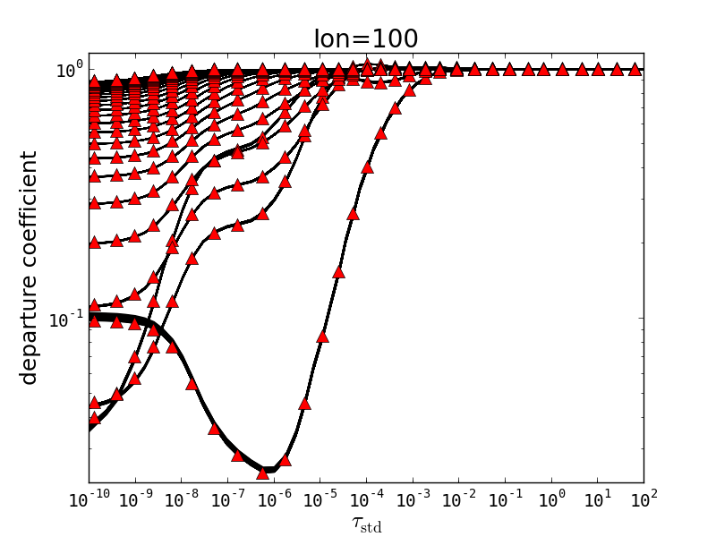
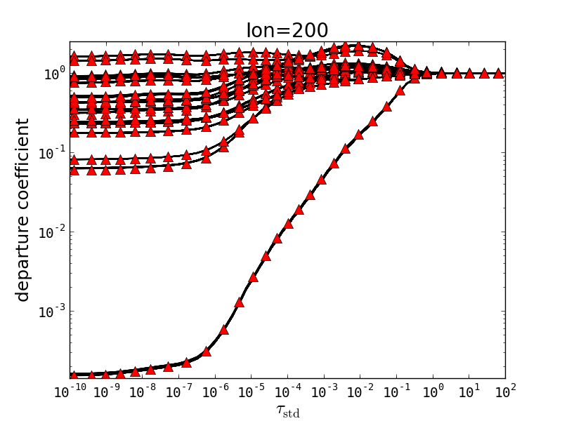
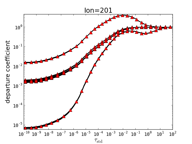
Figure 1: For our first test with NLTE treatment of H I and He I–II, the departure coefficients $b_{i}$, are shown. The red symbols show the results of the 1D calculation whereas the black lines show the results of the 3D calculation for all voxels.

In Fig. 1 we display the departure coefficients $b_{i}\equiv n_{i}/n_{i}^{*}$ for H I, He I and He II. The (red) symbols show the results of the 1D calculation whereas the black lines show the results of the 3D calculation for all voxels. The spread of the black lines is due to the limited solid angle resolution used in the 3D test run (see Hauschildt & Baron 2010, for details). The agreement is excellent, only for the outermost layers with $\tau_{1.2\mu}<10^{-5}$ there are small differences between the 1D and 3D departure coefficients for the lower levels. These differences could be caused by the small $(\theta,\phi)$ voxel resolution of the 3D test (the $r$ resolution is nearly identical to the 1D model, see Baron et al. 2012, for a similar effect).

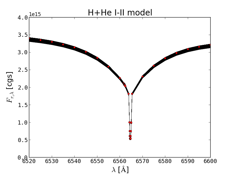
Figure 4: For our first test with NLTE treatment of H I and He I–II the spectral region near $H_{\alpha}$ is shown. The red lines show the results of the 1D NLTE calculation whereas the black lines show the maximum and minimum of the radial component of the flux vector over all outermost voxels from the 3D calculation. The spread in the 3D model is due to the finite numerical resolution, see paper VI.

The spectra in the regions around the Lyman and Balmer jumps and $H_{\alpha}$ are compared in Figs. 2 – 4, where the red symbols are again the 1D fluxes and the black lines are the radial components of the flux vectors at the surface voxels of the 3D model (the wavelength resolution was taken directly from the NLTE iterations). The spectra are nearly identical, the “bandwidth” in the 3D spectra is again the resolution effect discussed in Hauschildt & Baron (2010). In the wings of the Balmer lines, the resolution spread in the flux results in differences of about 5% to the the 1D model. To reduce the spread by 1/2, we estimate based on the results of Paper VI that about 4 times more solid angle points are needed, which is no problem for full production calculations. Note that only the NLTE lines and continua and LTE background continua are included in the modeling (to save time), no LTE background lines are considered.

The second test uses the same basic setup as discussed above, but includes a full NLTE treatment for H and He and the first 3 ionization stages of C, N, O, and Mg. In detail, the setup is identical for H and He and we use C I (230 levels), C II (85 levels), C III (79 levels), N I(254 levels), N II (152 levels), N III(87 levels), O I (146 levels), O II (171 levels), O III (137 levels), Mg I (179 levels), Mg II (74 levels), and Mg III (90 levels), for a total of 21 ions, 1749 levels, and 15478 line transitions. As before we use an identical setup for the 1D comparison calculations.

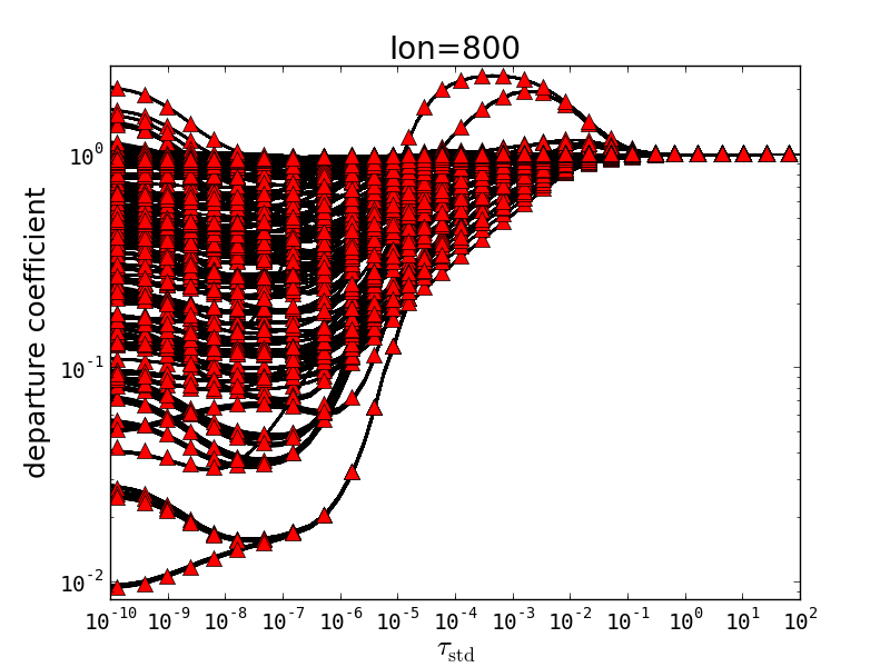
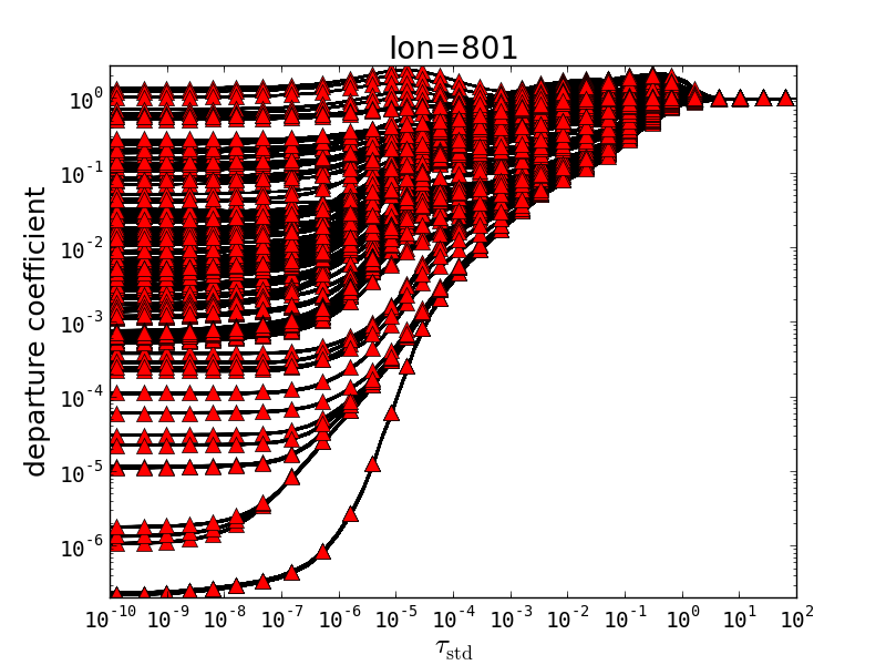
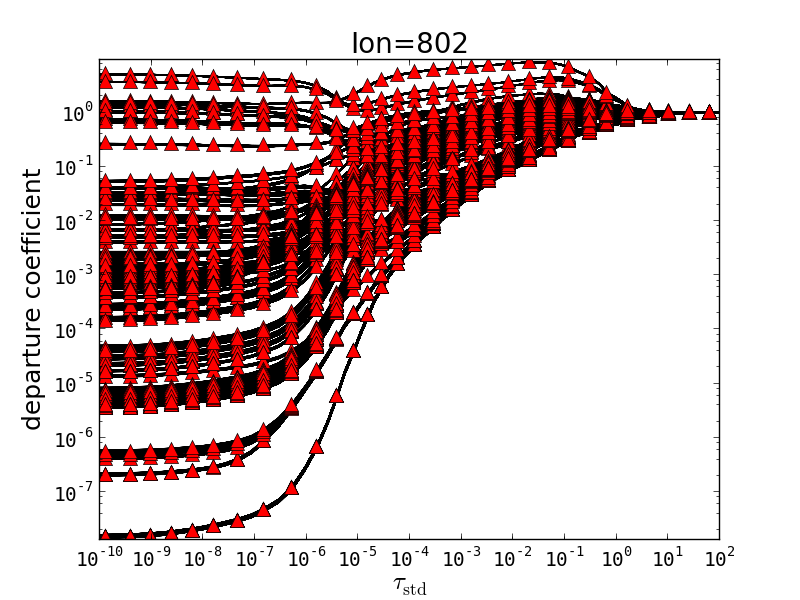
Figure 7: For our second test case with NLTE treatment of H I, He I–II, C I–III, N I—III, O I—III, and Mg I—III the departure coefficients, $b_{i}$, for O I—III are shown. The red symbols show the results of the 1D calculation whereas the black lines show the results of the 3D calculation for all voxels.

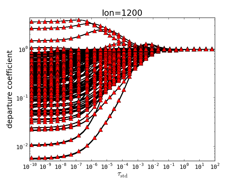
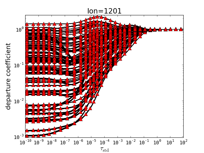
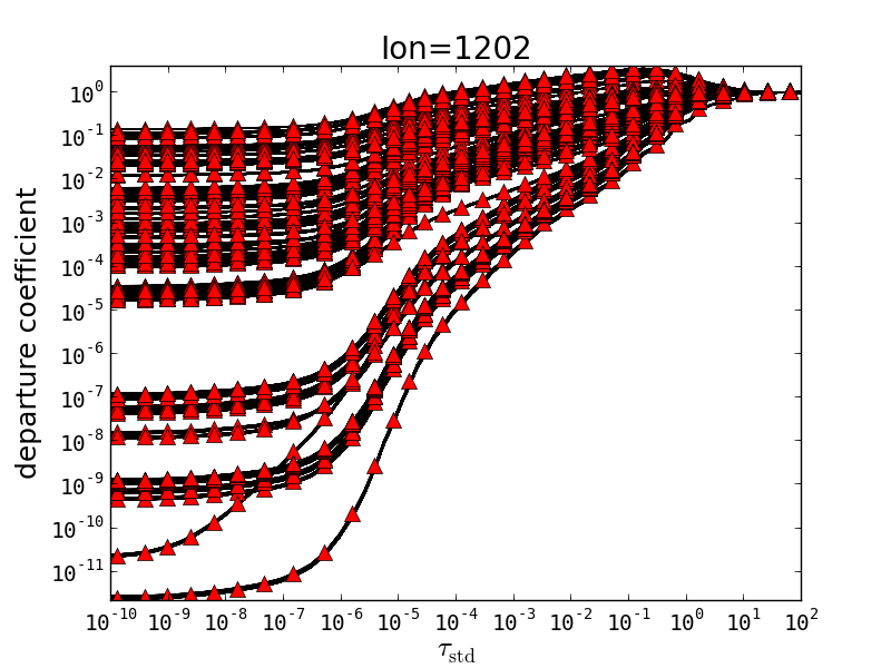
Figure 8: For our second test case with NLTE treatment of H I, He I–II, C I–III, N I—III, O I—III, and Mg I—III the departure coefficients, $b_{i}$, for Mg I—III are shown. The red symbols show the results of the 1D calculation whereas the black lines show the results of the 3D calculation for all voxels.

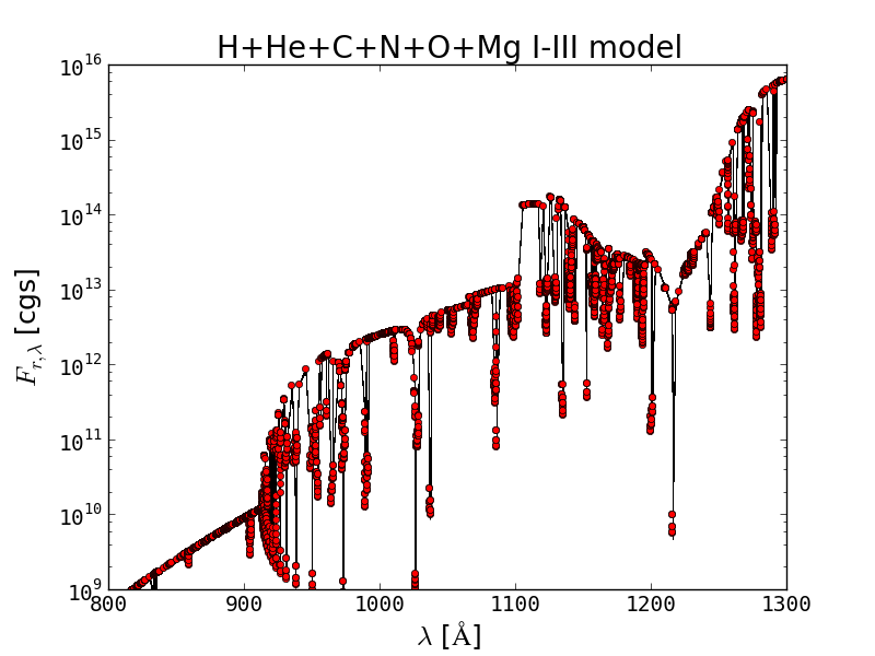
Figure 9: For our second test case with NLTE treatment of H I, He I–II, C I–III, N I—III, O I—III, and Mg I—III the spectral region near the Lyman break is shown. The red lines show the results of the 1D NLTE calculation whereas the black lines show the maximum and minimum of the radial component of the flux vector over all outermost voxels from the 3D calculation. The spread in the 3D model is due to the finite numerical resolution, see paper VI.

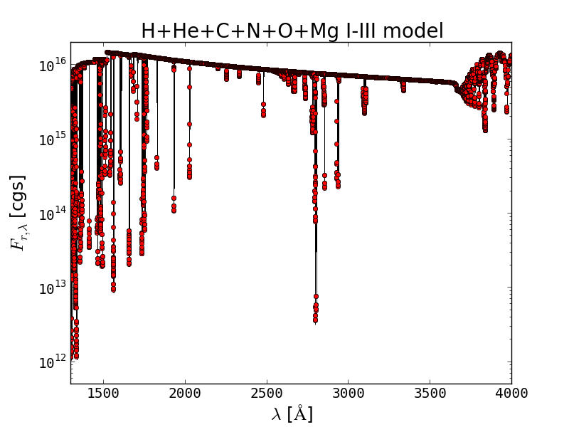
Figure 10: For our second test case with NLTE treatment of H I, He I–II, C I–III, N I—III, O I—III, and Mg I—III the spectral region in the near UV is shown. The red lines show the results of the 1D NLTE calculation whereas the black lines show the maximum and minimum of the radial component of the flux vector over all outermost voxels from the 3D calculation. The spread in the 3D model is due to the finite numerical resolution, see paper VI.

Some of the results for the departure coefficients are shown in examples in Figs. 5 – 8. The comparison to the equivalent 1D model is of the same quality as in the simpler test case shown above. The plots show only every other point from the 1D model to reduce clutter. Even complex behavior in the departure coefficients is well reproduced in the 3D model. The deviations from the 1D model are smaller than the width of the bands produced by the numerical resolution of the solid angle grid (see Hauschildt & Baron 2010). Similar results hold for the spectra, shown for two examples in Figs. 9 and 10.

This test model has about 111,000 wavelength points (about 10 times more than the small test case) and requires about 706GB to store the full spectral data (mean intensities and flux vectors for all voxels and wavelengths for detailed analysis), storing just the outer spectrum (flux vectors) for plotting requires about 5GB, the departure coefficients and occupation number densities require about 2.7GB storage for all voxels. The larger test was run on a Cray XE30 supercomputer using 49248 MPI processes (2052 nodes) using about 970MB RAM per process and 2680 seconds wallclock per iteration. For comparison, the 1D equivalent model uses about 43s per iteration with 48 MPI processes on the same machine.

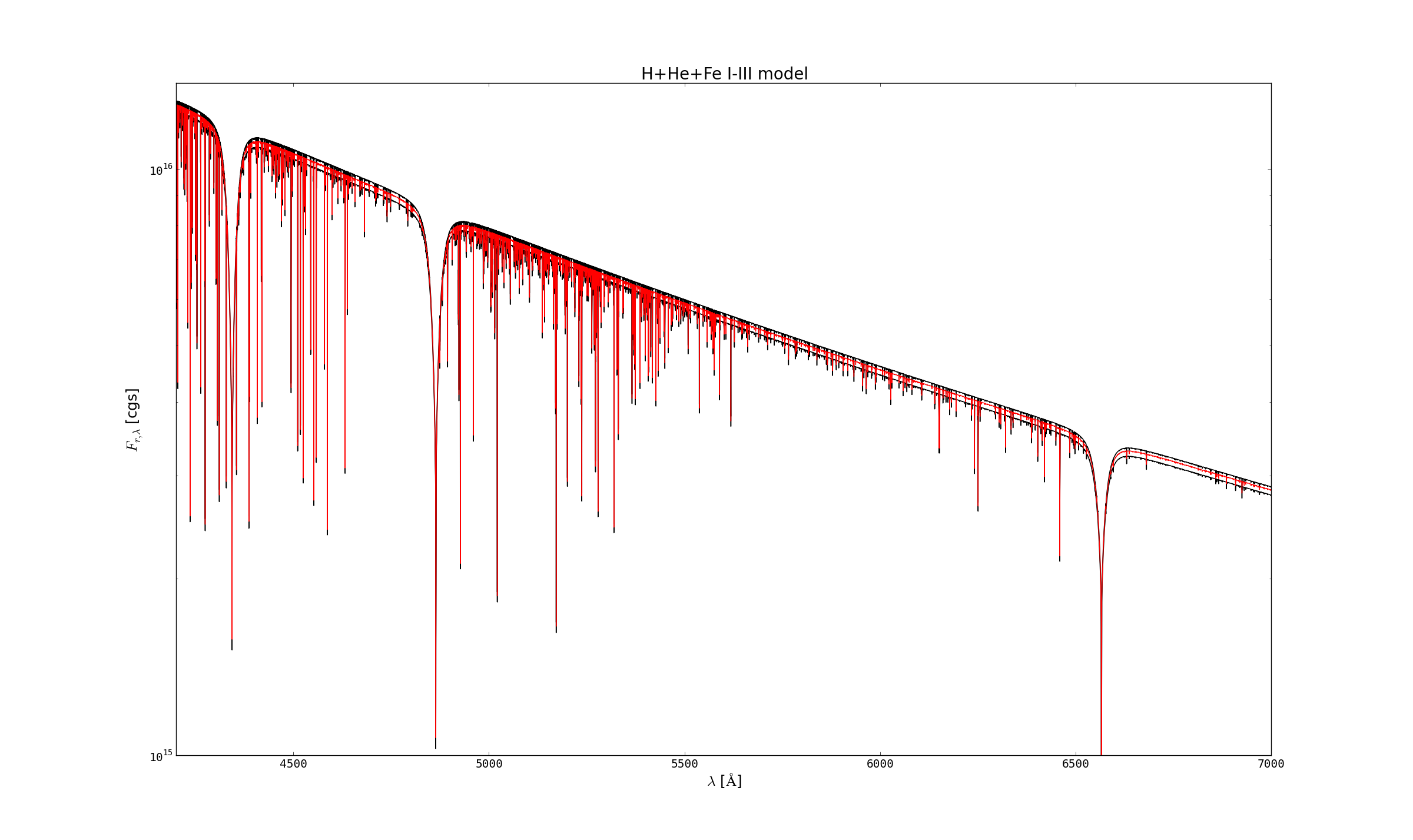
Figure 13: For our third test case with NLTE treatment of H I, He I–II, and Fe I–III, the spectral region in the optical is shown. The red lines show the results of the 1D NLTE calculation whereas the black lines show the maximum and minimum of the radial component of the flux vector over all outermost voxels from the 3D calculation. The spread in the 3D model is due to the finite numerical resolution, see paper VI.

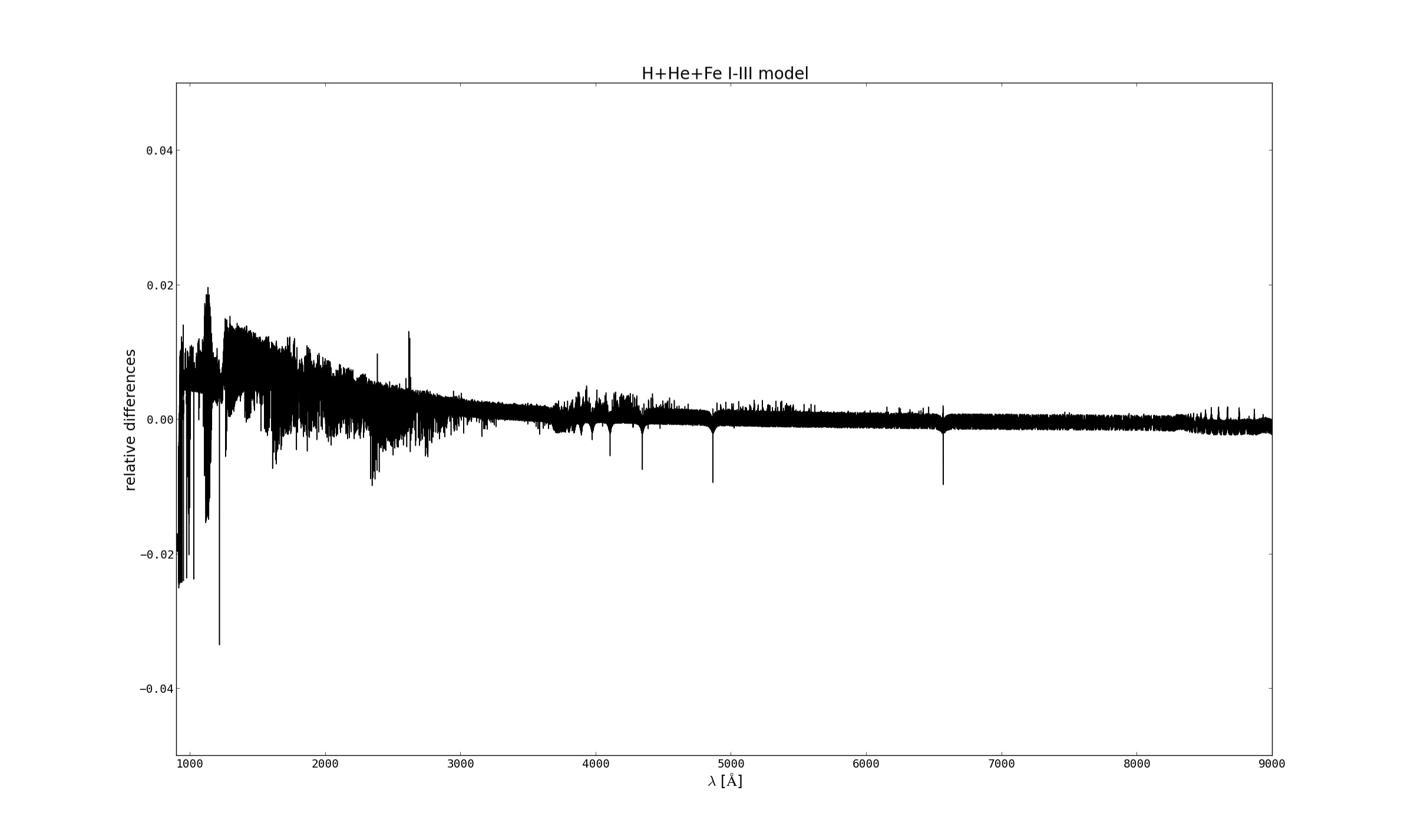
Figure 14: Relative differences between the fluxes of the 1D comparison model and the arithmetic average over all outermost voxels of the $r$ component of the flux vector of the 3D calculation for the test case with NLTE treatment of H I, He I–II, and Fe I–III.

In order to test a very large model (in present day terms), we repeated the calculation for a setup with H, He and Fe I-III in NLTE. In this case, the Fe model atoms are significantly larger than the model atoms used before. With the same setup for H and He as above, we have now Fe I (902 levels, 24395 lines ) Fe II (894 levels, 22453 lines) and Fe III (555 levels, 9867 lines), for a total of 57232 individual lines and 2410 b-f transitions. The number of levels per Fe ion is so large, what we plot only every 10th level in Fig. 11 for clarity. The agreement between 1D and 3D models is again excellent, the differences are below the variances caused by the resolution of the 3D model. In Figs. 12 – 13 we show two wavelength ranges comparing 1D (red lines) and 3D spectra. The plot shows the maximum and minimum over all outermost voxels, the spread is due to the finite numerical resolution, (see Hauschildt & Baron 2010, Paper VI). The comparison in these cases is also very good. We show as an example in Fig. 14 the relative differences between the 1D comparison model and the arithmetic mean of the $r$ components of the 3D flux vectors over all outermost voxels. With the exception of a few wavelengths, the differences are below 2%, which is very good given the limits of the resolution in solid angle. The spectrum of this model contains close to 0.5 million wavelength points, the storage requirements for the 3D spectral data (all voxels, complete information for imaging including flux vectors) is about 2.6TB.

5 Summary and Conclusions

In this paper we discussed a method to solve 3D multi-level radiative transfer problems with detailed model atoms. The method is a direct extension of the well-tested method we are using for 1D model atmosphere calculations. We have implemented this NLTE/3D module for PHOENIX/3D and discussed a small to very large test calculations for code testing and validation. The results show that the method performs in 3D exactly as the 1D equivalent. The NLTE problem in 3D poses significant demands on the computing resources, therefore we designed the module for distributed memory parallel processing (MPI) and to use domain decomposition methods to reduce the memory requirements per process. With this, it is technically possible to even solve 3D NLTE problems for complex ions, e.g., the iron group, if large supercomputers are used.

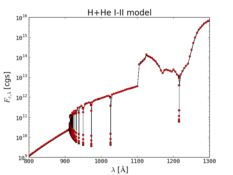
Figure 2: For our first test with NLTE treatment of H I and He I–II the spectral region near the Lyman break is shown. The red lines show the results of the 1D NLTE calculation whereas the black lines show the maximum and minimum of the radial component of the flux vector over all outermost voxels from the 3D calculation. The spread in the 3D model is due to the finite numerical resolution, see (Hauschildt & Baron 2010, paper VI).

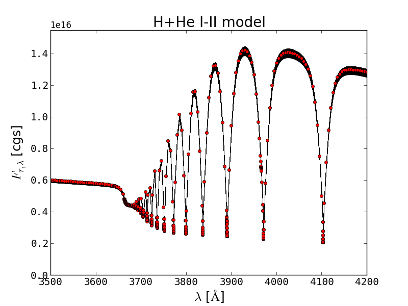
Figure 3: For our first test with NLTE treatment of H I and He I–II the spectral region near the Balmer jump is shown. The red lines show the results of the 1D NLTE calculation whereas the black lines show the maximum and minimum of the radial component of the flux vector over all outermost voxels from the 3D calculation. The spread in the 3D model is due to the finite numerical resolution, see paper VI.

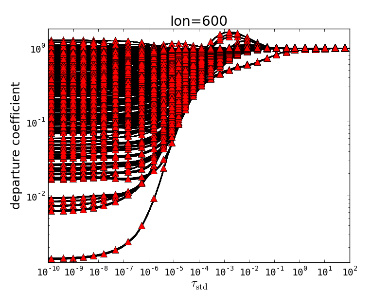
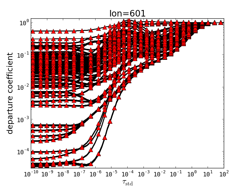
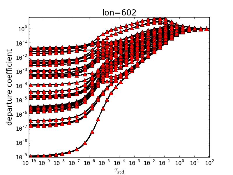
Figure 5: For our second test case with NLTE treatment of H I, He I–II, C I–III, N I—III, O I—III, and Mg I—III the departure coefficients, $b_{i}$, for C I—III are shown. The red symbols show the results of the 1D calculation whereas the black lines show the results of the 3D calculation for all voxels.

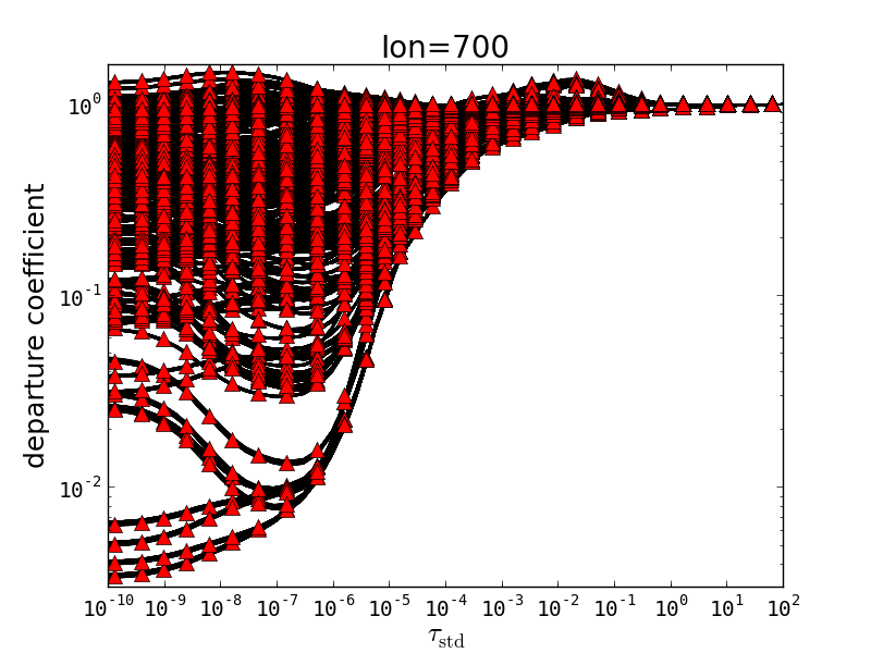
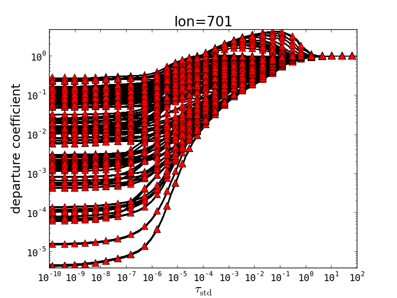
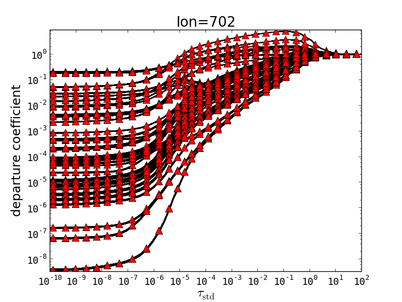
Figure 6: For our second test case with NLTE treatment of H I, He I–II, C I–III, N I—III, O I—III, and Mg I—III the departure coefficients, $b_{i}$, for N I—III are shown. The red symbols show the results of the 1D calculation whereas the black lines show the results of the 3D calculation for all voxels.

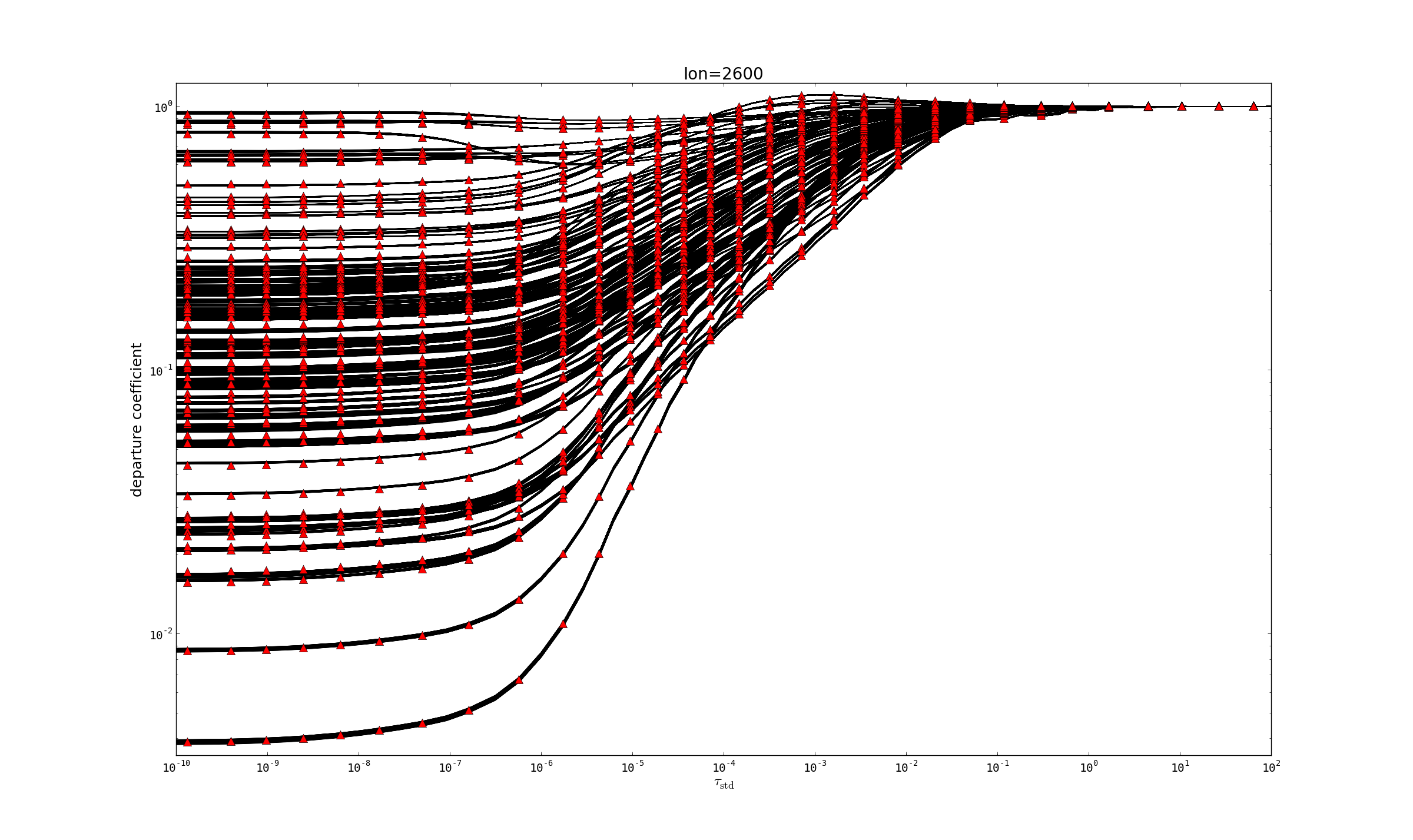
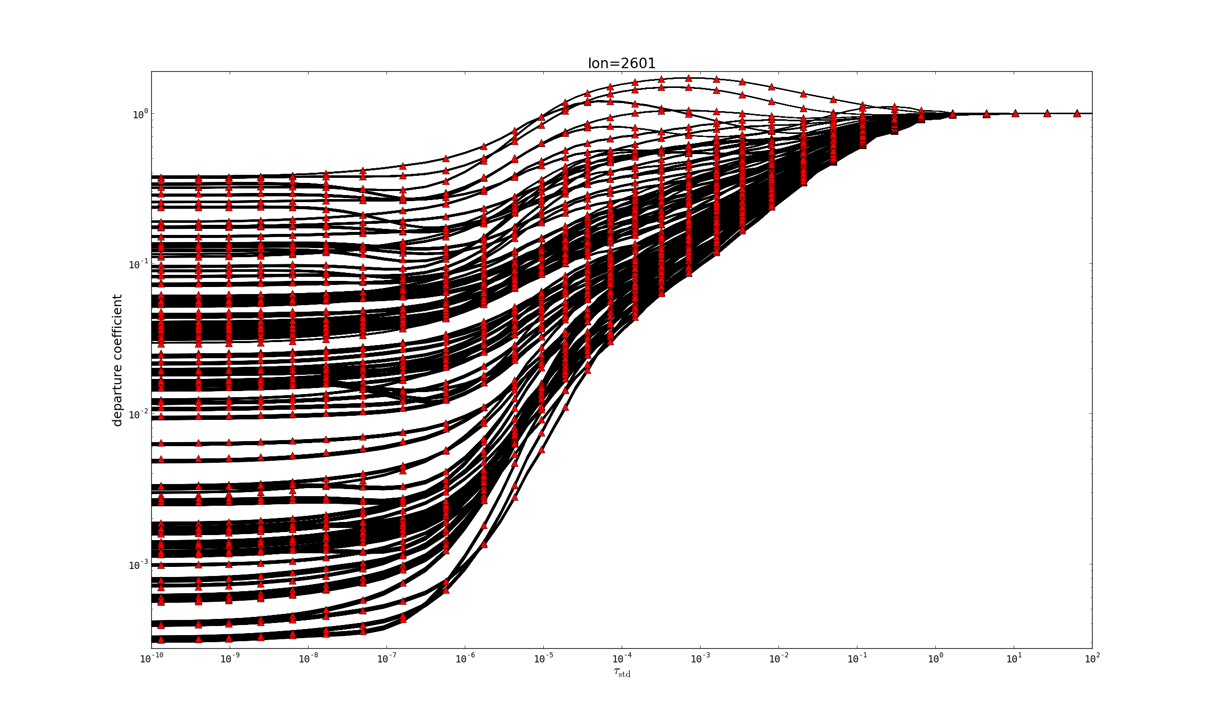
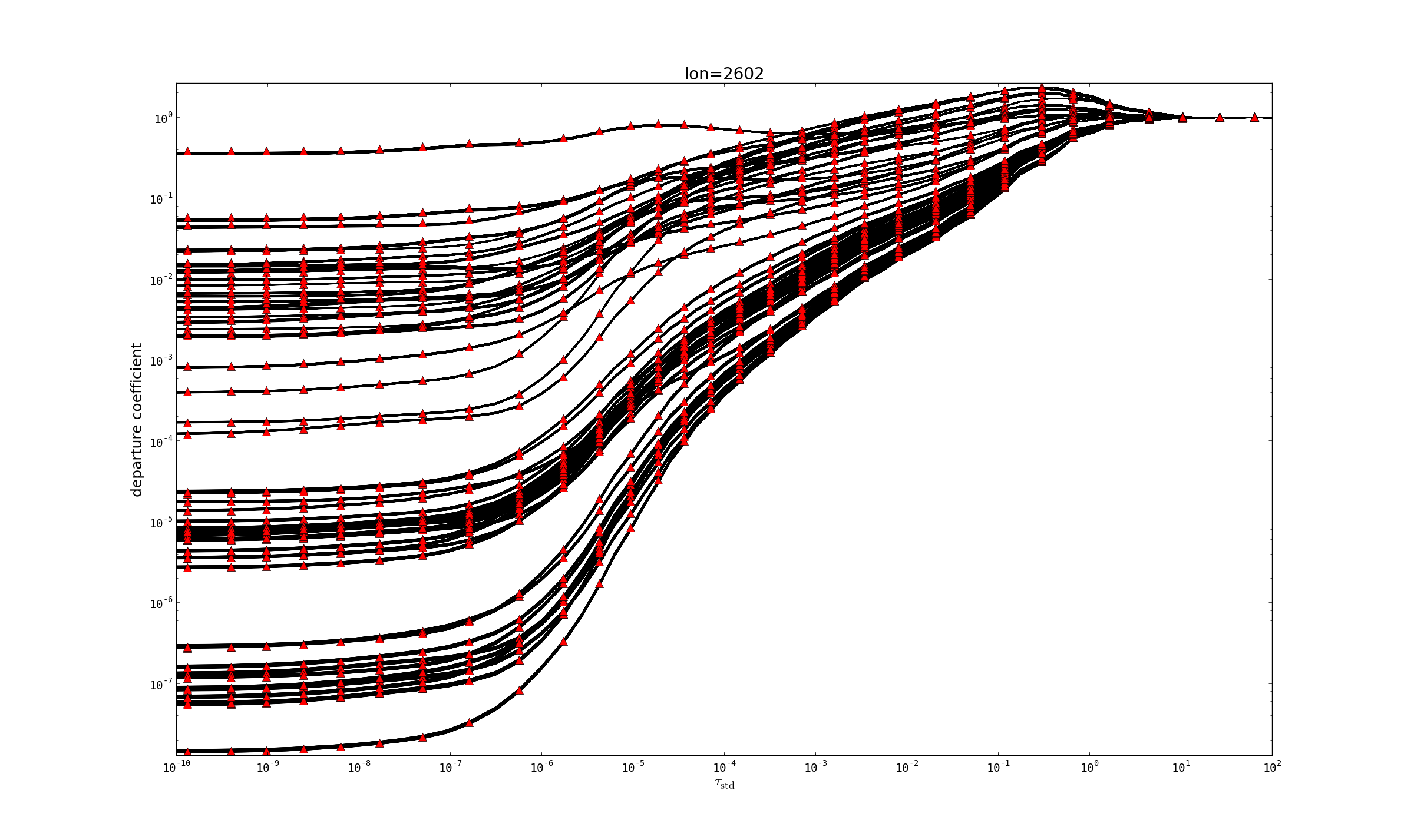
Figure 11: For our third test case with NLTE treatment of H I, He I–II, and Fe I–III, the departure coefficients, $b_{i}$, for Fe I—III are shown. For clarity, we plot only every 10th level. The red symbols show the results of the 1D calculation whereas the black lines show the results of the 3D calculation for all voxels.

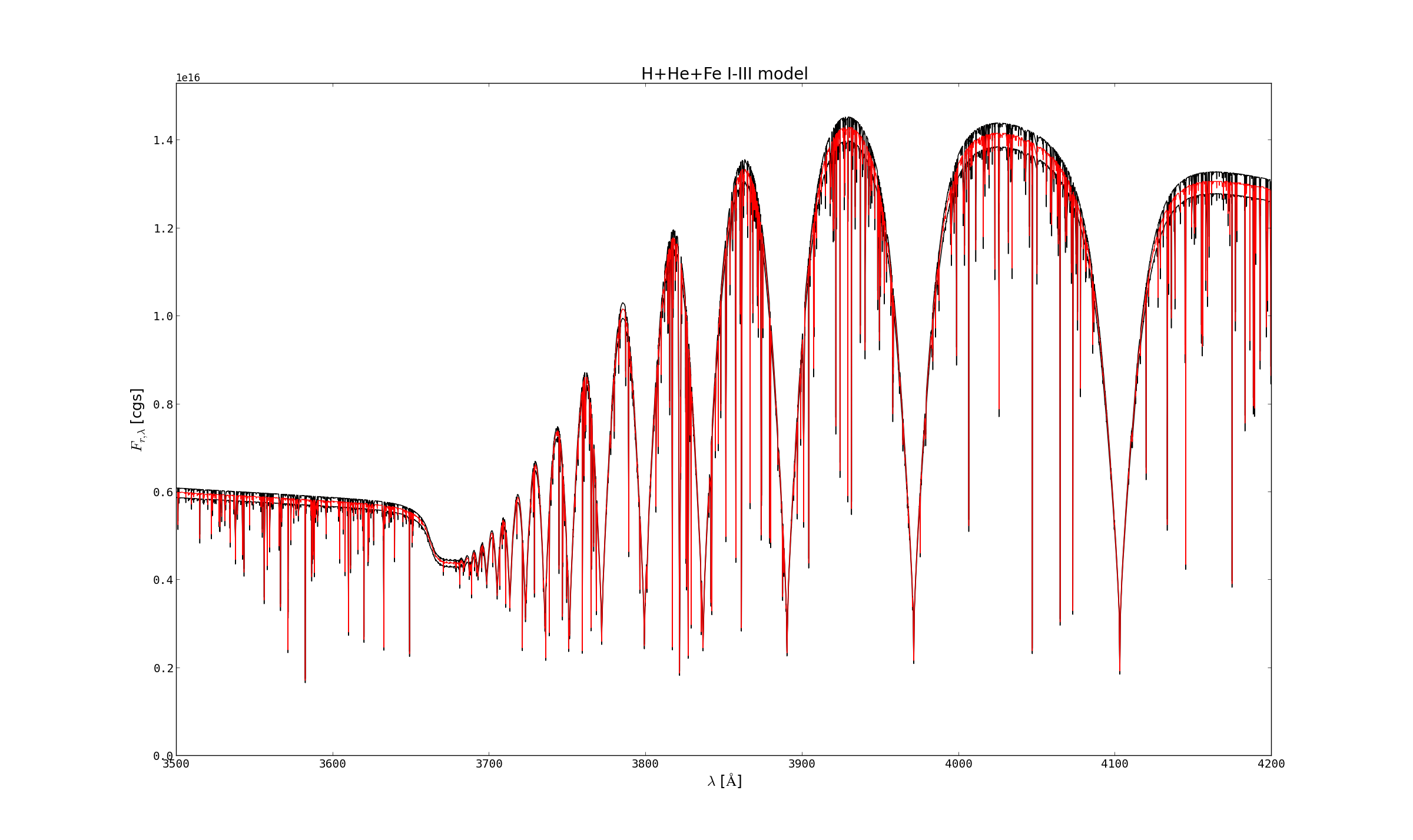
Figure 12: For our third test case with NLTE treatment of H I, He I–II, and Fe I–III, the spectral region near the Balmer jump is shown. The red lines show the results of the 1D NLTE calculation whereas the black lines show the maximum and minimum of the radial component of the flux vector over all outermost voxels from the 3D calculation. The spread in the 3D model is due to the finite numerical resolution, see paper VI.