Generalized Dimers and their Stokes-variable Dynamics

Abstract

In the present work, we generalize the setting of dimers with potential gain and loss which have been extensively considered recently in $\mathcal{PT}$-symmetric contexts. We consider a pair of waveguides which are evanescently coupled but may also be actively coupled and may possess onsite gain and loss, as well as (possibly non-uniform) nonlinearity. We identify (and where appropriate review from earlier work) a plethora of interesting dynamical scenaria ranging from the existence of stable and unstable fixed points and integrable dynamics, to the emergence of pitchfork or Hopf bifurcations and the generation of additional fixed points and limit cycles, respectively, as well as the potential deviation of trajectories to infinity. Thus, a catalogue of a large number of possible cases is given and their respective settings physically justified (where appropriate).

I Introduction

Over the past decade and a half, there has been an intense interest in the theme of open systems featuring gain and loss due to numerous developments in the study of $\mathcal{PT}$-symmetric dynamics; see e.g. Bender_review ; special-issues ; review . While the original proposal of such systems was given in the context of quantum mechanical (non-Hermitian, yet still potentially bearing real eigenvalues) Hamiltonians, relevant applications sprang in a number of diverse areas of physical interest. In particular, the analogy between the Schrödinger equation in quantum mechanics and the paraxial propagation equation in optics led to such proposals in optics Muga ; PT_periodic which were subsequently realized in a series of experiments experiment . Additionally, “engineered” $\mathcal{PT}$ symmetric systems also arose in the context of electronic circuits; see the work of tsampikos_recent and also the review of tsampikos_review . Further developments including mechanical systems pt_mech and even whispering-gallery microcavities pt_whisper have recently followed.

The realization of $\mathcal{PT}$ symmetry in optical settings naturally brought forth the question of the implications of nonlinearity in such systems, as nonlinearity is rather ubiquitous in optics Musslimani2008 . This, in turn, led to the exploration of structures such as bright Yang and dark dark ; vortices solitons, two-dimensional generalizations of solitons midya , as well as vortices vortices . Generalizations of one-dimensional dual ; dual2 and two-dimensional Burlak such entities were predicted to exist as stable objects in dual-core couplers (with the gain and loss being present in different cores). In addition, a large number of studies focused on the context of discrete systems in the setting of few sites (so-called oligomers), as well as lattices kot1 ; sukh1 ; kot2 ; grae1 ; grae2 ; pgk ; dmitriev1 ; dmitriev2 ; R30add5 ; R34 ; R44 ; R46 ; baras1 ; baras2 ; konorecent3 ; leykam ; konous ; uwe ; tyugin ; pickton .

The present work is in the spirit of oligomers and more specifically of dimers examined rather exhaustively in recent years both in experiments experiment and in theory kot1 ; sukh1 ; grae1 ; grae2 ; pgk ; R44 ; R46 ; tyugin ; pickton . However, it also fundamentally differs from these works, as it is not in the “standard” (and rather delicate in its necessitated balance of gain and loss) $\mathcal{PT}$-symmetric realm. Instead, we seek to further explore a setting put forth in the recent, fundamental contribution of barasflach , where an active medium with two waveguides, each contributing to the gain of the other is set forth, coupled with the intrinsic loss of each waveguide. While the resulting setting of barasflach is not $\mathcal{PT}$-symmetric, it is demonstrated that it features a robust feedback loop, which, in turn, generates stationary and oscillatory regimes in a wide range of gain-loss parameter values. Additionally, the resulting system as written in the so-called Stokes variables presents an intriguing proximity to the classical Lorenz dynamical system which is a prototype of chaotic dynamics. Indeed, the work of barasflach revealed a sizable region of their two dimensional (gain-loss) parameter space exhibiting chaotic dynamics.

Our aim here is to present a general form of the relevant dimer system inter-twining the characteristics of (a) an active medium, (b) evanescent coupling, (c) intrinsic loss or imposed gain on each waveguide and finally nonlinearity (of possibly even non-uniform type) and to explore the situation for different types of combinations of these characteristics. In each of the cases considered, we explore the Stokes variable formalism and rewrite the dynamical system as a 3 degree-of-freedom setup (effectively removing an overall trivial phase, associated with the U$(1)$ invariance of the dimer). Subsequently, we perform the “local” analysis of the system, identifying its fixed points and their spectral characteristics, as well elucidating the potential bifurcations (pitchforks, Hopfs, etc.). Finally, we complement the theoretical analysis with direct numerical computations which illustrate prototypical dynamics of the respective cases.

The presentation is structured as follows. In section II, we briefly present the general setup associated with our system. In section III, we catalogue the relevant subcases and their theoretical (fixed point, stability and bifurcation) analysis, as well as the associated numerical computations. Finally, in section IV, we summarize our main findings and present a number of conclusions and directions for future work.

II Theoretical Setup

We start by considering in the spirit of barasflach the general dimer system for the evolution of two waveguides with variables $u_{1}(t)$, $u_{2}(t)$ according to:

$$\dot{u}_{1} = (a_{1}+i\sigma)u_{2}+b_{1}u_{1}-iP_{1}|u_{1}|^{2}u_{1},$$ (1)

$$\dot{u}_{2} = (a_{2}+i\sigma)u_{1}+b_{2}u_{2}-iP_{2}|u_{2}|^{2}u_{2}.$$ (2)

Here, $a_{1,2}$ play the role of the active underlying medium, which we will broadly conceive of as not necessarily symmetrically acting on the two waveguides (although the latter is the canonical physical case). Here, for mathematical purposes, we will also expand the realm of considerations to cases with $a_{1}\neq a_{2}$. On the other hand, $\sigma$ plays the role of the evanescent coupling between the waveguides and $b_{1,2}$ is the respective gain and loss imposed individually (or intrinsically) on each waveguide. Finally, $P_{1,2}$ will represent the nonlinearity strength of the cubic Kerr effect. For the latter, again motivated by physical cases of different material properties as e.g. in settings of the form of towers ; martincent , we will not a priori assume equal strength of the nonlinear prefactors.

In the following discussion, we will use the well-established Stokes variables kot1 ; tyugin ; pickton ; barasflach $X=\frac{1}{2}(|u_{1}|^{2}-|u_{2}|^{2})$, $Y=\frac{i}{2}(u_{1}u_{2}^{*}-u_{2}u_{1}^{*})$ and $Z=\frac{1}{2}(u_{1}u_{2}^{*}+u_{2}u_{1}^{*})$. By also rescaling time as $\tilde{t}=2t$, our dynamical equations can be rewritten as follows:

$$\frac{dX}{d\tilde{t}} = \frac{a_{1}-a_{2}}{2}Z-\sigma Y+\frac{1}{2}(b_{1}|u_{1}|^{2}-b_{2}|u_{2}|^{2}),$$ (3)

$$\frac{dY}{d\tilde{t}} = \frac{b_{1}+b_{2}}{2}Y+\sigma X+\frac{1}{2}(P_{1}|u_{1}|^{2}-P_{2}|u_{2}|^{2})Z,$$ (4)

$$\frac{dZ}{d\tilde{t}} = \frac{1}{2}(a_{2}|u_{1}|^{2}+a_{1}|u_{2}|^{2})+\frac{b_{1}+b_{2}}{2}Z-(P_{1}|u_{1}|^{2}-P_{2}|u_{2}|^{2})Y.$$ (5)

We now let $N=\frac{1}{2}(|u_{1}|^{2}+|u_{2}|^{2})$ i.e., the optical power, and thus $X^{2}+Y^{2}+Z^{2}=N^{2}$; notice that given this formula and the definition of $X$ and $N$, we can always express the above equations as a three-dimensional dynamical system. The differential equation for the evolution of $N$ reads:

$$\frac{dN}{d\tilde{t}} = \frac{a_{1}+a_{2}}{2}Z+\frac{1}{2}(b_{1}|u_{1}|^{2}+b_{2}|u_{2}|^{2}).$$ (6)

With conditions $a_{1}+a_{2}=0$ and $b_{1}=b_{2}$, $N$ is exponentially increasing ($b>0$) or decreasing ($b<0$), hence it is straightforward to establish instability $(b>0)$ or stability $(b<0)$ about the origin, which is the only fixed point. Hence we focus more on systems where parameters do not satisfy these conditions.

It is also interesting to note that if we write $u_{1}=\rho_{1}e^{i(\phi+\theta)}$ and $u_{2}=\rho_{2}e^{i\phi}$, then the Stokes Variables can be expressed using $\rho_{1}$, $\rho_{2}$ and $\theta$, i.e., the overall free phase due to the gauge invariance of the model is the dynamical variable that has been eliminated in this system. More specifically, $X=\frac{1}{2}(\rho_{1}^{2}-\rho_{2}^{2})$, $Y=\rho_{1}\rho_{2}\sin\theta$ and $Z=\rho_{1}\rho_{2}\cos\theta$. Based only on these three equations, $Y$ and $Z$ are two similar variables (playing the role of polar coordinates for the pair $(\rho_{1}\rho_{2},\theta)$, while $X$ measures the intensity difference between the waveguides.

Reversing the relevant transformation, $\rho_{1}$ and $\rho_{2}$ and $\theta$ can also be obtained from Stokes Variables: $\theta={\rm arctan}\frac{Y}{Z}$, $\rho_{1}^{2}=\sqrt{X^{2}+Y^{2}+Z^{2}}+X$ and $\rho_{2}^{2}=\sqrt{X^{2}+Y^{2}+Z^{2}}-X$. In what follows, we will solely consider the analysis of the three-dimensional dynamical system in the realm of Stokes Variables, bearing the above transformations and inverse transformations in mind.

III Catalogue of Different Parametric Cases

III.1 $a_{1}=a_{2}=0$

This is the case connecting to the earlier work including in $\mathcal{PT}$-symmetric settings where the medium is not active in that it does not induce a gain or loss related coupling between the waveguides.

III.1.1 $b_{1}=b_{2}=b$

Since $a_{1}=a_{2}=0$ automatically leads to $a_{1}+a_{2}=0$, if we also assume equal gain or loss on two waveguides ($b_{1}=b_{2}=b$), the system is quite straightforward: the origin is the sole fixed point and it is either a stable spiral (for $b<0$) or an unstable spiral (for $b>0$). Also note that the Stokes variable system bears an obvious reflection symmetry if $(x,y)$ is replaced by $(-x,-y)$ (for $P_{1}=P_{2}$) or replacing $(x,y,z)$ by $(-x,-y,-z)$ (for $P_{1}=-P_{2}$).

III.1.2 $b_{1}=-b_{2}=b$, $P_{1}=P_{2}=P$

The system in this case reads:

$$\frac{dX}{d\tilde{t}} = -\sigma Y+bN,$$ (7)

$$\frac{dY}{d\tilde{t}} = \sigma X+PXZ,$$ (8)

$$\frac{dZ}{d\tilde{t}} = -PXY.$$ (9)

In fact, this is the well studied case of the $\mathcal{PT}$-symmetric dimer. For the latter, it is well known that it possesses two conserved quantities $C^{2}=Y^{2}+(Z+\frac{\sigma}{P})^{2}$ and $J=N+\frac{b}{p}\arcsin(\frac{Z+\frac{\sigma}{P}}{C})$, and is hence integrable, possessing also the potential for periodic orbits. The ability of the system depending on the relative values of $b$ and $\sigma$ to settle into periodic orbits or to escape to $\infty$ has been elucidated in a series of recent works  kot1 ; tyugin ; pickton ; barasflach2 .

In this case, the differential equation $\frac{d}{d\tilde{t}}(N)=bX$ does not provide direct dynamical information but solely an a priori bound to the growth of the system tyugin . To better understand the dynamics, we reshape Eqs. (8)-(9) into a harmonic oscillator form pelinovsky using the variable $s(\tilde{t})=\int_{0}^{\tilde{t}}X(t^{\prime})dt^{\prime}$. Then the solutions of $Y$ and $Z$ are:

$$Y(\tilde{t}) = C_{1}\cos(Ps(\tilde{t}))+C_{2}\sin(Ps(\tilde{t})),$$ (10)

$$Z(\tilde{t}) = -\frac{\sigma}{P}+C_{2}\cos(Ps(\tilde{t}))-C_{1}\sin(Ps(\tilde{t})),$$ (11)

where $C_{1}$ and $C_{2}$ are constants, determined by the initial conditions. These imply not only that $Y$ and $Z$ are always bounded, but also that $Y^{2}+(Z+\frac{\sigma}{P})^{2}$ is constant over time. Thus, the dynamical system is actually two dimensional and any trajectory is constrained on the surface of a cylinder. By exploring the dynamics of $|u_{1}|^{2}$ and $|u_{2}|^{2}$, we can show that the density can become unbounded if the initial values are suitably chosen. Besides, an example of explicit unbounded solution has been reported in barasflach2 .

The fixed points in this case are $(0,0,0)$ and $(0,\frac{b}{\sigma}N,\pm\frac{\sqrt{\sigma^{2}-b^{2}}}{\sigma}N)$ for any non-negative number $N$. Since $N=\sqrt{X^{2}+Y^{2}+Z^{2}}$ is not continuously differentiable at $(0,0,0)$, interestingly, it is not straightforward to examine the Jacobian matrix of the fixed point of the origin (at the level of our Stokes variable equations). Instead, in such a case it is advisable to return to the original dynamical system revealing that for $b^{2}<\sigma^{2}$ the origin is a stable fixed point (center), while the converse is true for $b^{2}>\sigma^{2}$ (saddle). The two additional families of fixed points correspond to the symmetric and anti-symmetric (for $b=0$) states of the Hamiltonian analog of the dimer which indeed collide and disappear in a saddle-center bifurcation at $\sigma^{2}=b^{2}$, as is well-known pgk for such  $\mathcal{PT}$-symmetric dimers.

More generally, in this setting for $b^{2}<\sigma^{2}$, as is well-known, the trajectories may be bounded (periodic) or unbounded kot1 ; pgk ; tyugin ; pickton ; barasflach2 , while for $b^{2}>\sigma^{2}$, they will be generically unbounded.

III.1.3 $b_{1}=-b_{2}=b$, $P_{1}=-P_{2}=P$

This is an interesting case that to the best of our knowledge has not been explored previously. Here the linear part of the system is $\mathcal{PT}$-symmetric, while the nonlinear part is not. The dynamical equations for the Stokes variables in this case read:

$$\frac{dX}{d\tilde{t}} = -\sigma Y+bN,$$ (12)

$$\frac{dY}{d\tilde{t}} = \sigma X+PNZ,$$ (13)

$$\frac{dZ}{d\tilde{t}} = -PNY.$$ (14)

Once again, the evolution of the power does not lead to unambiguous results since $\frac{d}{d\tilde{t}}(N)=bX$, but solely to an a priori bound for its maximal growth rate since $X\leq N$ (and hence the maximal growth rate of the exponential growth of $N$ is $b$).

The origin is the sole fixed point in this case. The linearization around it is again not feasible at the level of Eq. (14) but can instead be realized at the level of Eq. (2) suggesting that the origin is a center for $b^{2}<\sigma^{2}$ and a saddle point for $b^{2}>\sigma^{2}$. It is worth noting that the center here is no longer a center for a pure two-dimensional system, as was the case in the previous subsection and it, thus, does not necessarily imply the existence of a periodic orbit. A complementary perspective of this from the point of view of the Stokes variables is that when $b^{2}>\sigma^{2}$, $|bN|>|\sigma Y|$ so that $X$ is always increasing or decreasing. Notice that the same inequality can be used to infer the indefinite growth at the broken $\mathcal{PT}$-symmetry regime (past the $\mathcal{PT}$-phase transition) in the context of Eq. (9).

By constructing the special function $L=NX-\frac{\sigma}{P}Z$, we can show $\frac{d}{d\tilde{t}}L=b(N^{2}+X^{2})$ so that $L$ is monotonic for nonzero $b$. This confirms that the origin is the only fixed point. Moreover, the system cannot bear any periodic orbits. If it did, integrating $L$ along the orbit would never give zero, which is a contradiction to the integrated equation. Therefore, even though this case has exactly the same linearization around the origin as the previous case A.2, the dynamics there can be quite different, as shown in Fig. 1.

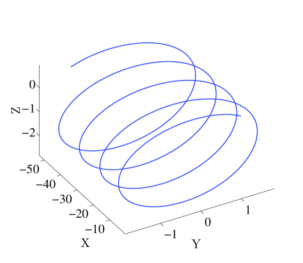
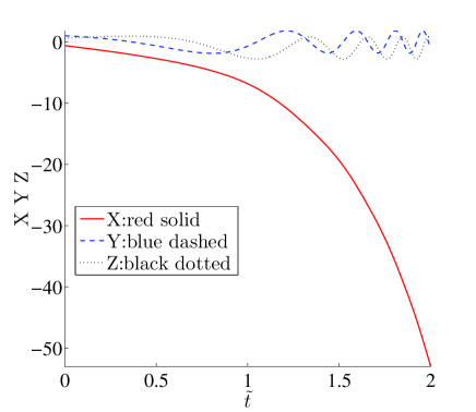
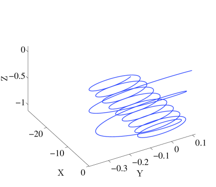
Figure 1: The top panels are related to the case $b^{2}>\sigma^{2}$ with $b=-2$, $\sigma=1$, $P=-1$, starting near the origin $(0,0,0)$ in the Stokes variables and ending up with $X\to-\infty$. The bottom panels are for the case of $\sigma^{2}>b^{2}$ and $b=-0.5$, $\sigma=1$, $P=-1$. Here the trajectory still escapes to infinity, instead of forming a closed orbit. The left panels both here and in subsequent plots show the evolution in the three-dimensional phase space of $X$, $Y$ and $Z$, while the right panels show the evolution of each of these Stokes variables over time.

III.2 $a_{1}=a_{2}=a$

We now turn to the case of the active medium, assuming initially, as is done also in barasflach (and as is most physically relevant), an equal effect of the active medium on the two waveguides.

III.2.1 $b_{1}=b_{2}=b$, $P_{1}=P_{2}=P$

In this case, the system in the Stokes variables reads:

$$\frac{dX}{d\tilde{t}} = -\sigma Y+bX,$$ (15)

$$\frac{dY}{d\tilde{t}} = bY+\sigma X+PXZ,$$ (16)

$$\frac{dZ}{d\tilde{t}} = aN+bZ-PXY.$$ (17)

In this case, the equations remain unchanged if $(x,y)$ is replaced by $(-x,-y)$, while the evolution of $N$ yields $\frac{d}{d\tilde{t}}(N)=bN+aZ$. So when $b^{2}>a^{2}$, $N$ grows to infinity or decays all the way to zero as time $\tilde{t}$ evolves. For $b^{2}<a^{2}$, we go back to the original system (2) and consider two invariant manifolds. If $u_{1}=u_{2}=u$, the system can be reduced as $\dot{u}=(a+b+i\sigma)u-iP|u|^{2}u$ and we can show $\frac{d|u|^{2}}{dt}=2(a+b)|u|^{2}$. If $u_{1}=-u_{2}=u$, the system reads: $\dot{u}=(-a+b-i\sigma)u-iP|u|^{2}u$. The dynamical equation of $|u|^{2}$ becomes $\frac{d|u|^{2}}{dt}=2(-a+b)|u|^{2}$. Since $|a|>|b|$, one of these two manifolds features exponentially growing solutions while the other only contains exponentially decaying solutions. To be more specific, we can actually give explicit forms for these bounded and unbounded solutions:

$$u_{1}=u_{2}=Ce^{(a+b)t+i\phi(t)},~{}~{}~{}\phi(t)=\sigma t-\frac{P}{2(a+b)}e^{2(a+b)t}+\phi_{0}$$ (18)

and

$$u_{1}=-u_{2}=Ce^{(b-a)t+i\phi(t)},~{}~{}~{}\phi(t)=-\sigma t-\frac{P}{2(b-a)}e^{2(b-a)t}+\phi_{0},$$ (19)

where $C$ and $\phi_{0}$ are constants determined by initial values. The instability of the unbounded solution has been discussed in  barasflach2 .

On the other hand, the local analysis yields an interesting cascade of bifurcations. In particular, $(0,0,0)$ is always a fixed point; the eigenvalues of Eq. (2) when linearizing around the origin are $-a+b-i\sigma$ and $a+b+i\sigma$. When $a^{2}>b^{2}$, this fixed point becomes unstable, doing so through a pitchfork bifurcation resulting in the emergence of two new fixed points, namely $F^{+}=(\sqrt{\frac{(a^{2}-b^{2})(b^{2}+\sigma^{2})}{P^{2}b^{2}}},\frac{b}{\sigma}\sqrt{\frac{(a^{2}-b^{2})(b^{2}+\sigma^{2})}{P^{2}b^{2}}},-\frac{b^{2}+\sigma^{2}}{P\sigma})$ and $F^{-}=(-\sqrt{\frac{(a^{2}-b^{2})(b^{2}+\sigma^{2})}{P^{2}b^{2}}},-\frac{b}{\sigma}\sqrt{\frac{(a^{2}-b^{2})(b^{2}+\sigma^{2})}{P^{2}b^{2}}},-\frac{b^{2}+\sigma^{2}}{P\sigma})$.

The characteristic equation for these fixed points $F^{+}$(or $F^{-}$) is $\lambda^{3}-2b\lambda^{2}+\frac{(a^{2}-b^{2})\sigma^{2}}{b^{2}}\lambda-\frac{(a^{2}-b^{2})(b^{2}+\sigma^{2})}{b}=0$. When $b^{2}=\sigma^{2}$, the Jacobian matrix at $F^{+}$(or $F^{-}$) has a real eigenvalue $2b$ and two pure imaginary eigenvalues $\lambda^{2}=-\frac{\sigma^{2}(a^{2}-b^{2})}{b^{2}}=b^{2}-a^{2}$. As a result, at this point this system becomes subject to a Hopf bifurcation giving birth to the existence of limit cycles.

Subsequent period doublings of the limit cycles yield progressively a route to chaotic dynamics, as was systematically analyzed for this case in barasflach . Hence, in this case the dynamics of the system is very rich. In fact, it transitions from asymptoting to $(0,0,0)$ to asymptoting to a stable steady state (through a pitchfork) [these two scenaria are illustrated in Fig. 2] and then from asymptoting to a periodic orbit eventually to a fully chaotic dynamics [these two scenaria are shown in Fig. 3]. These findings corroborate the analysis of the pioneering study in this generalized context of active media of barasflach .

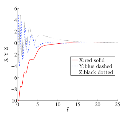
Figure 2: The top panels show the case (for the active system) of $a^{2}<b^{2}$ with $a=0.2$, $b=-0.4$, $\sigma=1$, $P=-1$, resulting into approach to the origin $(0,0,0)$ in the Stokes variables. The bottom panels are for the supercritical case of $a^{2}>b^{2}$ with $b^{2}<\sigma^{2}$ and $a=1$, $b=-0.4$, $\sigma=1$, $P=-1$. Here the stable steady state $F^{+}$ is approached (as the origin has become unstable).

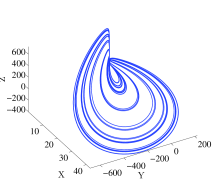
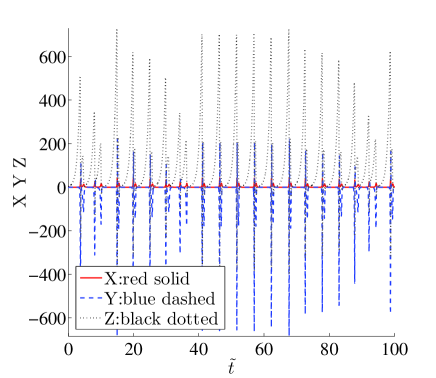
Figure 3: The top two panels show the case where $a^{2}>b^{2}$ with $b^{2}>\sigma^{2}$: $a=2$, $b=-1.5$, $\sigma=1$, $P=-1$. Here the orbit locks into a limit cycle (as we are past the Hopf bifurcation point destabilizing $F^{\pm}$). Finally, the bottom two panels show the case of substantially larger values of $b^{2}$ with $a^{2}>b^{2}$ and $b^{2}>\sigma^{2}$ for $a=9$, $b=-7.6$, $\sigma=1$, $P=-1$. Here the response of the system is chaotic.

III.2.2 $b_{1}=b_{2}=b$, $P_{1}=-P_{2}=P$

We now turn to another case which constitutes an interesting variant of the case studied in barasflach . In particular, again bearing in mind the case of waveguides of different materials with different nonlinear properties, we consider the case where $P_{1}=-P_{2}=P$, i.e., one waveguide with a focusing and one with a self-defocusing nonlinearity.

The system in this case is of the form:

$$\frac{dX}{d\tilde{t}} = -\sigma Y+bX,$$ (20)

$$\frac{dY}{d\tilde{t}} = bY+\sigma X+PNZ,$$ (21)

$$\frac{dZ}{d\tilde{t}} = aN+bZ-PNY.$$ (22)

The stability analysis of the origin in this case is the same as in case B.1. Moreover, when $(a^{2}-b^{2})>0$, there is also $F=(\frac{\sigma(a^{2}-b^{2})}{Pab},\frac{(a^{2}-b^{2})}{Pa},-\frac{b}{a}\sqrt{\frac{(a^{2}-b^{2})(b^{2}+\sigma^{2})}{P^{2}b^{2}}})$. The linearization around this fixed point leads to the polynomial equation (for the eigenvalues): $\lambda^{3}-2b\lambda^{2}+\lambda(\frac{a^{2}(\sigma^{2}+b^{2})}{b^{2}})+\frac{(b^{2}+\sigma^{2})(b^{2}-a^{2})}{b}=0$. If the equation has three real roots, they are always negative ($b<0$) or positive ($b>0$). If two of the roots are complex conjugates and one is real, it can be easily checked that the real root always has the same sign as $b$. By expressing $(\sigma^{2}+b^{2})$ as a function of three roots and using the fact it is positive, we find here the real part of the complex roots also shares the sign of $b$. Thus we find that $a^{2}>b^{2}$ changes the origin to a saddle and admits the emergence of a stable (if $b<0$) or unstable (if $b>0$) fixed point in $F$.

These stability conclusions are mirrored in the dynamics of Fig. 4. For $a^{2}<b^{2}$ (top panels), we observe that the evolution is driven to the origin, while for $a^{2}>b^{2}$ (bottom panels), the dynamics leads to the stable steady state $F$ (for our case of $b<0$). Note that if we change $b$ from negative to positive, the evolution will do something opposite to the above figures, spiraling out from the fixed point (such as the origin in the top panels or $F$ in the bottom panels) towards infinity.

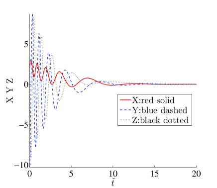
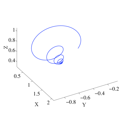
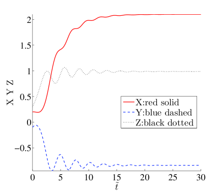
Figure 4: Top panels: case of $a^{2}<b^{2}$ with $a=0.5$, $b=-1.5$, $\sigma=1$, $P=1$ leading to decay towards the origin. Bottom panels: case of $a^{2}>b^{2}$ with $a=0.5$, $b=-0.2$, $\sigma=1$, $P=1$. Here the origin is unstable and the evolution leads to the stable nontrivial fixed point $F$.

III.2.3 $b_{1}=-b_{2}=b$, $P_{1}=P_{2}=P$

We now turn to a case slightly different from that of barasflach , yet still physically realizable. In particular, the intrinsic gain-loss pattern of the waveguides involves gain in one, and loss in the other (as it does in the $\mathcal{PT}$-symmetric setting), yet the active medium (and the nonlinearity) uniformly affect both.

The system in this case reads:

$$\frac{dX}{d\tilde{t}} = -\sigma Y+bN,$$ (23)

$$\frac{dY}{d\tilde{t}} = \sigma X+PXZ,$$ (24)

$$\frac{dZ}{d\tilde{t}} = aN-PXY.$$ (25)

In this case, it is not straightforward to infer dynamical features from the evolution of $N^{2}$ according to $\frac{d}{d\tilde{t}}(N^{2})=2bNX+2aNZ$. Hence, we turn to the stability of fixed points. $(0,0,0)$ is always a fixed point and its eigenvalues in this case acquire a complicated form in Eq. (2) being given by $\pm\sqrt{a^{2}+b^{2}-\sigma^{2}+2ia\sigma}$, implying the origin is a fixed point of saddle type.

On the other hand, when $b^{2}>\sigma^{2}$, $|bN|>|\sigma Y|$ so that $X$ is always increasing or decreasing. When $\sigma^{2}>b^{2}$, there is an additional fixed point of the form $F=(\frac{a\sigma}{bP},{\rm sign}(b\sigma)\sqrt{\frac{\sigma^{2}(a^{2}+b^{2})}{P^{2}(\sigma^{2}-b^{2})}},-\frac{\sigma}{P})$. The characteristic equation of the Jacobian matrix at $F$ yields

$$\lambda^{3}-\lambda\left(\frac{b^{4}+a^{2}b^{2}-a^{2}\sigma^{2}}{b^{2}}\right)-\frac{a\sigma}{b^{2}P}\sqrt{P^{2}b^{2}(\sigma^{2}-b^{2})(a^{2}+b^{2})}=0.$$ (26)

Since the coefficient of second order term is zero, we know immediately that at least one of the eigenvalues should have a positive real part. Hence we conclude that the trajectory near $F$ is unbounded in one or two directions given by the corresponding eigenvectors and this fixed point is never stable.

Despite the existence of such an additional fixed point, we thus find in this case that the generic instability of $F$, as well as that of the origin lead the dynamics to feature an evolution of $|X|\to\infty$ or of $|Y|,|Z|\to\infty$. This is clearly demonstrated in Fig. 5, showcasing the relevant dynamics both for the case of $\sigma^{2}<b^{2}$ (top panels), as well as in that of $\sigma^{2}>b^{2}$ (bottom panels).

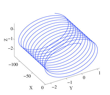
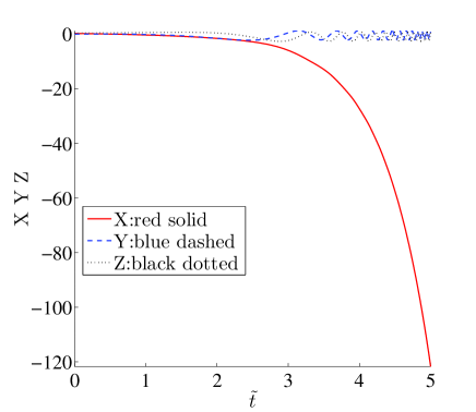
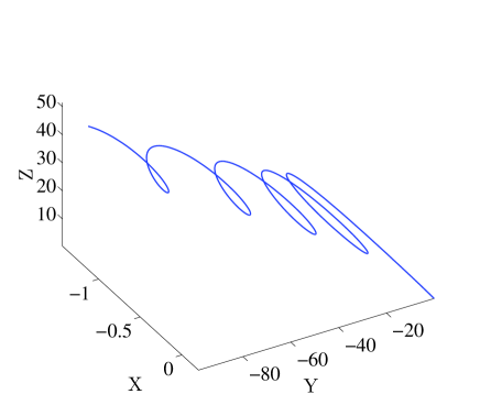
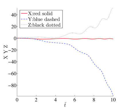
Figure 5: The top panel contains the case of $\sigma^{2}<b^{2}$ with $a=0.5$, $b=-1.5$, $\sigma=1$, $P=1$. The origin is the sole (yet unstable) fixed point here with the dynamics leading $X\to-\infty$, while $Y$ and $Z$ will circle around $Y=-0.5,Z=-1$. On the other hand, the bottom panels are for the case with $\sigma^{2}>b^{2}$ with $a=1$, $b=-0.9$, $\sigma=1$, $P=1$. Here $Y,Z$ tend to $\pm\infty$, while $X$ stays bounded. The latter implies that the amplitudes of both waveguides tend to $\infty$.

III.2.4 $b_{1}=-b_{2}=b$, $P_{1}=-P_{2}=P$

Finally, we consider the case where features of cases B.2 and B.3 are combined, namely while the active medium is present, the waveguides are made of different materials (featuring one with focusing and the other with self-defocusing nonlinearity), while the intrinsic gain/loss structure supports one waveguide with gain and features loss in the other.

The system in this case reads:

$$\frac{dX}{d\tilde{t}} = -\sigma Y+bN,$$ (27)

$$\frac{dY}{d\tilde{t}} = \sigma X+PNZ,$$ (28)

$$\frac{dZ}{d\tilde{t}} = aN-PNY.$$ (29)

The stability analysis of the origin is similar to the case B.3.

In addition, when $\sigma^{2}>b^{2}$ and $\frac{\sigma a}{Pb}>0$, there are also $F^{+}=(\frac{a^{2}}{Pb}\sqrt{\frac{(\sigma^{2}-b^{2})}{(a^{2}+b^{2})}},\frac{a}{P},-\frac{a}{P}\sqrt{\frac{(\sigma^{2}-b^{2})}{(a^{2}+b^{2})}})$ and
$F^{-}=(-\frac{a^{2}}{Pb}\sqrt{\frac{(\sigma^{2}-b^{2})}{(a^{2}+b^{2})}},\frac{a}{P},\frac{a}{P}\sqrt{\frac{(\sigma^{2}-b^{2})}{(a^{2}+b^{2})}})$. The characteristic equation of Jacobian matrix at $F^{+}$(or $F^{-}$) is $\lambda^{3}+\lambda\frac{a^{2}\sigma^{2}+b^{2}\sigma^{2}-b^{4}}{b^{2}}+\mp\frac{a\sigma\sqrt{(\sigma^{2}-b^{2})(a^{2}+b^{2})}}{b}=0$. By similar analysis as in case B.3, we know at either $F^{+}$ or $F^{-}$ one eigenvalue has positive real part and the other two come with negative real parts, while the real parts of eigenvalues at the other fixed point have exactly opposite signs, namely, two positive and one negative.

What is found in the dynamics, as well as from the detailed consideration of different parameter values is that when $\sigma^{2}<b^{2}$, the instability of the origin appears to generically lead to divergence (whereby $X$ tends to $\infty$). On the other hand, while the same behavior is possible also for $\sigma^{2}>b^{2}$ (see the bottom panels of Fig. 6 for a relevant case example), in the latter case it appears to also be possible to observe periodic (closed cycle in the phase plane) behavior around the fixed points. To be more specific, if we initialize somewhere between the fixed points $F^{+}$ and $F^{-}$, the system will just keep circling between $F^{+}$ and $F^{-}$, as illustrated in the two examples of Fig. 7. However, a slightly different initialization may lead to wandering around these fixed points for a while but eventually escaping to infinity (see the top panels in Fig. 6). Notably, the result of the evolution in these cases appears to be sensitively dependent on the precise form of the initial condition. Finally, choosing the initial position far from these fixed points leads to a rapid growth of $|X|$ towards infinity.

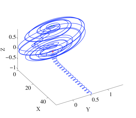
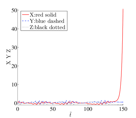
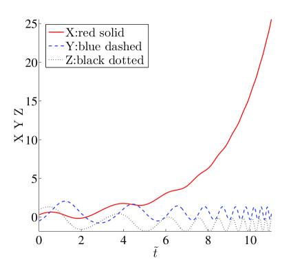
Figure 6: Here, we only show (two examples of) the case with $\sigma^{2}>b^{2}$. In the top panels, $a=0.5$, $b=0.5$, $\sigma=1$, $P=1$, periodic-orbit-looking dynamics can eventually escape to infinity becoming unbounded. For the bottom, if we move the initial condition even further, divergence shows up in the dynamics in a short time (red circle: $F^{+}$; blue cross: the origin; green square: $F^{-}$).

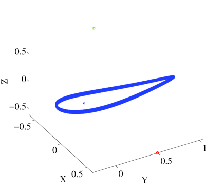
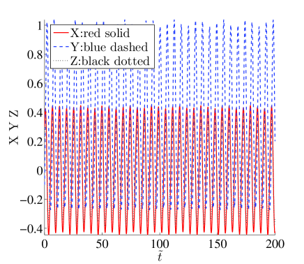
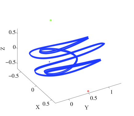
Figure 7: Here we use same parameters as in Fig. 6 but different initial conditions. In the top panels, we can observe here the existence of closed cycles in the $(X,Y,Z)$ plane that appear to correspond to limit cycles in the dynamics. In the bottom panels, if we change the initial position a bit, closed orbits can still be obtained but they may look different (red circle: $F^{+}$; blue cross: the origin; green square: $F^{-}$).

III.3 $a_{1}=-a_{2}=a$

We now turn to a less physically relevant but still mathematically interesting case, where the underlying active medium leads to opposite effects between the two waveguides. That is, it provides cross-coupling gain for one, while it leads to corresponding loss for the other. In the following discussion, we show that this setup makes the system closely resemble the case $a=0$, which is a special case example of the setup of this section.

III.3.1 $b_{1}=b_{2}=b$

The system in this case features equal intrinsic gain (or loss) between the waveguides. As Eq. (6) suggests, we have $\frac{dN}{d\tilde{t}}=bN$ in this sub-case. Similar to case A.1, here the origin is the only possible fixed point of the system and it is either a sink ($b<0$) or a source ($b>0$).

III.3.2 $b_{1}=-b_{2}=b$, $P_{1}=P_{2}=P$

We now turn to additional cases, such as in this section the one where the intrinsic gain/loss pattern is anti-symmetric i.e., $b_{1}=-b_{2}$. Remarkably this case is $\mathcal{PT}$ symmetric in its own right.

The system in the Stokes variables within this case reads:

$$\frac{dX}{d\tilde{t}} = aZ-\sigma Y+bN,$$ (30)

$$\frac{dY}{d\tilde{t}} = \sigma X+PXZ,$$ (31)

$$\frac{dZ}{d\tilde{t}} = -aX-PXY.$$ (32)

As a direct observation, for $b^{2}>a^{2}+\sigma^{2}$, in the $\mathcal{PT}$-symmetry broken regime (see also the discussion below), $|X|$ will increase or decrease monotonically.

Since subsection A.2 describes a special case of the current case, it should not surprise us that techniques used in subsection A.2 can be applied here. In fact, we can again write $Y$ and $Z$ into harmonic oscillator equations:

$$Y(\tilde{t}) = -\frac{a}{P}+C_{1}\cos(Ps(\tilde{t}))+C_{2}\sin(Ps(\tilde{t})),$$ (33)

$$Z(\tilde{t}) = -\frac{\sigma}{P}+C_{2}\cos(Ps(\tilde{t}))-C_{1}\sin(Ps(\tilde{t})).$$ (34)

where $C_{1}$ and $C_{2}$ are two constants related to the initial conditions. So $Y$ and $Z$ are always on a circle centered at $(-\frac{a}{P},-\frac{\sigma}{P})$ and $|u_{1}u_{2}|$ is bounded for all time $\tilde{t}$. Again, if we choose initial values of $u_{1}$ and $u_{2}$ carefully, either $|u_{1}|^{2}$ or $|u_{2}|^{2}$ will blow up to infinity, while the other will decay towards zero.

We find here that the origin is always a fixed point of the system, with the eigenvalues being $\pm\sqrt{b^{2}-a^{2}-\sigma^{2}}$, hence the presence of the active medium extends the region of $\mathcal{PT}$ symmetry in comparison to the well-known case of $a=0$. When $b^{2}>a^{2}+\sigma^{2}$ the origin is a saddle point. When $b^{2}<a^{2}+\sigma^{2}$, the origin becomes a center and fixed points $(0,\frac{b\sigma+a\sqrt{a^{2}+\sigma^{2}-b^{2}}}{\sigma^{2}+a^{2}}N,\frac{-ba+\sigma\sqrt{a^{2}+\sigma^{2}-b^{2}}}{\sigma^{2}+a^{2}}N)$, $(0,\frac{b\sigma-a\sqrt{a^{2}+\sigma^{2}-b^{2}}}{\sigma^{2}+a^{2}}N,\frac{-ba-\sigma\sqrt{a^{2}+\sigma^{2}-b^{2}}}{\sigma^{2}+a^{2}}N)$ (with $N$ nonnegative) arise. Their Jacobian matrices can be directly calculated as having eigenvalues $\lambda(\lambda^{2}-(b^{2}-a^{2}-\sigma^{2}\mp\sqrt{a^{2}+\sigma^{2}-b^{2}}PN))=0$.

As an alternative approach, we introduce cylindrical coordinates in order to obtain a clearer picture of the dynamical system. Let $Y=-\frac{a}{P}+\rho\cos{\theta}$ and $Z=-\frac{\sigma}{P}+\rho\sin{\theta}$, then we obtain:

$$\frac{d\rho}{d\tilde{t}} = 0,$$ (35)

$$\frac{d\theta}{d\tilde{t}} = -PX,$$ (36)

$$\frac{dX}{d\tilde{t}} = a\rho\sin{(\theta)}-\sigma\rho\cos{(\theta)}+b\sqrt{(-\frac{a}{P}+\rho\cos{\theta})^{2}+(-\frac{\sigma}{P}+\rho\sin{\theta})^{2}}.$$ (37)

Since $\frac{dN}{d\tilde{t}}=bX=-\frac{b}{P}\frac{d\theta}{d\tilde{t}}$, we can express $N$ using $\theta$ as $N=-\frac{b}{P}\theta+C$ where $C=N(0)+\frac{b}{P}\theta(0)$. Hence Eqn. (37) can be rewritten as:

$$\frac{dX}{d\tilde{t}}=a\rho\sin{(\theta)}-\sigma\rho\cos{(\theta)}-\frac{b^{2}}{P}\theta+bC.$$ (38)

Note that the above equations are valid except at the origin or when $\rho=0$. When $\rho=0$, the system is as simple as a straight line $Y=-\frac{a}{P},Z=-\frac{\sigma}{P}$ and $X$ moves all the way to $\infty$ ($b>0$) or $-\infty$ ($b<0$).

For other situations, once $\rho$ and $C$ are determined by the initial conditions, fixed points of the two-dimensional system satisfy:

$$X=0,~{}~{}~{}a\rho\sin{(\theta)}-\sigma\rho\cos{(\theta)}-\frac{b^{2}}{P}\theta+bC=0.$$ (39)

and corresponding eigenvalues are given by:

$$\lambda^{2}=b^{2}-P\rho(a\cos{(\theta)}+\sigma\sin{(\theta)}).$$ (40)

Inspired by forms of the dynamical equations of $X$ and $\theta$ and work related to the case $a=0$ barasflach2 , we state that there is an effective energy conservation law for a classical particle fully describing the system:

$$\frac{1}{2}\left(\frac{dq}{d\tilde{t}}\right)^{2}+V(q)=E,$$ (41)

with displacement $q=\theta-\frac{P}{b}C$, potential $V(q)=-\frac{b}{2}q^{2}-aP\rho\cos{(q+\frac{P}{b}C)}-\sigma P\rho\sin{(q+\frac{P}{b}C)}$ and energy $E=\frac{1}{2}P^{2}\rho^{2}-\frac{1}{2}a^{2}-\frac{1}{2}\sigma^{2}$. Exploring the dynamics and phase portrait of this classical system can help us explain our original system, and yields results quite similar to the case A.2. Again, the origin and case $\rho=0$ are excluded from Eqn. (41).

The number of fixed points on the cylinder varies as the radius $\rho$ changes, as it is clearly seen from the expressions of fixed points including $N$. When the radius $\rho$ is small such that $\rho<|\frac{b}{P}|$, there are no fixed points on the cylinder (except the origin as a saddle with $\rho=\sqrt{\frac{a^{2}+\sigma^{2}}{P^{2}}}<|\frac{b}{P}|$) and all trajectories will become unbounded. As $\rho$ grows beyond $|\frac{b}{P}|$, two additional fixed points arise on the cylindrical surface. It can be checked via their eigenvalues that one of them is center and the other is a saddle. Thus some trajectories can form periodic orbits around the center and others simply run away to infinity along the cylinder.

III.3.3 $b_{1}=-b_{2}=b$, $P_{1}=-P_{2}=P$

Finally, we examine this case, which is interesting in its own right, as it is $\mathcal{PT}$-symmetric at the linear level, while the nonlinearity breaks the symmetry. The system in this case is:

$$\frac{dX}{d\tilde{t}} = aZ-\sigma Y+bN,$$ (42)

$$\frac{dY}{d\tilde{t}} = \sigma X+PNZ,$$ (43)

$$\frac{dZ}{d\tilde{t}} = -aX-PNY.$$ (44)

As usual, in this case too, the origin is always a fixed point and actually it is the only one. Its stability is determined by the same conditions as in case C.2. Furthermore, when $b^{2}>a^{2}+\sigma^{2}$, $\frac{dX}{d\tilde{t}}$ will never change its sign over time, as is shown in the previous case.

As a general version of case A.3, we can similarly construct a special function $L_{1}=NX-\frac{a}{P}Y-\frac{\sigma}{P}Z$. Then its dynamical equation reads $\frac{dL_{1}}{d\tilde{t}}=b(N^{2}+X^{2})$ so that $L_{1}$ always increases or decreases. This property of $L_{1}$ disproves (similarly to the argument discussed in the case A.3) the potential existence of any periodic orbits in the system.

For the dynamics in Stokes variables, we find that it repeats some features reported in case A.3. When $b^{2}>a^{2}+\sigma^{2}$, as shown from the dynamical equation of $X$, $X$ clearly goes to $\infty$ ($b>0$) or $-\infty$ ($b<0$); see top panels in Fig. 8. Even when $b^{2}<a^{2}+\sigma^{2}$, the evolution still leads to unboundedness, especially for $X$, as captured in the bottom panels of Fig. 8.

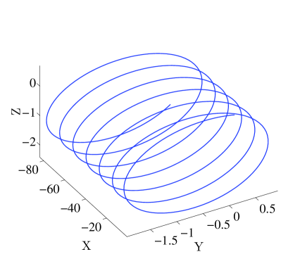
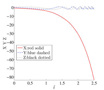
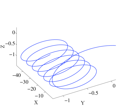
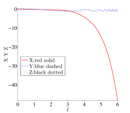
Figure 8: The top panels are under the condition $b^{2}>a^{2}+\sigma^{2}$ with $a=0.5$, $b=-2$, $\sigma=1$, $P=-1$, showing the origin $(0,0,0)$ is not stable here since $X\to-\infty$. The bottom panels are for the case of $b^{2}<a^{2}+\sigma^{2}$ and $a=0.7$, $b=-1.2$, $\sigma=1$, $P=-1$. Again, the evolution will lead to the blowing up of $|X|$ instead of circling around the origin as in case C.2.

IV Conclusions and Future Challenges

In the present work, we have explored a series of generalized examples of the dimer system. Our considerations involved a number of special cases such as the “standard” $\mathcal{PT}$ symmetric dimer kot1 ; sukh1 ; pgk ; R44 ; R46 ; tyugin ; pickton , the actively coupled optical waveguides of barasflach for particular values of the parameters, as well as numerous cases that have not been previously considered, such as a $\mathcal{PT}$ symmetric variation of the actively coupled system or another variant which is $\mathcal{PT}$ symmetric at the linear level but nonlinearity destroys the symmetry. Generally, we introduced and examined the possibility of not only having nonlinearly uniform waveguides but also waveguides constructed of different materials and hence with different (here considered as opposite) Kerr coefficients.

In general, this broad class of systems led to a wide range of interesting behaviors and bifurcation phenomena. In addition to analyzing the stability of the origin, we identified pitchfork bifurcations that gave rise to new fixed points, and Hopf bifurcations that led to the emergence (e.g. in the active medium case) of limit cycles. Moreover, chaotic dynamics was revealed in some of the cases. Furthermore, various diagnostics including the use of Stokes variables and of their dynamical systems’ analysis were brought to bear in order to characterize the dynamics of the different subcases.

Naturally, there are numerous veins for the extension of the present study. On the one hand, for one dimensional systems, it is quite relevant to extend these dimer settings to other oligomer cases, including examples of trimers pgk ; kaiser , quadrimers pgk ; konorecent3 and appreciate how the phenomenology observed herein is extended in this larger number of degrees of freedom cases. On the other hand, extending the relevant phenomenology to higher dimensions and plaquette type configurations as in the case of uwe would be another natural possibility in its own right. Such possibilities are currently under active consideration and will be reported in future publications.

References

- (1) C. M. Bender, Rep. Prog. Phys. 70, 947 (2007).
- (2) See special issues: H. Geyer, D. Heiss, and M. Znojil, Eds., J. Phys. A: Math. Gen. 39, Special Issue Dedicated to the Physics of Non-Hermitian Operators (PHHQP IV) (University of Stellenbosch, South Africa, 2005) (2006); A. Fring, H. Jones, and M. Znojil, Eds., J. Math. Phys. A: Math Theor. 41, Papers Dedicated to the Subject of the 6th International Workshop on Pseudo-Hermitian Hamiltonians in Quantum Physics (PHHQPVI) (City University London, UK, 2007) (2008); C.M. Bender, A. Fring, U. Günther, and H. Jones, Eds., Special Issue: Quantum Physics with non-Hermitian Operators, J. Math. Phys. A: Math Theor. 41, No. 44 (2012).
- (3) K. G. Makris, R. El-Ganainy, D. N. Christodoulides, and Z. H. Musslimani, PT symmetric periodic optical potentials, Int. J. Theor. Phys. 50, 1019 (2011).
- (4) A. Ruschhaupt, F. Delgado, and J. G. Muga, J. Phys. A: Math. Gen. 38, L171 (2005).
- (5) K. G. Makris, R. El-Ganainy, D. N. Christodoulides, and Z. H. Musslimani, Phys. Rev. Lett. 100, 103904 (2008); S. Klaiman, U. Günther, and N. Moiseyev, ibid. 101, 080402 (2008); O. Bendix, R. Fleischmann, T. Kottos, and B. Shapiro, ibid. 103, 030402 (2009); S. Longhi, ibid. 103, 123601 (2009); Phys. Rev. B 80, 235102 (2009); Phys. Rev. A 81, 022102 (2010).
- (6) A. Guo, G. J. Salamo, D. Duchesne, R. Morandotti, M. Volatier-Ravat, V. Aimez, G. A. Siviloglou, and D. N. Christodoulides, Phys. Rev. Lett. 103, 093902 (2009); C. E. Rüter, K. G. Makris, R. El-Ganainy, D. N. Christodoulides, M. Segev, and D. Kip, Nature Phys. 6, 192 (2010); A. Regensburger, C. Bersch, M.-A. Miri, G. Onishchukov, D. N. Christodoulides, and U. Peschel, Nature 488, 167 (2012).
- (7) J. Schindler, A. Li, M.C. Zheng, F.M. Ellis, and T. Kottos, Phys. Rev. A 84, 040101 (2011).
- (8) J. Schindler, Z. Lin, J. M. Lee, H. Ramezani, F. M. Ellis, and T. Kottos, J. Phys. A: Math. Theor. 45, 444029 (2012).
- (9) C. M. Bender, B. Berntson, D. Parker, and E. Samuel Am. J. Phys. 81, 173 (2013).
- (10) B. Peng, S.K. Özdemir, F. Lei, F. Monifi, M. Gianfreda, G.L. Long, S. Fan, F. Nori, C.M. Bender and L. Yang, arXiv: 1308.4564.
- (11) Z. H. Musslimani, K. G. Makris, R. El-Ganainy, and D. N. Christodoulides, Phys. Rev. Lett. 100, 030402 (2008); Z. Lin, H. Ramezani, T. Eichelkraut, T. Kottos, H. Cao, and D. N. Christodoulides, Phys. Rev. Lett. 106, 213901 (2011); X. Zhu, H. Wang, L.-X. Zheng, H. Li, and Y.-J. He, Opt. Lett. 36, 2680 (2011); C. Li, H. Liu, and L. Dong, Opt. Exp. 20, 16823 (2012); C. M. Huang, C. Y. Li, and L. W. Dong, ibid. 21, 3917 (2013).
- (12) S. Nixon, L. Ge, and J. Yang, Phys. Rev. A 85, 023822 (2012).
- (13) H. G. Li, Z. W. Shi, X. J. Jiang, and X. Zhu, Opt. Lett. 36, 3290 (2011); Yu.V. Bludov, V.V. Konotop, and B.A. Malomed, Phys. Rev. A 87, 013816 (2013).
- (14) V. Achilleos, P. G. Kevrekidis, D. J. Frantzeskakis, and R. Carretero-González, Phys. Rev. A 86, 013808 (2012); see also V. Achilleos, P. G. Kevrekidis, D. J. Frantzeskakis, and R. Carretero-González, arXiv:1208.2445, pp. 3-42 in R. Carretero-González et al. (Eds.) Localized Excitations in Nonlinear Complex Systems, Springer-Verlag (Heidelberg, 2013).
- (15) B. Midya and R. Roychoudhury, Phys. Rev. A 87, 045803 (2013).
- (16) R. Driben and B. A. Malomed, Opt. Lett. 36, 4323 (2011); N. V. Alexeeva, I. V. Barashenkov, A. A. Sukhorukov, and Y. S. Kivshar, Phys. Rev. A 85, 063837 (2012); I. V. Barashenkov, S. V. Suchkov, A. A. Sukhorukov, S. V. Dmitriev, and Y. S. Kivshar, ibid. 86, 053809 (2012).
- (17) F. K. Abdullaev, V. V. Konotop, M. Ögren, and M. P. Sørensen, Opt. Lett. 36, 4566 (2011); R. Driben and B. A. Malomed, EPL 96, 51001 (2011).
- (18) G. Burlak and B.A. Malomed, Phys. Rev. E 88, 062904 (2013).
- (19) H. Ramezani, T. Kottos, R. El-Ganainy and D.N. Christodoulides, Phys. Rev. A 82, 043803 (2010).
- (20) A.A. Sukhorukov, Z. Xu and Yu.S. Kivshar, Phys. Rev. A 82, 043818 (2010).
- (21) M.C. Zheng, D.N. Christodoulides, R. Fleischmann, and T. Kottos, Phys. Rev. A 82, 010103(R) (2010).
- (22) E.M. Graefe, H.J. Korsch, and A.E. Niederle, Phys. Rev. Lett. 101, 150408 (2008).
- (23) E.M. Graefe, H.J. Korsch, and A.E. Niederle, Phys. Rev. A 82, 013629 (2010).
- (24) K. Li and P. G. Kevrekidis Phys. Rev. E 83, 066608 (2011).
- (25) S.V. Dmitriev, S.V. Suchkov, A.A. Sukhorukov, and Yu.S. Kivshar, Phys. Rev. A 84, 013833 (2011).
- (26) S.V. Suchkov, B.A. Malomed, S.V. Dmitriev and Yu.S. Kivshar, Phys. Rev. E 84, 046609 (2011).
- (27) A.A. Sukhorukov, S.V. Dmitriev and Yu.S. Kivshar, Opt. Lett. 37, 2148 (2012).
- (28) H. Cartarius and G. Wunner, Phys. Rev. A 86, 013612 (2012); J. Phys. A: Math. Theor. 45, 444008 (2012).
- (29) E.-M. Graefe, J. Phys. A: Math. Theor. 45, 444015 (2012).
- (30) A.S. Rodrigues, K. Li, V. Achilleos, P.G. Kevrekidis, D.J. Frantzeskakis, and C.M. Bender, Rom. Rep. Phys. 65, 5 (2013).
- (31) I. V. Barashenkov, S.V. Suchkov, A.A. Sukhorukov, S.V. Dmitriev, and Yu.S. Kivshar, Phys. Rev. A 86, 053809 (2012).
- (32) I.V. Barashenkov, L. Baker, and N.V. Alexeeva Phys. Rev. A 87, 033819 (2013).
- (33) D.A. Zezyulin and V.V. Konotop, Phys. Rev. Lett. 108, 213906 (2012).
- (34) D. Leykam, V.V. Konotop, and A.S. Desyatnikov, Opt. Lett. 38, 371 (2013).
- (35) K. Li, D. A. Zezyulin, V. V. Konotop, and P. G. Kevrekidis Phys. Rev. A 87, 033812 (2013).
- (36) K. Li, P.G. Kevrekidis, B.A. Malomed, and U. Günther, J. Phys. A: Math. Theor. 44, 444021 (2012).
- (37) P.G. Kevrekidis, D.E. Pelinovsky, and D.Y. Tyugin, SIAM J. Appl. Dyn. Sys. SIAM J. Appl. Dyn. Sys. 12, 1210 (2013); P.G. Kevrekidis, D.E. Pelinovsky, and D.Y. Tyugin, J. Phys. A: Math. Theor. 46, 365201 (2013).
- (38) J. Pickton and H. Susanto, Phys. Rev. A 88, 063840 (2013).
- (39) N. V. Alexeeva, I.V. Barashenkov, K. Rayanov and S. Flach, Phys. Rev. A 89, 013848 (2014).
- (40) I. Towers and B.A. Malomed, J. Opt. Soc. Am. B 19, 537 (2002).
- (41) M. Centurion, M.A. Porter, P.G. Kevrekidis, and D. Psaltis, Phys. Rev. Lett. 97, 033903 (2006); M. Centurion, M.A. Porter, Y. Pu, P.G. Kevrekidis, D.J. Frantzeskakis, and D. Psaltis, Phys. Rev. Lett. 97, 234101 (2006).
- (42) I.V. Barashenkov, G.S. Jackson and S. Flach, Phys. Rev. A 88, 053817 (2013).
- (43) K. Li, P.G. Kevrekidis, D.J. Frantzeskakis, C.E. Rüter and D. Kip, J. Phys. A: Math. Theor. 46, 375304 (2013).
- (44) D.E. Pelinovsky, D. A. Zezyulin, and V.V. Konotop, J. Phys. A: Math. Theor. 47, 085204 (2014)