Hexagonal warping on spin texture, Hall conductivity and circular dichroism of Topological Insulator

Abstract

The topological protected electronic states on the surface of a topological insulator can progressively change their Fermi cross-section from circular to a snowflake shape as the chemical potential is increased above the Dirac point because of an hexagonal warping term in the Hamiltonian. Another effect of warping is to change the spin texture which exists when a finite gap is included by magnetic doping, although the in-plane spin component remains locked perpendicular to momentum. It also changes the orbital magnetic moment, the matrix element for optical absorption and the circular dichroism. We find that the Fermi surface average of z-component of spin is closely related to the value of the Berry phase. This holds even when the Hamiltonian includes a subdominant non-relativistic quadratic in momentum term (which provides particle-hole asymmetry) in addition to the dominant relativistic Dirac term. There is also a qualitative correlation between $\left\langle S_{z}\right\rangle$ and the dichroism. For the case when the chemical potential falls inside the gap between valence and conduction band, the Hall conductivity remains quantized and unaffected in value by the hexagonal warping term.

I Introduction

Helical Dirac fermions exist at the surface of a topological insulator. There is an odd number of Dirac points in the surface state two dimensional honeycomb lattice Brillouin zone which are topologically protected. Hasan ; Qi1 ; Moore ; Hsieh1 ; Chen Spin and angular resolved photoemission (ARPES) reveals spin-momentum ($\mathbf{k}$) locking Hsieh2 with in plane spin component perpendicular to $\mathbf{k}$. Another important feature of the helical Dirac fermions observed in topological insulators is that the fermi contours are circular for small values of the chemical potential ($\mu$) in the conduction band and acquire a snowflake Chen shape as $\mu$ increases. This has been assigned by Fu Fu to a hexagonal warping term in the Hamiltonian of such charge carriers. This term has a strong signature in the optical conductivity. Li1 The usual flat background Carbotte1 ; Carbotte2 ; Carbotte3 ; Li08 ; Orlita associated with the interband transitions in graphene is predicted to show instead a large near linear increase with photon energy above the interband threshold. It is also possible to introduce a gap in the helical electrons by magnetic doping Chen1 of the surface states to break time reversal symmetry and thus produce massive Dirac fermions in $Bi_{2}Se_{3}$. Chen1 Finally we note that the Dirac spectrum at the surface of a TI usually displays considerable particle-hole asymmetry which can be modeled with a small sub-dominant Schrödinger quadratic in momentum kinetic energy piece to the Hamiltonian which is in addition to the dominant Dirac piece. The asymmetry provides an hourglass or goblet shape to the valence band dispersion curves. Hsieh2 While perhaps small, the Schrödinger piece has been shown to provide important modifications Li2 in the magneto optics of such systems as compared with what is found in graphene Carbotte4 ; Pound or the related single layer silicene. Tabert In this paper we will be primarily interested in the effect of hexagonal warping on the Berry curvature, orbital magnetic moment, Berry phase, in and out of plane spin texture, matrix elements for optical absorption and on the circular dichroism, we will also consider the effect of including a gap as a primary element and of a subdominant non relativistic Schrödinger contribution to the Hamiltonian.

The paper is structured as follows. In section II we introduce the Hamiltonian for the helical Dirac electrons on the surface of a topological insulator. It includes a Dirac piece which involves real spin, a hexagonal warping term and a Schrödinger contribution to the kinetic energy quadratic in momentum with effective mass $m$. We also include the possibility of a gap opening. Berry curvature and orbital magnetic moment are described. Section III considers the Berry phase of such a system and in particular how it is changed by the warping and quadratic in momentum Schrödinger term. A discussion of spin texture is given in section IV. A strong correlation between the Fermi surface average of the z-component of spin and the Berry phase of the corresponding orbit is established. Section V describes optical absorption of circular polarized light and dichroism. The Hall conductivity is addressed, and we relate the dichroism to the optical matrix elements for circularly polarized light. Because of the anisotropy introduced by the warping it is essential to average the optical matrix elements associated with the Hall and longitudinal conductivity separately, before taking their ratio to obtain the Hall angle. A summary and conclusions are found in section VI.

II Hamiltonian and orbital magnetic moment

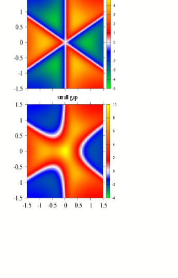
Figure 1: (Color online) Color plot of the orbital magnetic moment $m_{z}$ as a function of $k_{x}$ and $k_{y}$ in the surface state Brillouin zone with momentum in units of $nm^{-1}$. The top frame is for $\Delta=0$ and the bottom for $\Delta=0.1eV$. In both frames the hexagonal warping $\lambda=0.2$ in unit of $eV\cdot nm^{3}$.

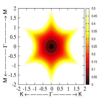
Figure 2: (Color online) Constant energy contours C for various values of the chemical potential $\mu$ as a function of momentum $k_{x}$, $k_{y}$ in the surface states Brillouin zone with momentum in units of $nm^{-1}$.

The Hamiltonian used by Fu Fu to describe the surface states band structure near the $\Gamma$ point in the surface Brillouin zone of a topological insulator is

$$H_{0}=\hbar v_{k}(k_{x}\sigma_{y}-k_{y}\sigma_{x})+\frac{\lambda}{2}(k_{+}^{3}+k_{-}^{3})\sigma_{z}+\Delta\sigma_{z}+E_{0}(\mathbf{k})$$ (1)

where $E_{0}(\mathbf{k})=\hbar^{2}k^{2}/(2m)$ is a quadratic term which gives the Dirac fermionic dispersion curves an hour glass shape and provides particle-hole asymmetry. The Dirac fermion velocity to second order is $v_{k}=v_{F}(1+\alpha k^{2})$ with $v_{F}$ the usual Fermi velocity measured to be $2.55eV\cdot\mathring{A}$ and $\alpha$ is a constant which is fit along with $m$ to the measured band structure in reference (Fu, ). The hexagonal warping parameter $\lambda=250eV\cdot\mathring{A}^{3}$. The $\sigma_{x}$, $\sigma_{y}$, $\sigma_{z}$ are the Pauli matrices here referring to spin, while in graphene these would relate instead to pseudospin. Finally $k_{\pm}=k_{x}\pm ik_{y}$ with $k_{x}$, $k_{y}$ momentum along $x$ and $y$ axis respectively. The energy spectrum associated with the Hamiltonian [Eq. (1)] is

$$\varepsilon_{\pm}(\mathbf{k})=E_{0}(\mathbf{k})\pm\sqrt{\hbar^{2}v_{k}^{2}k^{2}+(\lambda k^{3}\cos(3\theta)+\Delta)^{2}}$$ (2)

where $\theta$ is the polar angle defining the direction of $\mathbf{k}$ in the two dimensional surface state Brillouin zone. The wave function $u(\mathbf{k},s)$ defined by the equation $H_{0}u(\mathbf{k},\pm)=\varepsilon_{\pm}(\mathbf{k})u(\mathbf{k},\pm),$ is given by

$$u(\mathbf{k},s)=\frac{\hbar v_{k}k\left(1,\frac{\Delta(k,\theta)-s\sqrt{\hbar^{2}v_{k}^{2}k^{2}+(\Delta(k,\theta))^{2}}}{\hbar v_{k}}\frac{-ik_{x}+k_{y}}{k^{2}}\right)^{T}}{\sqrt{\hbar^{2}v_{k}^{2}k^{2}+(\Delta(k,\theta)-s\sqrt{\hbar^{2}v_{k}^{2}k^{2}+(\Delta(k,\theta))^{2}})^{2}}}$$ (3)

Here $s=+/-$ gives conduction and valence band respectively and $\Delta(k,\theta)=\Delta+\lambda k^{3}\cos(3\theta)\equiv\Delta+\lambda(k_{x}^{3}-3k_{x}k_{y}^{2})$. Note that the quadratic in momentum Schrödinger term $E_{0}(\mathbf{k})$ does not appear in the wave function. Introducing a unit vector $\hat{z}$ perpendicular to the surface plane, the Berry curvature associated with the wave function (for simplicity we set $v_{k}=v$) is given by

$$\Omega_{c}(\mathbf{k})=\hat{z}\cdot\nabla_{\mathbf{k}}\times\left\langle u(\mathbf{k},+)|i\nabla_{\mathbf{k}}|u(\mathbf{k},+)\right\rangle$$ (4)

$$= -\frac{\hbar^{2}v^{2}(\Delta-2\lambda k_{x}^{3}+6\lambda k_{x}k_{y}^{2})}{2[(\Delta+\lambda(k_{x}^{3}-3k_{x}k_{y}^{2}))^{2}+\hbar^{2}v^{2}k^{2}]^{3/2}}$$

for the conduction band and for the valence band $\Omega_{v}(\mathbf{k})=-\Omega_{c}(\mathbf{k})$.

Closely related to the Berry curvature is the orbital magnetic moment $m_{z}(\mathbf{k},s)$ which for the conduction band $s=+$ is given by Xiao1

$$m_{z}(\mathbf{k,+})$$ (5)

$$= -i(e/2\hbar)\{\hat{z}\cdot\left\langle\nabla_{\mathbf{k}}u(\mathbf{k},+)|\times[H_{0}-\varepsilon_{+}(k)]|\nabla_{\mathbf{k}}u(\mathbf{k},+)\right\rangle\}$$

$$= -(e/2\hbar)\frac{\hbar^{2}v^{2}(\Delta-2\lambda k_{x}^{3}+6\lambda k_{x}k_{y}^{2})}{[(\Delta+\lambda(k_{x}^{3}-3k_{x}k_{y}^{2}))^{2}+\hbar^{2}v^{2}k^{2}]}$$

and for the valence band $m_{z}(\mathbf{k},-)=m_{z}(\mathbf{k,+})$. Except for numerical factors this expression differs from the Eq. (4) for the Berry curvature only in its denominator which appears to power one rather than $3/2$. When we do not include a warping term in the Hamiltonian the Berry curvature as well as the orbital magnetic moment is proportional to the gap and would vanish for $\Delta=0$. This no longer is the case if warping is included. Even with $\Delta=0$ there is an orbital magnetic moment as we show in Fig. 1 which is a color plot of the magnitude of $m_{z}$ as a function of momentum ($k_{x}$, $k_{y}$) in the surface state Brillouin zone with momentum in units of $\pi$. We see that $m_{z}(k_{x},k_{y})$ is finite in most of the $k_{x}$-$k_{y}$ plane with zero along the lines of $\theta=\pm\pi/6$ and $\theta=\pi/2$. Thus $m_{z}(k_{x},k_{y})$ changes sign 6 times as $\theta$ ranges from $0$ to $2\pi$. This is in sharp contrast to the case when the hexagonal warping term is zero but the gap is finite. In this case $m_{z}(k,+)$ reduces to

$$-\frac{e}{2\hbar}\frac{\hbar^{2}v^{2}\Delta}{\Delta^{2}+\hbar^{2}v^{2}k^{2}}$$ (6)

which is isotropic in the $(k_{x},k_{y})$ plane and is peaked at $k=0$. In fact in the limit $\Delta\rightarrow 0$ we get $-\frac{e\pi}{2\hbar}\delta(k^{2})$. This maximum around the origin remains even when warping is included as we show in the color plot in the lower frame of Fig. 1 where a small gap $\Delta=0.1eV$ is included alongside a finite $\lambda$. The same value of $\lambda=0.2eV\cdot nm^{3}$ was used in both top and bottom frame. We note that now the contours of zero orbital magnetic moment are no longer straight lines and that we no longer have perfect symmetry between regions of positive and negative magnetic moments. The zero along $\theta=0,\pm 2\pi/3$ are at a finite value of the absolute momentum $k=(\Delta/(2\lambda))^{1/3}$ which represents the minimum value of momentum for which the magnetic moment can vanish whatever the direction of $\mathbf{k}$.

III Berry phase

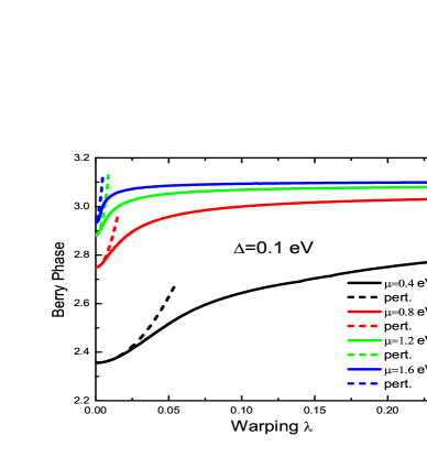
Figure 3: (Color online) Effect of warping on Berry phase. The Schrödinger term $E_{0}(k)=0$, the gap $\Delta=0.1eV$. Several values of chemical potential are considered and color coded. In all cases the dashed lines are our simplified results of Eq. (17) for the small $\lambda$ limit. The horizontal axis is $\lambda$ (warping) in unit of $eV\cdot nm^{3}$. The solid lines are from Eq. (12) evaluated numerically.

Based on the Berry curvature we can also calculate the Berry phase for a closed contour C, which is defined as

$$\Gamma_{s}(C)=\oint_{C}d\mathbf{k\cdot}\left\langle u(\mathbf{k},s)|i\nabla_{\mathbf{k}}|u(\mathbf{k},s)\right\rangle$$ (7)

By Stokes’ theorem we know that

$$\oint_{C}d\mathbf{k\cdot A=}\iint_{S}dk_{x}dk_{y}(\nabla\times\mathbf{A\cdot(-}\hat{z}))$$ (8)

We assume that the contour C is clockwise and the area enclosed by it is pointing in the negative $\hat{z}$ direction, and the chemical potential is positive for definiteness. Thus

$$\Gamma_{+}(C)=\iint_{S}dk_{x}dk_{y}\Theta(\mu-\varepsilon_{+}(\mathbf{k}))$$

$$\times\frac{\hbar^{2}v^{2}(\Delta-2\lambda k_{x}^{3}+6\lambda k_{x}k_{y}^{2})}{2[(\Delta+\lambda(k_{x}^{3}-3k_{x}k_{y}^{2}))^{2}+\hbar^{2}v^{2}k^{2}]^{3/2}}$$ (9)

where $\mu$ is the energy for the contour C. To see the effect of hexagonal warping on the Berry phase we start with no Schrödinger term $E_{0}(k)=0$ in Eq. (1). We get

$$\Gamma_{+}(C)=\int_{0}^{2\pi}d\theta\int_{0}^{k_{F}(\theta)}kdk$$

$$\times\frac{\hbar^{2}v^{2}(\Delta-2\lambda k^{3}\cos(3\theta))}{2[(\Delta+\lambda k^{3}\cos(3\theta))^{2}+\hbar^{2}v^{2}k^{2}]^{3/2}}$$ (10)

The integration over the magnitude of $k$ can be performed using the integral

$$\int\frac{(B-2Ak^{3})kdk}{[k^{2}+(B+Ak^{3})^{2}]^{3/2}}=\frac{-(B+Ak^{3})}{\sqrt{k^{2}+(B+Ak^{3})^{2}}}$$ (11)

and we get

$$\Gamma_{+}(C)$$ (12)

$$= \int_{0}^{2\pi}d\theta\frac{-(\Delta+\lambda k^{3}\cos(3\theta))}{2[(\Delta+\lambda k^{3}\cos(3\theta))^{2}+\hbar^{2}v^{2}k^{2}]^{1/2}}|_{0}^{k_{F}(\theta)}$$

$$= \frac{1}{2}\int_{0}^{2\pi}d\theta\{sign(\Delta)-\frac{(\Delta+\lambda k_{F}^{3}(\theta)\cos(3\theta))}{\mu}\}$$

where $k_{F}(\theta)$ is determined by

$$\sqrt{(\Delta+\lambda k_{F}^{3}(\theta)\cos(3\theta))^{2}+\hbar^{2}v^{2}k_{F}^{2}(\theta)}=\mu.$$

Several limits of this expression should be emphasized. First in the limit of $\mu\rightarrow\infty$ we get a Berry phase of $\pi sign(\Delta)$ and this is the same value as when $\lambda=0$ i.e. no warping is included. While warping does not change the Berry phase when the contour has $\mu\rightarrow\infty$ it does change it for any finite $\mu$. We can get an analytic expression for this change in the limit of $\lambda\rightarrow 0$ retaining lowest order.

To evaluate the Berry phase Eq. (12) we need to know the fermi momentum $k_{F}$ as a function of angle $\theta$. We show such contours in Fig. 2 for various values of $\mu$. At small $\mu$ the contour is nearly circular and distorts into a snowflake shape as $\mu$ increases. We can solve for $k_{F}(\theta)$ v.s. angle $\theta$. Keeping only lowest significant order in $\lambda$ for small $\lambda$, the equation to be solved is

$$(\Delta+\lambda k_{F}^{3}(\theta)\cos(3\theta))^{2}+\hbar^{2}v^{2}k_{F}^{2}(\theta)=\mu^{2}$$ (13)

which is a cubic equation for $k_{F}(\theta)$. For $\lambda=0$ (no warping) $k_{F}$ is isotropic and equals $\sqrt{\mu^{2}-\Delta^{2}}/(\hbar v)$. We can use this in Eq. (13) to get a first order correction to $k_{F}(\theta)$

$$\hbar^{2}v^{2}\frac{k_{F}^{2}(\theta)}{\mu^{2}}\cong 1-\frac{\Delta^{2}}{\mu^{2}}-2\frac{\Delta}{\mu}\frac{\lambda}{\mu}(\frac{\mu^{2}-\Delta^{2}}{\hbar^{2}v^{2}})^{3/2}\cos(3\theta)$$ (14)

from which we obtain

$$k_{F}^{3}(\theta)\cong(\frac{\mu}{\hbar v})^{3}(\frac{\mu^{2}-\Delta^{2}}{\mu^{2}})^{3/2}$$

$$\times[1-3\frac{\lambda\mu\Delta}{(\hbar v)^{3}}\sqrt{\frac{\mu^{2}-\Delta^{2}}{\mu^{2}}}\cos(3\theta)]$$ (15)

This gives a Berry phase

$$\Gamma_{+}(C)=\frac{1}{2}\int_{0}^{2\pi}d\theta\{sign(\Delta)-\frac{\Delta}{\mu}-\frac{\lambda}{\mu}\cos(3\theta)(\frac{\mu}{\hbar v})^{3}$$

$$\times(\frac{\mu^{2}-\Delta^{2}}{\mu^{2}})^{3/2}[1-3\frac{\lambda\mu\Delta}{(\hbar v)^{3}}\sqrt{\frac{\mu^{2}-\Delta^{2}}{\mu^{2}}}\cos(3\theta)]\}$$ (16)

The one in the last bracket will give zero after integration over angle $\theta$ because this term is linear in $\cos(3\theta)$ which averages to zero. The second term however involves $\int_{0}^{2\pi}d\theta\cos^{2}(3\theta)$ which is non-zero and equal to $\pi$. Therefore

$$\Gamma_{+}(C)=\pi[sign(\Delta)-\frac{\Delta}{\mu}(1-\frac{3}{2}\frac{\lambda^{2}(\mu^{2}-\Delta^{2})^{2}}{(\hbar v)^{6}})]$$ (17)

In Fig. 3 we show numerical results for $\Gamma_{+}(C)$ as a function of warping $\lambda$ for various values of chemical potential $\mu$ namely $\mu=0.4eV$ (black), $\mu=0.8eV$ (red), $\mu=1.2eV$ (green), $\mu=1.6eV$ (blue). In all cases $\Delta=0.1eV$. The solid curve are exact numerical results based on Eq. (12) while the dashed curves are the approximate result of Eq. (17). We see that both sets agree perfectly at small $\lambda$ but begin to deviate significantly as $\lambda$ increases. In the limit of large $\lambda$ the Berry phase goes towards its $\Delta=0$ value of $\pi$.

When $\lambda=0$

$$\Gamma_{+}(C)=\pi(sign(\Delta)-\frac{\Delta}{\mu})$$ (18)

which is a known result. Another known result can also be verified. If we set $\hbar=1$ for simplicity and retain the Schrödinger term $E_{0}(\mathbf{k})$ of Eq. (1) we can solve for $k_{F}$

$$k_{F}^{2}=2\mu m+2m^{2}v^{2}-2m^{2}\sqrt{2\frac{\mu}{m}v^{2}+v^{4}+\frac{\Delta^{2}}{m^{2}}}$$ (19)

and so

$$\sqrt{v^{2}k_{F}^{2}+\Delta^{2}}=\mu-k_{F}^{2}/2m$$ (20)

$$= -mv^{2}+mv^{2}\sqrt{1+\frac{2\mu}{mv^{2}}+\frac{\Delta^{2}}{(mv^{2})^{2}}}$$

which gives the Berry phase

$$\Gamma_{+}(C)=\pi[1-\frac{\Delta}{\sqrt{v^{2}k_{F}^{2}+\Delta^{2}}}]$$ (21)

$$= \pi[1+\frac{\Delta}{mv^{2}[1-\sqrt{1+\frac{2\mu}{mv^{2}}+\frac{\Delta^{2}}{(mv^{2})^{2}}}]}]$$

This result was obtained by Wright and Mckenzie.Wright1 ; Fuchs ; Wright2

IV Spin texture

Figure 4: Spin texture ($S_{x}$,$S_{y}$) in the $k_{x}$-$k_{y}$ plane of the surface state Brillouin zone. The units of momentum are $nm^{-1}$. The gap $\Delta=0.1eV$ and the warping $\lambda=0.2eV\cdot nm^{3}$.

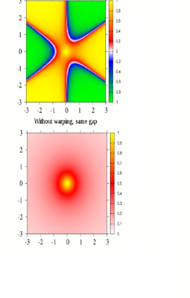
Figure 5: (Color online) The z component of spin ($S_{z}$, in units of $\hbar/2$) perpendicular to surface as a function of $k_{x}$, $k_{y}$ in units of $nm^{-1}$ in the 2-D surface state Brillouin zone, with (top frame) and without (bottom frame) warping. The gap $\Delta=0.1eV$ and in the top frame the warping $\lambda=0.2eV\cdot nm^{3}$.

The Pauli matrix in Eq. (1) refer to spin. From a knowledge of the wave function given in Eq. (3), we can compute the average value of the electron spin components $S_{x}$, $S_{y}$ (in plane) and $S_{z}$ (out of plane). The results are

$$S_{x} = \frac{\hbar}{2}\langle u(\mathbf{k},\pm)|\sigma_{x}|u(\mathbf{k},\pm)\rangle$$ (22)

$$= \pm\frac{\hbar}{2}\frac{-\hbar vk_{y}}{\sqrt{(\Delta+\lambda(k_{x}^{3}-3k_{x}k_{y}^{2}))^{2}+\hbar^{2}v^{2}k^{2}}}$$

$$S_{y} = \frac{\hbar}{2}\langle u(\mathbf{k},\pm)|\sigma_{y}|u(\mathbf{k},\pm)\rangle$$ (23)

$$= \pm\frac{\hbar}{2}\frac{\hbar vk_{x}}{\sqrt{(\Delta+\lambda(k_{x}^{3}-3k_{x}k_{y}^{2}))^{2}+\hbar^{2}v^{2}k^{2}}}$$

$$S_{z} = \frac{\hbar}{2}\langle u(\mathbf{k},\pm)|\sigma_{z}|u(\mathbf{k},\pm)\rangle$$ (24)

$$= \pm\frac{\hbar}{2}\frac{\Delta+\lambda(k_{x}^{3}-3k_{x}k_{y}^{2})}{\sqrt{(\Delta+\lambda(k_{x}^{3}-3k_{x}k_{y}^{2}))^{2}+\hbar^{2}v^{2}k^{2}}}.$$

We show our results in Fig. 4 for the $S_{x}$, $S_{y}$ component in the $k_{x}$, $k_{y}$ plane with momentum measured in units of $nm^{-1}$. We see that the in-plane component of spin remains locked perpendicular to its momentum Hsieh1 ; Hsieh2 ; Xu1 ; Xu2 but its magnitude is no longer independent of angle $\theta$. Basak et.al Basak have gone beyond the Hamiltonian (1) to include a fifth order spin-orbit coupling which could exist at the surface of a rhombohedral crystal. This lifts the momentum spin locking found here but goes beyond the present discussion. For $\lambda=0$ we have

$$S_{x} = \pm\frac{\hbar}{2}\frac{-\hbar vk_{y}}{\sqrt{\Delta^{2}+\hbar^{2}v^{2}k^{2}}}$$

$$S_{y} = \pm\frac{\hbar}{2}\frac{\hbar vk_{x}}{\sqrt{\Delta^{2}+\hbar^{2}v^{2}k^{2}}}.$$ (25)

and hence

$$\sqrt{S_{x}^{2}+S_{y}^{2}}=\frac{\hbar}{2}\frac{\hbar vk}{\sqrt{\Delta^{2}+\hbar^{2}v^{2}k^{2}}}$$ (26)

which reduces to $\frac{\hbar}{2}$ independent of $k$ when there is no gap. With a gap $\sqrt{S_{x}^{2}+S_{y}^{2}}=0$ at $k=0$ and saturates to value $\frac{\hbar}{2}$ at $k\rightarrow\infty$. These results imply that the z component of spin is also modified by the presence of the gap and that there are further modifications when $\lambda\neq 0$. Returning to the results of Fig. 4 and Eq. (22) and (23), we get for the magnitude of the in plane component of spin with warping

$$\sqrt{S_{x}^{2}+S_{y}^{2}}=\frac{\hbar}{2}\frac{\hbar vk}{\sqrt{(\Delta+\lambda(k_{x}^{3}-3k_{x}k_{y}^{2}))^{2}+\hbar^{2}v^{2}k^{2}}}$$ (27)

For $k$ very large this no longer saturates to a value of $\frac{\hbar}{2}$ but tends to zero because of the $k^{3}$ dependence in the denominator. For $k\rightarrow 0$ however the in plane component of spin remains zero as we found for the $\lambda=0$ case. Both these limiting behavior are clearly seen in Fig. 4. For a general value of $\mathbf{k}$ there is a great deal of anisotropy in the magnitude of the in plane spin component. It is maximum for $\theta=\pi/3$ or $\pi$ and minimum for $\theta=\pm 2\pi/3$ and $0$. Turning next to the z-component of spin, note from Eq. (24) that with $\Delta=0$ and $\lambda=0$, the z-component of spin $S_{z}=0$. But $S_{z}$ is no longer zero when hexagonal warping is non-zero even for $\Delta=0$. The numerator in Eq. (24) is proportional to $\lambda k^{3}cos(3\theta)$ and, as for the orbital magnetic moment we get zero only along $\theta=\pm\pi/6$ and $\pi/2$. The z-component of spin is otherwise finite and has regions where it is positive and other regions where it is negative. There is no need to introduce magnetic dopants in the system to see these effects. When a finite gap is opened the spin texture for $S_{z}$ becomes even more complicated. In this case a color plot of the value of the z-component of spin given in Eq. (24) is presented in the top frame of Fig. 5. It has a maximum of $\frac{\hbar}{2}$ at $k=0$ where the in plane spin is zero and at larger $k$ values has three contours of zeros, different from the contours of zero found in Fig. 1 for the orbital magnetic moment. In the first case the zeros correspond to the zeros of the equation $\Delta+\lambda k^{3}\cos(3\theta)=0$ and in the second it is $\Delta-2\lambda k^{3}\cos(3\theta)=0$. In contrast for $\lambda=0$ the spin structure for the $S_{z}$ component of spin is isotropic and given by

$$S_{z}=\pm\frac{\hbar}{2}\frac{\Delta}{\sqrt{\Delta^{2}+\hbar^{2}v^{2}k^{2}}}$$ (28)

a color plot of the magnitude of $S_{z}$ as a function of $k_{x}$ and $k_{y}$ is found in the lower frame of Fig. 5 and is for comparison with the top frame. Only the region near $k=0$ is unaffected by the hexagonal warping. For the isotropic case ($\lambda=0$, no hexagonal warping) we can easily see that the Berry phase $\Gamma_{+}(C)$ defined in Eq. (18) for pure Dirac and in Eq. (21) when there is a mass term, are reproduced when the z-component of spin given by (28) is averaged over the Fermi surface i.e.

$$1-\Gamma_{+}(C)/\pi=\left\langle S_{z}\right\rangle_{\mu}\equiv\frac{\int d^{2}kS_{z}\delta(\mu-\varepsilon_{+}(\mathbf{k}))}{\int d^{2}k\delta(\mu-\varepsilon_{+}(\mathbf{k}))}$$ (29)

Even when warping is included we find numerically that this relationship remains very nearly true as can be seen in Fig. 6 where we compare $1-\left\langle S_{z}\right\rangle_{\mu}$ (solid curve) with $\Gamma_{+}(C)/\pi$ (dashed curve) as a function of chemical potential $\mu$ for four cases. The blue curves are for reference only and have no warping and no Schrödinger. The red are for m=infinity and $\lambda=0.2$. Dashed and solid curve deviate slightly from each other but the correlation remains excellent. The green and black curves have a mass $m=m_{e}$ (electron mass) and $m=0.1m_{e}$ respectively. The deviation between Berry phase and $\left\langle S_{z}\right\rangle_{\mu}$ decreases with increasing $m$. A measurement of $\Gamma_{+}(C)/\pi$ is equivalent to a measurement of $\left\langle S_{z}\right\rangle_{\mu}$ and vice versa.

V Circular polarization and dichroism

To calculate the interband optical matrix element we need the velocity components related to

$$\frac{\partial H}{\partial k_{x}}=\left(\begin{array}[]{cc}\lambda(3k_{x}^{2}-3k_{y}^{2})&-i\hbar v_{k}\\ i\hbar v_{k}&-\lambda(3k_{x}^{2}-3k_{y}^{2})\end{array}\right)$$ (30a)

and

$$\frac{\partial H}{\partial k_{y}}=\left(\begin{array}[]{cc}-6\lambda k_{x}k_{y}&-\hbar v_{k}\\ -\hbar v_{k}&6\lambda k_{x}k_{y}\end{array}\right).$$ (30b)

From this information we can work out the optical matrix element for valence (v) to conduction band (c). By definition Xiao2 ; Yao

$$\mathbf{P}^{cv}(\mathbf{k})=\left\langle u(\mathbf{k},+)|\nabla_{\mathbf{k}}H|u(\mathbf{k},-)\right\rangle.$$ (31)

After considerable but straightforward algebra we find that the square of the right and left polarization optical matrix elements are

$$|P_{+}^{cv}(\mathbf{k})|^{2} = \hbar^{2}v^{2}\{[\frac{\Delta-2\lambda(k_{x}^{3}-3k_{x}k_{y}^{2})}{\sqrt{\hbar^{2}v^{2}k^{2}+(\Delta+\lambda k_{x}^{3}-3\lambda k_{x}k_{y}^{2})^{2}}}+1]^{2}$$ (32)

$$+\frac{9\lambda^{2}(k_{y}^{3}-3k_{x}^{2}k_{y})^{2}}{\hbar^{2}v^{2}k^{2}+(\Delta+\lambda k_{x}^{3}-3\lambda k_{x}k_{y}^{2})^{2}}\}$$

$$|P_{-}^{cv}(\mathbf{k})|^{2} = \hbar^{2}v^{2}\{[\frac{-\Delta+2\lambda(k_{x}^{3}-3k_{x}k_{y}^{2})}{\sqrt{\hbar^{2}v^{2}k^{2}+(\Delta+\lambda k_{x}^{3}-3\lambda k_{x}k_{y}^{2})^{2}}}+1]^{2}$$ (33)

$$+\frac{9\lambda^{2}(k_{y}^{3}-3k_{x}^{2}k_{y})^{2}}{\hbar^{2}v^{2}k^{2}+(\Delta+\lambda k_{x}^{3}-3\lambda k_{x}k_{y}^{2})^{2}}\}$$

The difference between $|P_{+}^{cv}(\mathbf{k})|^{2}$ and $|P_{-}^{cv}(\mathbf{k})|^{2}$ works out to be

$$|P_{+}^{cv}(\mathbf{k})|^{2}-|P_{-}^{cv}(\mathbf{k})|^{2}$$ (34)

$$= 4\hbar^{2}v^{2}\frac{\Delta-2\lambda(k_{x}^{3}-3k_{x}k_{y}^{2})}{\sqrt{\hbar^{2}v^{2}k^{2}+(\Delta+\lambda k_{x}^{3}-3\lambda k_{x}k_{y}^{2})^{2}}}$$

which can be written in terms of the orbital magnetic moment Eq. (5) as

$$|P_{+}^{cv}(\mathbf{k})|^{2}-|P_{-}^{cv}(\mathbf{k})|^{2}=-4\frac{\hbar}{e}m_{z}(\mathbf{k})[\varepsilon_{+}(\mathbf{k)-}\varepsilon_{-}(\mathbf{k)}]$$ (35)

We can also work out the sum of $|P_{+}^{cv}(\mathbf{k})|^{2}+|P_{-}^{cv}(\mathbf{k})|^{2}$, to get

$$|P_{+}^{cv}(\mathbf{k})|^{2}+|P_{-}^{cv}(\mathbf{k})|^{2}$$ (36)

$$= 2v^{2}\hbar^{2}/[\hbar^{2}v^{2}k^{2}+(\Delta+\lambda k_{x}^{3}-3\lambda k_{x}k_{y}^{2})^{2}]\times$$

$$[\lambda^{2}(5k_{x}^{6}+51k_{x}^{4}k_{y}^{2}-9k_{x}^{2}k_{y}^{4}+9k_{y}^{6})$$

$$-2\Delta\lambda(k_{x}^{3}-3k_{x}k_{y}^{2})+2\Delta^{2}+\hbar^{2}v^{2}k^{2}]$$

which can be rewritten as

$$| P_{+}^{cv}(\mathbf{k})|^{2}+|P_{-}^{cv}(\mathbf{k})|^{2}=[\varepsilon_{+}(\mathbf{k)-}\varepsilon_{-}(\mathbf{k)]\times}$$ (37)

$$[\frac{\partial^{2}[\varepsilon_{+}(\mathbf{k})-E_{0}(\mathbf{k})]}{\partial k_{x}^{2}}+\frac{\partial^{2}[\varepsilon_{+}(\mathbf{k})-E_{0}(\mathbf{k})]}{\partial k_{y}^{2}}]$$

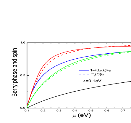
Figure 6: (Color online) The Berry phase $\Gamma_{+}(C)$ of Eq. (7) normalized by $\pi$ (dashed lines) compared with one minus the Fermi surface average z-component of spin $\left\langle S_{z}\right\rangle_{\mu}$ defined in Eq. (29) (solid lines) as a function of chemical potential $\mu$. The blue curves are for comparison and give results for the isotropic case $\lambda=0$ (no warping). The Berry phase and spin agree perfectly in this case. The gap is set at 0.1eV in all cases. The other curves are for a warping of $\lambda=0.2eV(nm)^{3}$. The red curves have no Schrödinger quadratic piece ($E_{0}(k)=0$ in Eq. (1)), while the green are for $m=m_{e}$ (bare electron mass) and the black for $m=0.1m_{e}$. The derivations between dash and solid curves are always small and are reduced as $m$ is decreased.

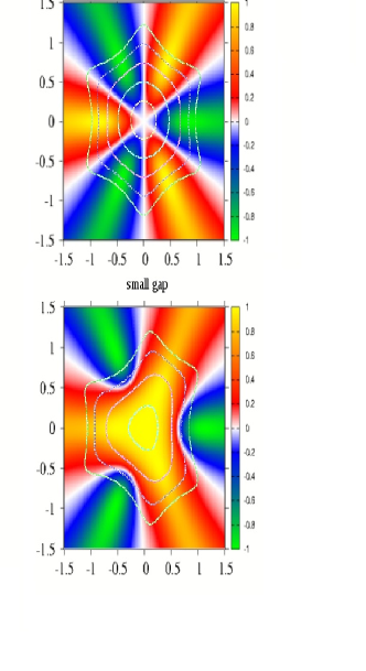
Figure 7: (Color online) Color plots for the degree of circular polarization $\eta(\mathbf{k})$ defined in Eq. (38) as a function of $k_{x}$, $k_{y}$ in units of $nm^{-1}$ in the 2-D surface state Brillouin zone. The contours (white lines) are added for several values of the chemical potential (fermi surface). In the top frame $\Delta=0$ and fermi contours go from circle to snowflakes. In the lower frame the opening of a gap $\Delta=0.1eV$ distorts the fermi contours.

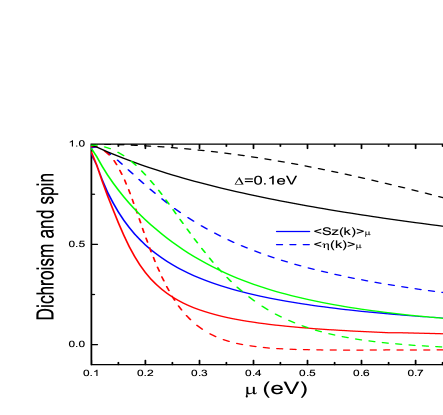
Figure 8: (Color online) Comparison of dichroism $\left\langle\eta(\mathbf{k})\right\rangle_{\mu}$ defined in Eq. (39) (dashed curves) and the Fermi surface averaged z-component of spin $\left\langle S_{z}(\mathbf{k})\right\rangle_{\mu}$ (solid curves) defined in Eq. (29) as a function of chemical potential $\mu$. The blue curves are for no Schrödinger piece included in the Hamiltonian (1) i.e. $E_{0}(k)=0$, and no hexagonal warping ($\lambda=0$) and are for comparison. There is some correlation between spin-z and dichroism, both decrease monotonically with increasing $\mu$ and at $\mu=0.8eV$ differ by a factor of 2. The red curves have $\lambda=0.2eV(nm)^{3}$ as have all others and also have $E_{0}(k)=0$. The green curves include a Schrödinger piece with $m=m_{e}$ and the black are for $m=0.1m_{e}$. In no case is the correlation between spin and dichroism as good as that found in Fig. 6 for spin and Berry phase.

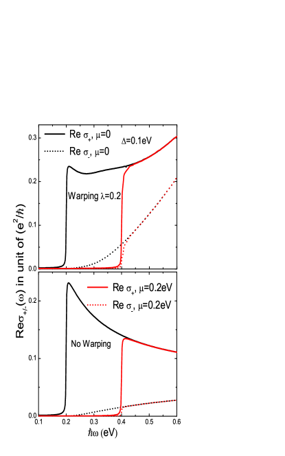
Figure 9: (Color online) AC optical conductivity (in units of $e^{2}/\hbar$) for circular polarized light as a function of photon energy $\omega$ in eV. A gap of 0.1eV is included. The top frame includes a warping term of $0.2eV\cdot nm^{3}$ and the bottom frame has no warping and is for comparison. Two value of chemical potential are shown as well as right $\sigma_{+}$ (solid) and left hand $\sigma_{-}$ (dotted) polarization.

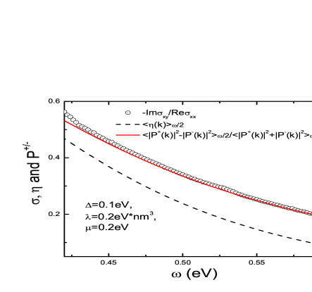
Figure 10: (Color online) The ratio $-Im\sigma_{xy}/Re\sigma_{xx}$ of Hall to longitudinal AC optical conductivity (open circles) as a function of photon energy $\omega$ above the interband absorption edge seen in Fig. 9. The parameters are gap $\Delta=0.1eV$, hexagonal warping $\lambda=0.2eV(nm)^{3}$ and chemical potential 0.2eV as in Fig. 9. Also shown as the dashed black curve is the average of the dichroism factor $\eta(\mathbf{k})$ over a surface of energy $\omega/2$. This quantity differs substantially from the open circles. On the other hand, the red line agrees very well with the open circles and is defined as the ratio of the average over a surface of energy $\omega/2$ of $|P_{+}^{cv}(\mathbf{k})|^{2}-|P_{-}^{cv}(\mathbf{k})|^{2}$ and $|P_{+}^{cv}(\mathbf{k})|^{2}+|P_{-}^{cv}(\mathbf{k})|^{2}$ separately as defined in Eq. (40).

The degree of circular polarization is therefore given by Xiao2 ; Yao ; Ezawa

$$\eta(\mathbf{k}) = \frac{|P_{+}^{cv}(\mathbf{k})|^{2}-|P_{-}^{cv}(\mathbf{k})|^{2}}{|P_{+}^{cv}(\mathbf{k})|^{2}+|P_{-}^{cv}(\mathbf{k})|^{2}}$$ (38)

$$= -\frac{-4\frac{\hbar}{e}m_{z}(\mathbf{k})}{[\frac{\partial^{2}[\varepsilon_{+}(\mathbf{k})-E_{0}(\mathbf{k})]}{\partial k_{x}^{2}}+\frac{\partial^{2}[\varepsilon_{+}(\mathbf{k})-E_{0}(\mathbf{k})]}{\partial k_{y}^{2}}]}$$

We note first that $\eta(\mathbf{k})$ is proportional to the orbital magnetic moment and is further divided by the appropriate sum of the second derivative of the energy $\varepsilon_{+}(\mathbf{k})-E_{0}(\mathbf{k})$ with respect to $k_{x}$ and $k_{y}$ respectively. While the energy $\varepsilon_{+}(\mathbf{k})$ depends on $E_{0}(\mathbf{k})$ the quadratic Schrödinger contribution to the Hamiltonian, the difference $\varepsilon_{+}(\mathbf{k})-E_{0}(\mathbf{k})$ does not and so the entire expression Eq. (38) for $\eta(\mathbf{k})$ is completely independent of this term. We show a color plot for the magnitude of $\eta(\mathbf{k})$ as a function of $k_{x}$, $k_{y}$ in the 2-D surface state Brillouin zone in Fig.  7. For a fix value of the absolute value of the momentum the zeros in $\eta(\mathbf{k})$ (top frame) are at the same angles as for the orbital magnetic moment of Fig. 1. The top frame of Fig. 7 is for a case where $\Delta=0$ (no gap) while the bottom frame has a finite gap $\Delta=0.1eV$. In the case $\Delta=0$ averaging over angles at fixed $k$ will give zero by symmetry because the numerator of Eq. (5) have the form $2\lambda k^{3}\cos(3\theta)$. Similar results appear in Fig. 5 of a paper by Liu et.al. Liu Here we are mainly interested in the case when the gap $\Delta$ is non zero which is very different. When a gap is included the numerator is instead $\Delta-2\lambda k^{3}\cos(3\theta)$, so that now we get a non zero result proportional to the gap $\Delta$. Effectively the hexagonal warping term has averaged to zero in the numerator leaving a single term. This term however retains some knowledge of the warping as its contribution remains in the denominator of Eq. (38) and of Eq. (5).

Interband optical absorption from a state $\mathbf{k}$ in the valence band to a state $\mathbf{k}$ in the conduction band will involve $|P_{+}^{cv}(\mathbf{k})|^{2}$ and $|P_{-}^{cv}(\mathbf{k})|^{2}$ for right and left circular polarized light respectively and $\eta(\mathbf{k})$ then measures the difference in absorption between these two cases. For a given value of chemical potential $\mu>0$ there is an absorption edge at $2\mu$ and the momentum involved is $k_{F}(\theta)$ which we show in Fig. 7 as white contours which start as circles for $\mu\rightarrow 0$ and distort to a more and more cusped snowflake as $\mu$ is increased (top frame). When a gap is included the Fermi surface distorts further as is shown in the lower frame (white contours) and has reduced symmetry. At the same time the color plot for $\eta(\mathbf{k})$ also shows reduced symmetry as compared with the top frame. These anisotropies have consequences for interband optical absorption.

It is useful to introduce an average over a constant energy surface of the circular polarization $\eta(\mathbf{k})$ defined in Eq. (38) as this quantity is more closely connected with the circular dichroism of the AC conductivity. We define

$$\langle\eta(\mathbf{k})\rangle_{\omega/2}\equiv\frac{\int d^{2}k\eta(\mathbf{k})\delta(\omega-2\varepsilon(\mathbf{k}))}{\int d^{2}k\delta(\omega-2\varepsilon(\mathbf{k}))}$$ (39)

where $\varepsilon(\mathbf{k})=\sqrt{\hbar^{2}v_{k}^{2}k^{2}+(\lambda k^{3}\cos(3\theta)+\Delta)^{2}}$ which describes the energy involved in interband transitions from valence to conduction band namely $2\varepsilon(\mathbf{k})\equiv\varepsilon_{+}(\mathbf{k})-\varepsilon_{-}(\mathbf{k})$ where $\varepsilon_{\pm}(\mathbf{k})$ is defined in Eq. (2). Related quantities are the separate averages of sum and difference $|P^{+}(\mathbf{k})|^{2}$ and $|P^{-}(\mathbf{k})|^{2}$ defined in Eq. (34) and (36) respectively. These are

$$\langle|P^{+}(\mathbf{k})|^{2}\pm|P^{-}(\mathbf{k})|^{2}\rangle_{\omega/2}$$ (40)

$$\equiv \frac{\int d^{2}k[|P^{+}(\mathbf{k})|^{2}\pm|P^{-}(\mathbf{k})|^{2}]\delta(\omega-2\varepsilon(\mathbf{k}))}{\int d^{2}k\delta(\omega-2\varepsilon(\mathbf{k}))}$$

Numerical results for the averaged circular dichroism $\langle\eta(\mathbf{k})\rangle_{\omega/2\equiv\mu}$ defined in (39) are presented in Fig. 8 as dashed lines as a function of energy $\mu$. In all cases the gap $\Delta=0.1eV$. For the blue curve no Schrödinger term is included i.e. $E_{0}(k)=0$ in the Hamiltonian (1), and there is no hexagonal warping ($\lambda=0$) and provides the isotropic limit as a reference for the rest of the curves. It shows a monotonic decrease of $\langle\eta(\mathbf{k})\rangle_{\omega/2}$ as a function of $\mu$. When a hexagonal warping term of $\lambda=0.2eV\cdot nm^{2}$ is included we obtain the red curve which shows that the dichroism is greatly reduced over its isotropic value and is very small for values of $\mu$ greater than about $0.3eV$. If however, in addition to the warping we include a Schrödinger term with $m=m_{e}$ (with $m_{e}$ the bare electron mass) we obtain the green dashed curve which has moved closer to the isotropic results than is the case for the red curve. If we make the Schrödinger piece $E_{0}(k)$ in (1) even larger by taking $m=0.1m_{e}$ we get the black dashed curve which shows that now $\langle\eta(\mathbf{k})\rangle_{\omega/2\equiv\mu}$ remains much closer to one and is still of order $0.8$ at $\mu=0.8eV$.

It is of interest to compare these results for $\langle\eta(\mathbf{k})\rangle_{\omega/2}$ with our previous results for the Fermi surface average of the z-component of spin $\left\langle S_{z}\right\rangle_{\mu}$ defined in Eq. (29). These are shown as the solid curves in Fig. 8 which are color coded to match the dashed curves. In all cases we note some correlation between dichroism defined by Eq. (39) and the average of the z-component of spin. Both decrease monotonically with increasing $\mu$ but in all cases there are significant quantitative differences and contrary to what was found before when spin and Berry phase were compared the dichroism does not translate directly into a quantitative measure of $\left\langle S_{z}\right\rangle_{\mu}$. Here we are describing the dichroism associated with the absorption of light. Similar issues arise and have been studied extensively when spin polarized angular resolved photoemission is considered. Henk In that case a photon enters the sample and a photo electron is detected. Usually one concentrates on the electron spectral density as the outcome of such experiments. But the optical matrix element between incident light and electron also enters and can have an effect on the ejected electron. Herdt ; Nomura ; Yang

To calculate in AC optical absorption we need to consider the Kubo formula for longitudinal $\sigma_{xx}(\omega)$ and transverse $\sigma_{xy}(\omega)$ conductivity. In terms of the matrix Green’s function $\widehat{G}(\mathbf{k,}\omega_{l})$ in Matsubara notation with $\omega_{n}=(2n+1)\pi T$ and $\omega_{l}=2l\pi T$ the Fermion and Boson Matsubara frequencies, $n$ and $l$ are integers, $T$ is the temperature and $Tr$ is a trace, the longitudinal conductivity for gapped Dirac fermion with warping is given by

$$\sigma_{xx}(\omega)=\frac{e^{2}}{i\omega}\frac{1}{4\pi^{2}}\int_{0}^{k_{cut}}kdkd\theta\times$$

$$T\sum_{l}Tr\langle v_{x}\widehat{G}(\mathbf{k,}\omega_{l})v_{x}\widehat{G}(\mathbf{k,}\omega_{n}+\omega_{l})\rangle_{\omega_{n}\rightarrow\omega+i\delta}$$ (41)

which works out to be

$$\sigma_{xx}(\omega)=-\frac{e^{2}}{i\omega}\frac{1}{4\pi^{2}}\int_{0}^{k_{cut}}\frac{kdkd\theta H(\theta)}{v_{k}^{2}k^{2}+(\Delta+\lambda k^{3}\cos(3\theta))^{2}}$$

$$[\frac{f(\varepsilon_{-})-f(\varepsilon_{+})}{\omega-2\sqrt{v_{k}^{2}k^{2}+(\Delta+\lambda k^{3}\cos(3\theta))^{2}}+i\delta}$$

$$-\frac{f(\varepsilon_{-})-f(\varepsilon_{+})}{\omega+2\sqrt{v_{k}^{2}k^{2}+(\Delta+\lambda k^{3}\cos(3\theta))^{2}}+i\delta}]$$ (42)

where

$$H(\theta)=9\lambda^{2}v_{k}^{2}k^{6}\cos^{2}(2\theta)+v_{k}^{4}k^{2}\sin^{2}\theta$$

$$+v_{k}^{2}(\Delta+\lambda k^{3}\cos(3\theta))^{2}$$

$$-2\times 3v_{k}^{2}\lambda k^{3}\cos(2\theta)\cos\theta[\Delta+\lambda k^{3}\cos(3\theta)]$$ (43)

From the matrix elements we have

$$\sigma_{xx}(\omega)=-\frac{e^{2}}{i\omega}\frac{1}{4\pi^{2}}\int_{0}^{k_{cut}}kdkd\theta|P_{x}^{cv}(\mathbf{k})|^{2}$$

$$[\frac{f(\varepsilon_{-})-f(\varepsilon_{+})}{\omega-2\sqrt{v_{k}^{2}k^{2}+(\Delta+\lambda k^{3}\cos(3\theta))^{2}}+i\delta}$$

$$-\frac{f(\varepsilon_{-})-f(\varepsilon_{+})}{\omega+2\sqrt{v_{k}^{2}k^{2}+(\Delta+\lambda k^{3}\cos(3\theta))^{2}}+i\delta}]$$ (44)

The transverse Hall conductivity is given by

$$\sigma_{xy}(\omega)=\frac{e^{2}}{i\omega}\frac{1}{4\pi^{2}}\int_{0}^{k_{cut}}kdkd\theta\times$$

$$T\sum_{l}Tr\langle v_{x}\widehat{G}(\mathbf{k,}\omega_{l})v_{y}\widehat{G}(\mathbf{k,}\omega_{n}+\omega_{l})\rangle_{\omega_{n}\rightarrow\omega+i\delta}$$ (45)

which can be reduced to Xiao3

$$\sigma_{xy}(\omega)=\frac{e^{2}}{\omega}\frac{1}{4\pi^{2}}\int_{0}^{k_{cut}}\frac{kdkd\theta v_{k}^{2}[\Delta-2\lambda k^{3}\cos(3\theta)]}{\sqrt{v_{k}^{2}k^{2}+(\Delta+\lambda k^{3}\cos(3\theta))^{2}}}$$

$$[\frac{f(\varepsilon_{-})-f(\varepsilon_{+})}{\omega-\varepsilon_{+}+\varepsilon_{-}+i\delta}+\frac{f(\varepsilon_{-})-f(\varepsilon_{+})}{\omega-\varepsilon_{-}+\varepsilon_{+}+i\delta}]\}$$ (46)

Results for the real part (absorptive part) of the circular polarized conductivity [$\sigma_{\pm}(\omega)\equiv\sigma_{xx}(\omega)\pm i\sigma_{xy}(\omega)$] $Re\sigma_{\pm}(\omega)$ are shown in Fig. 9. Both frames include a gap $\Delta=0.1eV$ and the warping parameter $\lambda$ was set at $0.2eV\cdot nm^{3}$. The vertical axis is for $Re\sigma_{\pm}(\omega)$ in units of $\frac{e^{2}}{\hbar}$ and the horizontal axis is photon energy in units of ($eV$). The solid lines are for $Re\sigma_{+}(\omega)$ while the dotted lines are for $Re\sigma_{-}(\omega)$, black is for a chemical potential $\mu=0$ and red for $\mu=0.2eV$. Comparing top and bottom frame we wish to emphasize two features. First, hexagonal warping leads to an increasing absorption for $\omega$ greater than its threshold value in the solid curves for right circular polarized light $Re\sigma_{+}(\omega)$ (top frame) in contrast to the case without warping (bottom frame) where a decreasing absorption is seen. Note that for $\mu=0$ the absorption edge is determined by the gap and falls at $2\Delta=0.2eV$. For $\mu=0.2eV$ it is at $2\mu=0.4eV$. For left circular polarized light it is the dotted curves which arise and here again the absorption rises more sharply when hexagonal warping is included. The curves with warping are concave up while those without are concave down. A second feature that we wish to emphasize is that the degree of dichroism is significantly affected by hexagonal warping. For example in the red curves just above threshold at $\omega=0.4eV$, the ratio of the absorption from right to left polarized light is about $8$ when we neglect warping while it decreases to $4$ with warping.

The ratio of the difference between $Re\sigma_{+}(\omega)$ and $Re\sigma_{-}(\omega)$ normalized to its sum is related to the Hall angle and is given by

$$\frac{Re\sigma_{+}(\omega)-Re\sigma_{-}(\omega)}{Re\sigma_{+}(\omega)+Re\sigma_{-}(\omega)}=-\frac{Im\sigma_{xy}(\omega)}{Re\sigma_{xx}(\omega)}$$ (47)

This ratio is shown as the open circles in Fig. 10 as a function of photon energy $\omega$ for the parameters used in Fig. 9 namely, a gap $\Delta=0.1eV$, a chemical potential $\mu=0.2eV$ and a hexagonal warping parameter $\lambda=0.2eV(nm)^{3}$. The dichroism is seen to decrease with increasing $\omega$ and has its maximum above the main interband absorption edge of Fig. 9 at $\omega=2\mu=0.4eV$, where the ratio in (47) is about 0.6. These results are closely related to the optical matrix elements defining $|P^{+}(\mathbf{k})|^{2}\$and $|P^{-}(\mathbf{k})|^{2}$ of Eq. (34) (difference) and (36) (their sum). Taking averages over a constant energy surface of $\omega/2$ as defined in Eq. (39) and (40), we get for $\langle\eta(\mathbf{k})\rangle_{\omega/2}$ the black dashed curve which does not agree well with the open circles. In particular note that these differ by a factor of 2 at $\omega=0.6eV$. On the other hand near perfect agreement is obtained when $|P^{-}(\mathbf{k})|^{2}-|P^{+}(\mathbf{k})|^{2}$ and $|P^{-}(\mathbf{k})|^{2}+|P^{+}(\mathbf{k})|^{2}$ are separately averaged before their ratio is taken which gives the solid red curve. It is clear from this comparison that $\langle\eta(\mathbf{k})\rangle_{\omega/2}$ is not a good measure of the dichroism when there is hexagonal warping. In this case numerator and denominator in the first equality in (38) need to be separately averaged and then their ratio taken.

We make one final point. The DC limit of the Hall conductivity $\sigma_{xy}(\omega=0)$ follows from Eq. (46) and reduces to

$$\sigma_{xy}(\omega=0)=\frac{e^{2}}{\hbar}\int\frac{dk_{x}dk_{y}}{(2\pi)^{2}}\Omega_{c}(\mathbf{k})[f(\varepsilon_{+})-f(\varepsilon_{-})\mathbf{]}$$ (48)

with the Berry curvature given by Eq. (4). If we place the chemical potential at $\mu=0$ i.e. to fall in the gap the integral for the Hall conductivity reduce to that given in Eq. (9) for the Berry phase where the integral goes to infinity. This gives

$$\sigma_{xy}(\omega=0)=\frac{e^{2}}{4\pi\hbar}$$ (49)

which shows that the hexagonal warping term leaves the quantized value of the Hall conductivity unchanged as we expect.

VI Summary and Conclusions

The presence of an hexagonal warping term in the Hamiltonian for the helical Dirac electrons at the surface of a topological insulator changes the Fermi surface to a snowflake shape at large values of chemical potential from a circle at small values. Here we showed how this term changes the orbital magnetic moment when a gap is also included. Without warping, the orbital magnetic moment $m_{z}(\mathbf{k})$ is isotropic in momentum space and directly proportional to the gap $\Delta$. With warping and no gap $m_{z}(\mathbf{k})$ is non-zero but its value depends on the angle of $\mathbf{k}$ in the 2-D surface states Brillouin zone with lines of zero along 3 directions, $\theta=\pm\pi/6$, $\pi/2$ thus changing sign six times. Its angular average at fix absolute value of momentum $\mathbf{k}$ however vanishes. With a gap this cancelation no longer holds and $m_{z}(\mathbf{k})$ recovers the behavior it has when there is no warping as long as $\mathbf{k}$ is small. As $\mathbf{k}$ increases isotropy is lost and there are three contours along which $m_{z}(\mathbf{k})$ becomes zero and on crossing one of these contours there is a change in sign. Hexagonal warping, as does the presence of a gap, changes the Berry curvature and consequently the Berry phase around a constant energy contour. Without warping, a known result is that a gap reduces the Berry phase. Here we show that this effect is reduced when there is warping and the phase returns to a value close to $\pi$ as the strength of the warping $\lambda$ is increased. The spin texture is also changed. The component of the spin in the $\mathbf{k}$ plane remains locked perpendicular to its momentum but now its magnitude is no longer $\hbar/2$ as it is when the gap is zero but now varies with angle as well as with the magnitude of $\mathbf{k}$. With a gap but no warping $\lambda=0$, the pattern is isotropic in $\mathbf{k}$ space with magnitude of the spin in the ($x,y$) plane starting from zero at $k=0$ and increasing to $\hbar/2$ at large $k$ such that $\hbar^{2}v^{2}k^{2}\gg\Delta$. For $\lambda$ non zero the spin pattern is anisotropic and depends on angle although it still starts at zero for $k=0$ and is isotropic in this limit. But as k increases, the pattern becomes anisotropic and at large value of $k$ it tends towards zero rather than saturate to one half as for the $\lambda=0$ case. The $z$-component of spin follows a complimentary pattern as the total spin must be $\hbar/2$. Without warping but with a gap, the value of $S_{z}$ starts at $\hbar/2$ at $k=0$, drops towards zero at large $k$ and is isotropic independent of the angle of $\mathbf{k}$. For the finite $\lambda$ case however the magnitude of $S_{z}$ can become zero as the magnitude of $\mathbf{k}$ increases in certain directions and can change sign. In other directions there is no zero and no sign changes. Thus warping introduces a rich spin texture not present when it is neglected.

We find that the Fermi surface average of the z-component of spin provides a quantitative measure of the Berry phase in all cases considered here. This holds for warping as well as well as inclusion of a subdominant non relativistic quadratic in momentum Schrödinger term in the Hamiltonian (1) in addition to the dominant relativistic Dirac term. This piece introduces particle hole asymmetry and provides corrections to both Berry phase and spin texture.

The degree of circular dichroism is changed by the warping, as is the square of the optical matrix element for interband absorption. The degree of circular polarization is defined as the normalized difference between right and left hand such interband matrix elements. It follows closely the pattern in $\mathbf{k}$ space established for the orbital magnetic moment. In fact it is proportional to $m_{z}(\mathbf{k})$ with an additional denominator which modulates its behavior slightly but provides no important qualitative changes. These effects translate into changes in the frequency dependent AC interband conductivity. Both longitudinal and transverse (Hall) conductivity are altered and the degree of dichroism is decreased. For example for a warping of $\lambda=0.2eV\cdot nm^{3}$, a gap of $\Delta=0.1eV$ and a chemical potential $\mu=0.2eV$, the ratio of the absorption from right to left polarized light just above the absorption threshold decreases from 8 to 4. In discussions of dichroism it is customary to relate it to the ratio of the optical matrix elements defined in Eq. (38) and consider its dependence on momentum $\mathbf{k}$. Here however $\eta(\mathbf{k})$ is an angular dependent quantity and so averaging this ratio as in Eq. (39) gives a different answer than averaging numerator and denominator separately as in Eq. (40) before taking their ratio. We find that it is this second procedure that needs to be used to get quantitative measure of the dichroism. Another results is that while the dichroism is found to correlate qualitatively with the constant energy surface average of the z-component of spin, the correspondence between these two quantities is not quantitative while it is between the Berry phase and $\left\langle S_{z}(\mathbf{k})\right\rangle_{\omega/2}$

As has been stressed recently by Wright and Mckenzie and others Wright1 ; Fuchs ; Wright2 an essential element of topological insulator surface states is the existence of particle-hole asymmetry which results from the presence of a quadratic in momentum Schrödinger contribution to the Hamiltonian. This term does not change the wave function although it modifies the energy. Thus the Berry curvature, orbital magnetic moment and spin texture at zero temperature are unaffected. On the other hand a quantity that is averaged over a constant energy contour such as the Berry phase or Fermi surface averaged z-component of spin is changed because the contour itself depends on the Schrödinger contribution to the energy. Nonetheless the DC Hall conductivity remains quantized and unchanged at a value of $\frac{e^{2}}{4\pi\hbar}$ when the chemical potential $\mu=0$ falls in the gap. This is also true for the warping which modifies the Berry curvature but leaves the value of the DC Hall unchanged.

References

References

(1) M. Z. Hasan and C. L. Kane, Rev. Mod. Phys. 82,
3045 (2010).