On the relation between graph distance and Euclidean distance in random geometric graphs

Abstract.

Given any two vertices $u,v$ of a random geometric graph, denote by $d_{E}(u,v)$ their Euclidean distance and by $d_{G}(u,v)$ their graph distance. The problem of finding upper bounds on $d_{G}(u,v)$ in terms of $d_{E}(u,v)$ has received a lot of attention in the literature [1, 2, 6, 8]. In this paper, we improve these upper bounds for values of $r=\omega(\sqrt{\log{n}})$ (i.e. for $r$ above the connectivity threshold). Our result also improves the best known estimates on the diameter of random geometric graphs. We also provide a lower bound on $d_{G}(u,v)$ in terms of $d_{E}(u,v)$.

Keywords: Random geometric graphs, Graph distance, Euclidean distance, Diameter.

1. Introduction

Given a positive integer $n$, and a non-negative real $r$, we consider a random geometric graph $G\in\mathscr{G}(n,r)$ defined as follows. The vertex set $V$ of $G$ is obtained by choosing $n$ points independently and uniformly at random in the square $\mathcal{S}_{n}=\left[-\sqrt{n}/2,\sqrt{n}/2\right]^{2}$ (Note that, with probability $1$, no point in $\mathcal{S}_{n}$ is chosen more than once, and thus we assume $|V|=n$). For notational purposes, we identify each vertex $v\in V$ with its corresponding geometric position $v=(v_{x},v_{y})\in\mathcal{S}_{n}$, where $v_{x}$ and $v_{y}$ denote the usual $x$- and $y$-coordinates in $\mathcal{S}_{n}$. Finally, the edge set of $G\in\mathscr{G}(n,r)$ is constructed by connecting each pair of vertices $u$ and $v$ by an edge if and only if $d_{E}(u,v)\leq r$, where $d_{E}$ denotes the Euclidean distance in $\mathcal{S}_{n}$.

Random geometric graphs were first introduced in a slightly different setting by Gilbert [3] to model the communications between radio stations. Since then, several closely related variants on these graphs have been widely used as a model for wireless communication, and have also been extensively studied from a mathematical point of view. The basic reference on random geometric graphs is the monograph by Penrose [10].

The properties of $\mathscr{G}(n,r)$ are usually investigated from an asymptotic perspective, as $n$ grows to infinity and $r=r(n)$. Throughout the paper, we use the following standard notation for the asymptotic behavior of sequences of non-negative numbers $a_{n}$ and $b_{n}$: $a_{n}=O(b_{n})$ if $\limsup_{n\to\infty}a_{n}/b_{n}\leq C<+\infty$; $a_{n}=\Omega(b_{n})$ if $b_{n}=O(a_{n})$; $a_{n}=\Theta(b_{n})$ if $a_{n}=O(b_{n})$ and $a_{n}=\Omega(b_{n})$; $a_{n}=o(b_{n})$ if $\lim_{n\to\infty}a_{n}/b_{n}=0$. Finally, a sequence of events $H_{n}$ holds asymptotically almost surely (a.a.s.) if $\lim_{n\to\infty}\Pr(H_{n})=1$.

It is well known that $r_{c}=\sqrt{\log n/\pi}$ is a sharp threshold function for the connectivity of a random geometric graph (see e.g. [9, 4]). This means that for every $\varepsilon>0$, if $r\leq(1-\varepsilon)r_{c}$, then $\mathscr{G}(n,r)$ is a.a.s. disconnected, whilst if $r\geq(1+\varepsilon)r_{c}$, then it is a.a.s. connected. In order to ensure that we have a connected random geometric graph, we assume in the following that $r\geq r_{c}$.

Given a connected graph $G$, we define the graph distance between two vertices $u$ and $v$, denoted by $d_{G}(u,v)$, as the number of edges on a shortest path from $u$ to $v$. Observe first that any pair of vertices $u$ and $v$ must satisfy $d_{G}(u,v)\geq d_{E}(u,v)/r$ deterministically, since each edge of a geometric graph has length at most $r$. The goal of this paper is to provide upper and lower bounds that hold a.a.s. for the graph distance of two vertices in terms of their Euclidean distance and in terms of $r$ (see Figure 1).

Related work. The particular problem has risen quite a bit of interest in recent years. Given any two $v,u\in V$, most of the work related to this problem has been devoted to study upper bounds on $d_{G}(u,v)$ in terms of $d_{E}(u,v)$ and $r$, that hold a.a.s. Ellis, Martin and Yan [2] showed that there exists some large constant $K$ such that for every $r\geq r_{c}$, $G\in\mathscr{G}(n,r)$ satisfies a.a.s. $d_{G}(u,v)\leq Kd_{E}(u,v)/r$ for every $u$ and $v$. This result was extended by Bradonjic et al. [1] for the range of $r$ for which $\mathscr{G}(n,r)$ has a giant component a.a.s., under the extra condition that $d_{E}(u,v)=\Omega(\log^{7/2}n/r^{2})$. Friedrich, Sauerwald and Stauffer [6] improved this last result by showing that the result holds a.a.s. for every $u$ and $v$ satisfying $d_{E}(u,v)=\omega(\log{n}/r)$. They also proved that if $r=o(r_{c})$, a linear upper bound of $d_{G}(u,v)$ in terms of $d_{E}(u,v)$ is no longer possible. In particular, a.a.s. there exist vertices $u$ and $v$ with $d_{E}(u,v)\leq 3r$ and $d_{G}(u,v)=\Omega(\log{n}/r^{2})$.

The motivation for the study of this problem stems from the fact that these results provide upper bounds for the diameter of $G\in\mathscr{G}(n,r)$, denoted by $\operatorname{diam}(G)$, that hold a.a.s., and the runtime complexity of many algorithms can often be bounded from above in terms of the diameter of $G$. For a concrete example, we refer to the problem of broadcasting information (see [1, 6]).

One of the important achievements of our paper is to show that $K=1+o(1)$ a.a.s., provided that $r=\omega(r_{c})$. By the result in [6], we know that such a result is false if $r=o(r_{c})$.

A similar problem has been studied by Muthukrishnan and Pandurangan [8]. They proposed a new technique to study several problems on random geometric graphs — the so called Bin-Covering technique — which tries to cover the endpoints of a path by bins. They consider, among others, the problem of determining $D_{G}(u,v)$, which is the length of the shortest Euclidean path connecting $u$ and $v$. Recently, Mehrabian and Wormald [7] studied a similar problem to the one in [8]. They deploy $n$ points uniformly in $[0,1]^{2}$, and connect any pair of points with probability $p=p(n)$, independently of their distance. Mehrabian et al. determine the ratio of $D_{G}(u,v)$ and $d_{E}(u,v)$ as a function of $p$.

Figure 1. Graph distance vs. Euclidean distance between two points $u$ and $v$ in $V$

The following theorem is the main result of the paper.

Theorem 1.1.

Let $G\in\mathscr{G}(n,r)$ be a random geometric graph with $r\geq r_{c}$. A.a.s., for every pair of vertices $u,v\in V(G)$ we have:

1. if $d_{E}(u,v)\geq 20r\log n$, then $\displaystyle d_{G}(u,v)\geq\frac{d_{E}(u,v)}{r}\left(1+\frac{1}{2\left(rd_{E}(u,v)\right)^{2/3}}\right)$, and

2. if $r\geq 70\sqrt{\log{n}}$, then $\displaystyle d_{G}(u,v)\leq\left\lceil\frac{d_{E}(u,v)}{r}\left(1+\gamma r^{-4/3}\right)\right\rceil$

where

$$\gamma=\max\left\{31\left(\frac{2r\log{n}}{r+d_{E}(u,v)}\right)^{2/3},\;\frac{70\log^{2}{n}}{r^{8/3}},\;300^{2/3}\right\}\;.$$

In order to prove (i), we first observe that all the short paths between two points must lie in a certain rectangle. Then we show that, by restricting the construction of the path on that rectangle, no very short path exists. For the proof of (ii) we proceed similarly. We restrict our problem to finding a path contained in a narrow strip. In this case, we show that a relatively short path can be constructed. We believe that the ideas in the proof can be easily extended to show the analogous result for $d$-dimensional random geometric graphs for all fixed $d\geq 2$.

Remark 1.2.

(1) We do not know if the condition $d_{E}(u,v)\geq 20r\log n$ in the lower bound in (i) can be improved. (2) The constant $70$ in the condition $r\geq 70\sqrt{\log n}$ of (ii) (as well as those in the definition of $\gamma$) is not optimized, and could be made slightly smaller. However, our method as it is, cannot be extended all the way down to $r\geq\sqrt{\log n/\pi}=r_{c}$. (3) The error term in (ii) is

$$\gamma r^{-4/3}=\Theta\left(\max\left\{\left(\frac{\log{n}}{r^{2}+rd_{E}(u,v)}\right)^{2/3},\;\left(\frac{\sqrt{\log{n}}}{r}\right)^{4},\;r^{-4/3}\right\}\right),$$

which is $o(1)$ iff $r=\omega(\sqrt{\log n})=\omega(r_{c})$. Hence, for $r=\omega(r_{c})$, statement (ii) implies that a.a.s.

$$d_{G}(u,v)\leq\left\lceil\left(1+o(1)\right)\frac{d_{E}(u,v)}{r}\right\rceil\;,$$

thus improving the result in [2].

Theorem 1.1 gives an upper bound on the diameter as a corollary. First, observe that $d_{E}(u,v)\leq\sqrt{2n}$. From Theorem 10 in [2] for the particular case $d=2$, one can easily deduce that if $r\geq r_{c}$ a.a.s.

$$\operatorname{diam}(G)\leq\frac{\sqrt{2n}}{r}\left(1+O\left(\sqrt{\frac{\log\log{n}}{\log{n}}}\right)\right)\;.$$ (1)

Moreover, note that a.a.s. there exist $u$ and $v$ at distance $d_{E}(u,v)\geq\sqrt{2n}-2\sqrt{2}\log{n}$; the probability that the squares of side $\log{n}$ at the corners of $\mathcal{S}_{n}$ contain no vertices is $o(1)$. Applying Theorem 1.1 to these vertices $u$ and $v$, we obtain the following result.

Corollary 1.3.

Let $G\in\mathscr{G}(n,r)$ be a random geometric graph with $r\geq 70\sqrt{\log{n}}$. A.a.s. we have

$$\operatorname{diam}(G)\leq\frac{\sqrt{2n}}{r}\left(1+\gamma r^{-4/3}\right)\;,$$

where $\gamma$ is defined as in Theorem 1.1.

Observe that our bound on the diameter stated in Corollary 1.3 improves the one in (1) derived from [2] whenever $r=\Omega\Big{(}\dfrac{\log^{5/8}n}{(\log\log n)^{1/8}}\Big{)}$.

2. Proof of Theorem 1.1

In order to simplify the proof of Theorem 1.1 we will make use of a technique known as de-Poissonization, which has many applications in geometric probability (see [10] for a detailed account of the subject). Here we sketch it.

Consider the following related model of a random geometric graph given vertices $u$ and $v$. Let $V=\{u,v\}\cup V^{\prime}$, where $V^{\prime}$ is a set obtained as a homogeneous Poisson point process of intensity $1$ in the square $\mathcal{S}_{n}$ of area $n$. In other words, $V^{\prime}$ consists of $N$ points in the square $\mathcal{S}_{n}$ chosen independently and uniformly at random, where $N$ is a Poisson random variable of mean $n$. We add two labelled vertices $u$ and $v$, whose position is also selected independently and uniformly at random in $\mathcal{S}_{n}$. Exactly as we did for the model $\mathscr{G}(n,r)$, we connect by an edge $u$ and $v$ in $V$ if $d_{G}(u,v)\leq r$. We denote this new model by $\widetilde{\mathscr{G}}_{u,v}(n,r)$.

The main advantage of defining $V^{\prime}=V\setminus\{u,v\}$ as a Poisson point process is motivated by the following two properties: the number of points of $V^{\prime}$ that lie in any region $A\subseteq\mathcal{S}_{n}$ of area $a$ has a Poisson distribution with mean $a$; and the number of points of $V^{\prime}$ in disjoint regions of $\mathcal{S}_{n}$ are independently distributed. Moreover, by conditioning $\widetilde{\mathscr{G}}_{u,v}(n,r)$ upon the event $N=n-2$, we recover the original distribution of $\mathscr{G}(n,r)$. Therefore, since $\Pr(N=n-2)=\Theta(1/\sqrt{n})$, any event holding in $\widetilde{\mathscr{G}}_{u,v}(n,r)$ with probability at least $1-o(f_{n})$ must hold in $\mathscr{G}(n,r)$ with probability at least $1-o(f_{n}\sqrt{n})$. We make use of this property throughout the article, and do all the analysis for a graph $G\in\widetilde{\mathscr{G}}_{u,v}(n,r)$.

We will need the following concentration inequality for the sum of independently and identically distributed exponential random variables. For the sake of completeness we provide the proof here.

Lemma 2.1.

Let $X_{1},\dots,X_{N}$ be independent exponential random variables and let $X=X_{1}+\dots+X_{N}$. Then, for every $\delta>0$ we have

$$\Pr(X\geq(1+\delta)\mathbb{E}(X))\leq\left(\frac{1+\delta}{e^{\delta}}\right)^{N},$$

and for any $0<\delta<1$ we have

$$\Pr(X\leq(1-\delta)\mathbb{E}(X))\leq\left((1-\delta)e^{\delta}\right)^{N}.$$

Proof.

By Markov’s inequality, we have for every $\beta>0$

$$\Pr(X\geq(1+\delta)\mathbb{E}(X))=\Pr(e^{\beta X}\geq e^{\beta(1+\delta)\mathbb{E}(X)})\leq\frac{\prod\mathbb{E}(e^{\beta X_{i}})}{e^{\beta(1+\delta)\mathbb{E}(X)}}=(\varphi_{X_{1}}(\beta))^{N}e^{-\beta(1+\delta)N/\mu}\;,$$

where $\varphi_{X_{1}}(\beta)=\mathbb{E}(e^{\beta X_{1}})=\frac{\mu}{\mu-\beta}$ is the moment-generating function of an exponentially distributed random variable with parameter $\mu$. Thus,

$$\Pr(X\geq(1+\delta)\mathbb{E}(X)) \leq\left(\frac{\mu}{\mu-\beta}\right)^{N}e^{-\beta(1+\delta)N/\mu}$$

$$=\exp\left(N\left(-\log\left(1-\frac{\beta}{\mu}\right)-(1+\delta)\frac{\beta}{\mu}\right)\right)\;.$$

Setting $\frac{\beta}{\mu}=\frac{\delta}{1+\delta}$, we have

$$\Pr(X\geq(1+\delta)\mathbb{E}(X)) \leq\exp\left(N\left(\log\left(1+\delta\right)-\delta\right)\right)=\left(\frac{1+\delta}{e^{\delta}}\right)^{N}.$$

The lower tail is proved similarly. ∎

2.1. Proof of statement (i)

Our argument in this subsection depends only on the Euclidean distance between $u$ and $v$, but not on their particular position in $\mathcal{S}_{n}$. Thus, let $t=d_{E}(u,v)$ and assume without loss of generality that $u=(0,0)$ and $v=(t,0)$.

The next lemma shows that short paths between vertices are contained in small strips. It is stated in the more general context of a geometric graph $G=(V,E)$ of radius $r$, where the vertex set $V$ is a subset of points in the square $\mathcal{S}_{n}$ (not necessarily randomly placed), and edges connect (as usual) every pair of vertices at Euclidean distance at most $r$. For every $\alpha>0$, consider the rectangle $R=[0,t]\times[-\alpha,\alpha].$

Lemma 2.2.

Let $G=(V,E)$ be a geometric graph with radius $r$ in $\mathcal{S}_{n}$, and let $u,v\in V$ such that $u=(0,0)$ and $v=(t,0)$. Suppose that $t=d_{E}(u,v)\geq kr-\frac{2\alpha^{2}}{kr}$, for some $k\in\mathbb{Z}^{+}$ and $\alpha=o(kr)$. Then all paths of length at most $k$ from $u$ to $v$ are contained in $R$.

Proof.

Suppose that there exists a path from $u$ to $v$ in at most $k$ steps. Let $z=(a,b)$ the vertex with largest $y$-coordinate in that path. Since $a\in[0,t]$, for any $b$ we have,

$$kr\geq\sqrt{a^{2}+b^{2}}+\sqrt{(t-a)^{2}+b^{2}}\geq 2\sqrt{t^{2}/4+b^{2}}\;.$$

Therefore,

$$\frac{(kr)^{2}}{4}\geq\frac{t^{2}}{4}+b^{2}\geq\frac{(kr-\frac{2\alpha^{2}}{kr})^{2}}{4}+b^{2}\;,$$

where we used that $t\geq kr-\frac{2\alpha^{2}}{kr}$. Using that $\alpha=o(kr)$ we have

$$b\leq\alpha\sqrt{1-\alpha^{2}/(kr)^{2}}=(1-o(1))\alpha\;.$$

Repeating the same argument for the vertex with smallest $y$-coordinate, we conclude that the path is contained in $R=[0,t]\times[-\alpha,\alpha]$. ∎

Proposition 2.3.

Let $G\in\widetilde{\mathscr{G}}_{u,v}(n,r)$ be a random geometric graph on $\mathcal{S}_{n}$, with $u=(0,0)$ and $v=(t,0)$. Then, for every $0<\delta<2^{-1/3}$, we have that

$$\Pr\left(d_{G}(u,v)\leq\frac{t}{r}\left(1+\frac{\delta}{(tr)^{2/3}}\right)\right)\leq\frac{t}{r}\exp\left(-\sqrt{\delta/2}(tr)^{2/3}\right)+\exp\left(-(1-\sqrt{2\delta^{3}})^{2}\frac{t}{2r}\right).$$ (2)

Proof.

Let $k=d_{G}(u,v)$ and let $\alpha=\sqrt{\delta/2}\left((d_{G}(u,v))^{3}r^{2}/t\right)^{1/3}=o(d_{G}(u,v)r)$. Consider the event $A_{\alpha}$ that all the paths from $u$ to $v$ of length $k$ are contained in the rectangle $R=[0,t]\times[-\alpha,\alpha]$ and let $B$ the event defined by condition (2). If $B$ holds, then

$$t \geq\frac{kr}{\left(1+\frac{\delta}{(tr)^{2/3}}\right)}\geq kr\left(1-\frac{\delta}{(tr)^{2/3}}\right)=kr-\frac{2\alpha^{2}}{kr}\;.$$

Since $\alpha=o(kr)$, by Lemma 2.2, $\Pr(B|\overline{A_{\alpha}})=0$.

Denote by $v_{1}$ the vertex with largest $x$-coordinate inside the rectangle $R_{1}=[0,r]\times[-\alpha,\alpha]$ (possibly $v_{1}=u$ if $R_{1}$ contains no other vertices of $\widetilde{\mathscr{G}}_{u,v}(n,r)$). Note that $v_{1}$ might not be connected to $u$, but observe that its $x$-coordinate is always greater or equal to the $x$-coordinate of any vertex $u_{1}\in R_{1}$ connected to $u$ (see Figure 2). Let $x_{1}$ be the $x$-coordinate of $v_{1}$, and define the random variable $a_{1}=r-x_{1}$. By definition, $0\leq a_{1}\leq r$. Since $G\in\widetilde{\mathscr{G}}_{u,v}(n,r)$, the number of vertices from $V$ inside a region of $\mathcal{S}_{n}$ is a Poisson random variable with mean equal to the area of that region. Hence, the random variable $a_{1}$ satisfies

$$\Pr(a_{1}\geq\beta)=\begin{cases}e^{-2\alpha\beta}&\text{if $0\leq\beta\leq r$}\\ 0&\text{if $\beta>r.$}\end{cases}$$ (3)

Thus, $a_{1}$ is stochastically dominated by an exponentially distributed random variable $\tilde{a}_{1}$ of parameter $2\alpha$. We assume that $a_{1}$ and $\tilde{a}_{1}$ are coupled together in the same probability space, so that $a_{1}=\min\{\tilde{a}_{1},r\}\leq\tilde{a}_{1}$.

We proceed to define in a similar way the points $v_{i}$ and the values $x_{i}$ and $a_{i}$, for any $2\leq i\leq k$. Let $v_{i}$ be the vertex with largest $x$-coordinate inside the rectangle $R_{i}=(x_{i-1}+a_{i-1},x_{i-1}+r]\times[-\alpha,\alpha]$, and let $x_{i}$ be the $x$-coordinate of $v_{i}$. Define $a_{i}=x_{i-1}+r-x_{i}$. If $R_{i}$ contains no vertex of $\widetilde{\mathscr{G}}_{u,v}(n,r)$, then add an extra vertex $v_{i}=(x_{i-1}+a_{i-1},0)$ (so in that case $x_{i}=x_{i-1}+a_{i-1}$ and $a_{i}=r-a_{i-1}$). Observe that $0\leq a_{i}\leq r-a_{i-1}$, so the rectangles $R_{1},R_{2},\ldots,R_{k}$ are disjoint. Moreover,

$$\Pr(a_{i}\geq\beta)=\begin{cases}e^{-2\alpha\beta}&\text{if $0\leq\beta\leq r-a_{i-1}$}\\ 0&\text{if $\beta>r-a_{i-1},$}\end{cases}$$ (4)

for every $1\leq i\leq k$ (by defining $a_{0}=0$). Therefore, $a_{1},a_{2},\ldots,a_{k}$ are stochastically dominated by a sequence $\tilde{a}_{1},\tilde{a}_{2},\ldots,\tilde{a}_{k}$ of i.i.d. exponentially distributed random variables of parameter $2\alpha$, such that $a_{i}=\min\{\tilde{a}_{i},r-a_{i-1}\}\leq\tilde{a}_{i}$ for all $1\leq i\leq k$.

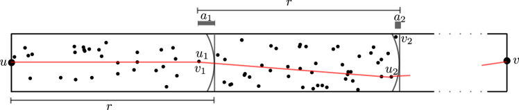
Figure 2. The points $u_{1}$, $v_{1}$ coincide but $u_{2}$ and $v_{2}$ do not

Note that the vertices $u,v_{1},v_{2},\ldots,v_{k}$ may not induce a connected path in $\widetilde{\mathscr{G}}_{u,v}(n,r)$, since the Euclidean distance between two consecutive ones may be greater than $r$. However, the fact that $v_{i}$ is the vertex with largest $x$-coordinate inside $[0,x_{i-1}+r]\times[-\alpha,\alpha]$ and together with a straightforward induction argument yield to the following claim: if $u=u_{0},u_{1},u_{2}\ldots,u_{k}$ is a path contained in $R$, then for every $1\leq i\leq k$ the $x$-coordinate of $u_{i}$ is at most $x_{i}$ (see again Figure 2). We will now show that $x_{k}<t$ with the desired probability.

Define

$$a=\sum_{i=1}^{k}a_{i}\qquad\text{and}\qquad\tilde{a}=\sum_{i=1}^{k}\tilde{a}_{i}.$$

Expanding recursively from the relations $x_{i}=x_{i-1}+r-a_{i}$ and $x_{1}=r-a_{1}$, we get

$$x_{k}=\sum_{i=1}^{k}(r-a_{i})=kr-a.$$

Let us consider the event that $\tilde{a}_{i}\leq r/2$ for all $1\leq i\leq k$. In particular, this event implies that $a_{i}=\tilde{a}_{i}$ for all $i$, and therefore $x_{k}=kr-\tilde{a}$. Since each $\tilde{a}_{i}$ is exponentially distributed with parameter $2\alpha$,

$$\Pr\left(\exists i:a_{i}>r/2\right)\leq k\Pr\left(a_{1}>r/2\right)=ke^{-\alpha r}\;,$$ (5)

so $x_{k}=kr-\tilde{a}$ with probability at least $1-ke^{-\alpha r}$.

Moreover, notice that

$$\mathbb{E}(\tilde{a})=k\mathbb{E}(\tilde{a}_{1})=\frac{k}{2\alpha}\;.$$

By Lemma 2.1, for all $0<\varepsilon<1$,

$$\Pr\left(\tilde{a}\leq(1-\varepsilon)\frac{k}{2\alpha}\right) \leq\left((1-\varepsilon)e^{\varepsilon}\right)^{k}<e^{-\varepsilon^{2}k/2}\;.$$ (6)

where we have used that $\log(1-x)<-x-\frac{x^{2}}{2}$, for any $0<x<1$.

If $t<kr\left(1-\frac{\delta}{(tr)^{2/3}}\right)=kr(1+o(1))$, by definition of $B$, $\Pr(B)=0$ and we are done. Thus, we may assume that $t\geq kr(1+o(1))$. For $\delta=\left(\frac{1-\varepsilon}{\sqrt{2}}\right)^{2/3}$, from (6) and (5),

$$\Pr\left(x_{k}\geq t\right) \leq\Pr\left(x_{k}\geq kr\left(1-\frac{\delta}{(tr)^{2/3}}\right)\right)$$

$$\leq\Pr\left(x_{k}\geq kr-\frac{\sqrt{2}\delta^{3/2}kr}{t}\cdot\frac{k}{2\alpha}\right)$$

$$\leq\Pr\left(x_{k}\geq kr-(1-\varepsilon+o(1))\frac{k}{2\alpha}\right)$$

$$\leq\Pr\left(\exists i:a_{i}>r/2\right)+\Pr\left(\forall i:a_{i}\leq r/2\text{and}a\leq(1-\varepsilon+o(1))\frac{k}{2\alpha}\right)$$

$$\leq\Pr\left(\exists i:a_{i}>r/2\right)+\Pr\left(\tilde{a}\leq(1-\varepsilon+o(1))\frac{k}{2\alpha}\right)$$

$$\leq ke^{-\alpha r}+e^{\varepsilon^{2}k/2}$$

$$\leq\frac{t}{r}\exp\left(-\sqrt{\delta/2}(tr)^{2/3}\right)+\exp\left(-(1-\sqrt{2\delta^{3}})^{2}\frac{t}{2r}\right)\;.$$

Hence, if $A_{\alpha}$ holds, then $\Pr{(B)}\leq\Pr\left(x_{k}\geq t\right)\leq\frac{t}{r}\exp\left(-\sqrt{\delta/2}(tr)^{2/3}\right)+\exp\left(-(1-\sqrt{2\delta^{3}})^{2}\frac{t}{2r}\right)$, and if $\overline{A_{\alpha}}$ holds, then $\Pr{(B)}=0$. Thus, the proposition follows. ∎

Proposition 2.4.

Let $\widetilde{\mathscr{G}}_{u,v}(n,r)$ be a random geometric graph in $\mathcal{S}_{n}$ with labelled vertices $u$ and $v$ such that $d_{E}(u,v)\geq 20r\log{n}$. Then we have

$$d_{G}(u,v)\leq\frac{d_{E}(u,v)}{r}\left(1+\frac{1}{2(rd_{E}(u,v))^{2/3}}\right)\;,$$

with probability at most $o(n^{-5/2})$.

Proof.

As before, let $t=d_{E}(u,v)$ and $k=d_{G}(u,v)$. Also let $\delta=1/2$.

Since $t\geq 20r\log{n}$ and $r\geq r_{c}=\Omega(\sqrt{\log{n}})$, we have

$$\sqrt{\delta/2}(tr)^{2/3}-\log{(t/r)}=\Omega(\log^{4/3}{n})\;,$$

and

$$\left(1-\sqrt{2\delta^{3}}\right)^{2}\frac{t}{2r}\geq\frac{5}{2}\log{n}\;.$$

By Proposition 2.3, this implies that

$$\Pr\left(k\leq\frac{t}{r}\left(1+\frac{1}{2(tr)^{2/3}}\right)\right)=o(n^{-5/2})\;.$$

∎

To finish the proof of statement (i) in Theorem 1.1, by de-Poissonizing $\widetilde{\mathscr{G}}_{u,v}(n,r)$, we have that in $\mathscr{G}(n,r)$, statement (i) in Theorem 1.1 holds for our choice of $u$ and $v$, with probability at least $1-o(n^{-2})$. Note that this fact does not depend on the particular location of $u$ and $v$ in $\mathcal{S}_{n}$. The statement follows by taking a union bound over all at most $n^{2}$ pairs of vertices.

2.2. Proof of statement (ii)

As in Subsection 2.1, we pick two points in $\mathcal{S}_{n}$, and put $t=d_{E}(u,v)$. Let $\gamma$ be as in the statement of Theorem 1.1. We assume first that $u=(0,0)$ and $v=(t,0)$, and consider a Poisson point process in the rectangle $R=[0,t]\times[0,\alpha]$, for a certain $\alpha\leq r$ that will be made precise later.

Let $\widetilde{\mathscr{G}}_{R,u,v}(n,r)$ denote the random geometric graph on the rectangle $R$, to which the points $u$ and $v$ are added. We will show that the probability of having $d_{G}(u,v)\geq\frac{d_{E}(u,v)}{r}\left(1+\delta r^{-4/3}\right)$ decays exponentially in $\delta$. For each point $z$ in $R$ with $x$-coordinate $s$, define the rectangle

$$R_{z}=\left[s,s+\rho\right]\times[0,\alpha],\qquad\text{where}\quad\rho=r-\frac{\alpha^{2}}{r}.$$

We need the following auxiliary lemma.

Lemma 2.5.

For any vertex $z$ in $R$, all vertices in $R_{z}$ are connected to $z$ (see Figure 3).

Proof.

It is enough to show that the upper-left and the bottom-right corner of $R_{z}$ are at distance at most $r$. Then all vertices inside $R_{z}$ are connected to one another, and in particular $z$ is connected to every vertex in $R_{z}$. A sufficient condition for that is

$$\sqrt{\rho^{2}+\alpha^{2}}\leq r,$$

or equivalently

$$r\left(1-(\alpha/r)^{2}\right)=\rho\leq\sqrt{r^{2}-\alpha^{2}}=r\sqrt{1-(\alpha/r)^{2}}.$$

Since $\sqrt{1-x}>1-x$ for any $0<x<1$, the lemma follows. ∎

Figure 3. The rectangle $R_{z}$

Proposition 2.6.

Let $\widetilde{\mathscr{G}}_{R,u,v}(n,r)$ be a random geometric graph on $R$, with $u=(0,0)$ and $v=(t,0)$. Let $F>0$ and $J>\frac{3(F+1)}{2^{2/3}}$ be constants and define $g(x)=x-\log(1+x)$. Then, for every $J\leq\delta\leq Fr^{4/3}$, we have that

$$\Pr\left(d_{G}(u,v)>\left\lceil\frac{t}{r}\left(1+\delta r^{-4/3}\right)\right\rceil\right)\leq n\exp\left(-\frac{(F+1)\delta^{1/2}r^{4/3}}{2J^{3/2}}\right)+\exp\left(-g\Big{(}(\delta/J)^{3/2}\Big{)}\frac{t}{r}\right).$$

Proof.

Set $C=1/J^{3/2}$, and let $B$ be any positive constant satifying

$$B^{2}+C/B\leq 1/(F+1).$$ (7)

Some elementary analysis shows that such $B$ must exist. In fact, the equation $B^{2}+C/B=1/(F+1)$ has exactly two positive solutions $B_{1}$ and $B_{2}$ for any $0<C<\frac{2}{(3(F+1))^{3/2}}$, and any $0<B_{1}\leq B\leq B_{2}<1/\sqrt{F+1}$ satisfies (7).

Let us consider the integer $k=\lceil\frac{t}{r}(1+\delta r^{-4/3})\rceil$. We will show that with very high probability there exists a path length at most $k$ between $u$ and $v$. Such a path will only use vertices inside $R$, but for technical reasons (the last of the rectangles $R^{\prime}_{i}$ defined below might be further to the right than the point $(t,0)$ or possibly be outside of the square) of the argument we extend the Poisson point process of our probability space to the semi-infinite strip $R_{\infty}=[0,\infty)\times[0,\alpha]$.

We construct a sequence of vertices in a similar way as in the proof of Proposition 2.3. Set $v_{0}=u$, $x_{0}=0$ and $a_{0}=0$. We make the choice of $\alpha$ for this subsection now more precise. We set

$$\alpha=B\delta^{1/2}r^{1/3},$$

for some constant $0<B<1/\sqrt{F+1}$ satisfying (7). Observe that the restriction $\delta\leq Fr^{4/3}$ implies that

$$\alpha\leq(B\sqrt{F})r<r,$$ (8)

so our choice of $\alpha$ is feasible, and moreover

$$\rho=r-\alpha^{2}/r\geq(1-B^{2}F)r.$$ (9)

For each $1\leq i\leq k-1$, define $R^{\prime}_{i}=(x_{i-1}+a_{i-1},x_{i-1}+\rho]\times[0,\alpha]$, and let $v_{i}$ be the vertex with largest $x$-coordinate inside $R^{\prime}_{i}$ (if $R^{\prime}_{i}$ is empty, then add an extra vertex $v_{i}=(x_{i-1}+a_{i-1},0)$). Define $x_{i}$ to be the $x$-coordinate of $v_{i}$ and $a_{i}=x_{i-1}+\rho-x_{i}$. By the same considerations as in the proof of Proposition 2.3 (but replacing $R_{i}$ by $R^{\prime}_{i}$, $r$ by $\rho$, and $k$ by $k-1$), we deduce that $a_{1},a_{2},\ldots,a_{k-1}$ are stochastically dominated by a sequence $\tilde{a}_{1},\tilde{a}_{2},\ldots,\tilde{a}_{k-1}$ of i.i.d. exponentially distributed random variables of parameter $\alpha$, such that $a_{i}=\min\{\tilde{a}_{i},\rho-a_{i-1}\}\leq\tilde{a}_{i}$ for all $1\leq i\leq k-1$. Moreover, since $\alpha\rho/2\geq(1-B^{2}F)\alpha r/2=(1-B^{2}F)B\delta^{1/2}r^{4/3}/2$, we have

$$\Pr(\tilde{a}_{i}>\rho/2)=e^{-\alpha\rho/2}\leq e^{-(1-B^{2}F)B\delta^{1/2}r^{4/3}/2}\;.$$

Thus, with probability at least $1-ke^{-(1-B^{2}F)B\delta^{1/2}r^{4/3}/2}$, for every $1\leq i\leq k-1$ we have $\tilde{a}_{i}\leq\rho/2$, and therefore $a_{i}=\tilde{a}_{i}$. This event implies that

$$x_{k-1}=(k-1)\rho-\tilde{a},$$ (10)

where $\tilde{a}=\sum_{i=1}^{k-1}\tilde{a}_{i}$, and also that we did not add any extra vertices (i.e. all $v_{1},\ldots,v_{k-1}$ belong to the Poisson point process in $[0,\infty)\times[0,\alpha]$).

By construction, each $x_{i}$ belongs to the rectangle $R^{\prime}_{i}\subseteq R_{v_{i-1}}$ for every $1\leq i\leq k-1$. Hence, by Lemma 2.5, the vertices $v_{0},v_{1},\ldots,v_{k-1}$ form a connected path.

In view of all that, it suffices to show that $x_{k-1}+\rho\geq t$ with sufficiently large probability. Note that, if this event holds, then $v$ must belong to $R_{v_{j}}$ for some $0\leq j\leq k-1$, and therefore $u=v_{0},v_{1},v_{2}\ldots,v_{j},v$ is a connected path of length $j+1\leq k$. (Observe that such a path is contained in $R$, so our extension of the Poisson point process to $R_{\infty}$ turned out to be harmless.)

Recall that $C=1/J^{3/2}$. Using the upper-tail bound in Lemma 2.1 we obtain

$$\Pr\left(\tilde{a}\geq(1+C\delta^{3/2})\frac{k}{2\alpha}\right)<\left(\frac{1+C\delta^{3/2}}{e^{C\delta^{3/2}}}\right)^{k}\leq e^{-kg\left((\delta/J)^{3/2}\right)}.$$

Combining this together with (10), we infer that, with probability at least

$$1-ke^{-(1-B^{2}F)B\delta^{1/2}r^{4/3}/2}-e^{-kg\left((\delta/J)^{3/2}\right)},$$

we have

$$x_{k-1}+\rho=k\rho-\tilde{a}>k\rho-\frac{\left(1+C\delta^{3/2}\right)k}{2\alpha}=kr\Big{(}1-\frac{\alpha^{2}}{r^{2}}-\frac{(1+C\delta^{3/2})}{2\alpha r}\Big{)}.$$ (11)

From the definition of $k$, the range of $\delta$ and since $\alpha=B\delta^{1/2}r^{1/3}$, the event above implies

$$x_{k-1}+\rho >t(1+\delta r^{-4/3})\bigg{(}1-\delta r^{-4/3}\Big{(}B^{2}+\frac{(\delta^{-3/2}+C)}{2B}\Big{)}\bigg{)}$$

$$\geq t(1+\delta r^{-4/3})\bigg{(}1-\delta r^{-4/3}\Big{(}B^{2}+\frac{C}{B}\Big{)}\bigg{)}$$

$$=t\Bigg{[}1+\delta r^{-4/3}\bigg{(}1-\big{(}\delta r^{-4/3}+1\big{)}\Big{(}B^{2}+\frac{C}{B}\Big{)}\bigg{)}\Bigg{]}$$

$$\geq t\Bigg{[}1+\delta r^{-4/3}\bigg{(}1-(F+1)\Big{(}B^{2}+\frac{C}{B}\Big{)}\bigg{)}\Bigg{]}>t,$$

so

$$\Pr(d_{G}(u,v)>k) \leq ke^{-(1-B^{2}F)B\delta^{1/2}r^{4/3}/2}+e^{-kg\left((\delta/J)^{3/2}\right)}$$

$$\leq ne^{-(1-B^{2}F)B\delta^{1/2}r^{4/3}/2}+e^{-g\left((\delta/J)^{3/2}\right)t/r}$$ (12)

$$\leq ne^{-(1-B^{2}(F+1))B\delta^{1/2}r^{4/3}/2}+e^{-g\left((\delta/J)^{3/2}\right)t/r}$$

$$\leq ne^{-C(F+1)\delta^{1/2}r^{4/3}/2}+e^{-g\left((\delta/J)^{3/2}\right)t/r},$$ (13)

as desired. On the last step we used the fact that $(1-B^{2}(F+1))B\geq C(F+1)$, which easily follows from (7). This completes the proof of the proposition. Note that (12) may be stronger than (13) if we choose a constant $B$ which satisfies (7) and maximises $(1-B^{2}F)B$. ∎

Proposition 2.7.

Let $\gamma$ as in the statement of Theorem 1.1, and let $\widetilde{\mathscr{G}}_{R,u,v}(n,r)$ be a random geometric graph on $R$, with $u=(0,0)$ and $v=(t,0)$. Suppose that $r\geq 70\sqrt{\log n}$. Then we have

$$d_{G}(u,v)>\left\lceil\frac{t}{r}\left(1+70\gamma(rt)^{-2/3}\right)\right\rceil,$$

with probability at most $o(n^{-5/2})$.

Proof.

First, observe that, if $t\leq r$, then $d_{G}(u,v)=1$, and the statement holds trivially. Thus, we assume henceforth that $t>r$.

Set $B=47/50$, $C=10^{-2}$, $F=23/200$, $D=70$, $E=31$ and $J=10^{-4/3}$. Recall that

$$\gamma=\max\left\{E\left(\frac{2r\log{n}}{r+t}\right)^{2/3},D\frac{\log^{2}{n}}{r^{8/3}},3^{2/3}J\right\}\;.$$

We want to apply Proposition 2.6 with $\delta=\gamma$. It is straightforward to check that the restrictions (7) and $J>\frac{3(F+1)}{2^{2/3}}$, required in Proposition 2.6 hold. We also need to show that $J\leq\gamma\leq Fr^{4/3}$. Notice that $\frac{D\log^{2}{n}}{r^{8/3}}\leq Fr^{4/3}$, since $r\geq 70\sqrt{\log{n}}\geq(D/F)^{1/4}\sqrt{\log{n}}$; also $E\left(\frac{2r\log{n}}{r+t}\right)^{2/3}\leq Fr^{4/3}$, since $r(r+t)/(2\log n)>r^{2}/\log n\geq 4900\geq(E/F)^{3/2}$; and finally $3^{2/3}J\leq Fr^{4/3}$ since $r=\Omega(\sqrt{n})$. Moreover, $\delta\geq 3^{2/3}J\geq J$.

Note that this choice of constants combined with (8) and (9) implies

$$\alpha\leq r/3\qquad\text{and}\qquad\rho\geq 8r/9\geq 8\alpha/3.$$ (14)

The proof concludes by applying (12) in the proof of Proposition 2.6 with this given $\delta$, showing that the upper bound on $\Pr(d_{G}(u,v)>k)$ is $o(n^{-5/2})$. On the one hand, $\delta\geq\frac{D\log^{2}{n}}{r^{8/3}}$ implies

$$\frac{(1-B^{2}F)B\delta^{1/2}r^{4/3}}{2}-\log n\geq\frac{(1-B^{2}F)BD^{1/2}\log n}{2}-\log n>\frac{7.01}{2}\log{n}-\log{n}=\frac{5.01}{2}\log{n}.$$

On the other hand, $\delta\geq E(r\log{n}/t)^{2/3}$ and $\delta\geq 3^{2/3}J$ imply

$$\frac{g\left((\delta/J)^{3/2}\right)t}{r}>\frac{(\delta/J)^{3/2}t}{2r}\geq\frac{3}{2}CE^{3/2}\log n>\frac{5.17}{2}\log{n},$$

where we have used that $g(x)\geq x/2$ if $x\geq 3$.

Therefore, $\Pr(d_{G}(u,v)>k)\leq n^{-5.01/2}+n^{-5.17/2}=o(n^{-5/2})$. ∎

Corollary 2.8.

Statement (ii) in Theorem 1.1 is true.

Proof.

Observe that from the proof of Proposition 2.6 together with (14), $x_{1}\geq\rho/2>4\alpha/3$ with probability at least $1-o(n^{-5/2})$. In particular, this event implies that $v_{1}$ is outside of the square $[0,1.01\alpha]\times[0,\alpha]$. Moreover, also with probability $1-o(n^{-5/2})$, we can find some point $\hat{v}_{j}$ in $[t-1.01\alpha-r/2,t-1.01\alpha]\times[0,\alpha]$. It may happen that $v_{j}$ lies in $[t-1.01\alpha,t]\times[0,\alpha]$. However, in that case, we can replace $v_{j}$ with $\hat{v}_{j}$, and therefore we found a $u$–$v$ path of length $j+1\leq k$ with all internal vertices in $[1.01\alpha,t-1.01\alpha]\times[0,\alpha]$. Indeed, we will show now that we can always fit such a rectangle $R^{\prime}=[1.01\alpha,t-1.01\alpha]\times[0,\alpha]$, suitably rotated and translated, into the square. We need first a few definitions.

Consider two points $u=(x_{u},y_{u})$ and $v=(x_{v},y_{v})$ in $\mathbb{R}^{2}$. By symmetry we may assume that $x_{u}<x_{v}$ and $y_{u}\leq y_{v}$. Let $\beta$ be the angle of the vector $\vec{uv}$ with respect to the horizontal axis. Again by symmetry, we may consider $\beta\in[0,\pi/4]$.

We consider now two rectangles of dimensions $\alpha\times t$ placed on each side of the segment $uv$. Let $R^{+}$ be the rectangle to the left of $\vec{uv}$, and let $R^{-}$ be the rectangle to the right of $\vec{uv}$. We will show that at least one of these rectangles contains a copy of $R^{\prime}$ fully contained in $\mathcal{S}_{n}$.

Notice that the intersection of $R^{+}$ and $R^{-}$ with each of the halfplanes $x\leq x_{u}$, $x\geq x_{v}$, $y\leq y_{u}$ and $y\geq y_{v}$ gives $4$ triangles. We call them $T_{u}^{+}$, $T_{v}^{-}$, $T_{u}^{-}$ and $T_{v}^{+}$ respectively. All these triangles are right-angled, and denote by $t_{u}^{+}$, $t_{v}^{-}$, $t_{u}^{-}$ and $t_{v}^{+}$ the side of the corresponding triangle that it is parallel to the segment $uv$. Notice that $|t_{u}^{+}|=|t_{v}^{-}|$ and $|t_{u}^{-}|=|t_{v}^{+}|$. Call a triangle $T_{w}^{*}$, with $w\in\{u,v\}$ and $*\in\{+,-\}$, safe if $|t_{w}^{*}|\leq 1.01\alpha$. Note that if $T_{u}^{+}$ and $T_{v}^{+}$ are safe or fully contained in the square, then $R^{+}$ contains the desired rectangle $R$, and analogously for $R^{-}$.

Since we assumed that $\beta\leq\pi/4$, we have $|t_{u}^{+}|=|t_{v}^{-}|=\alpha|\tan\beta|\leq 1.01\alpha$. Thus, $T_{u}^{+}$ and $T_{v}^{-}$ are safe. If $y_{u}=y_{v}$, that is $\beta=0$, it is clear that either $R^{+}$ or $R^{-}$ contain the desired copy of $R^{\prime}$. Thus, we may assume that $\beta>0$.

We can also assume that both $u$ and $v$ are on the boundary of $\mathcal{S}_{n}$, as otherwise we extend the line segment $uv$ to the boundary of the square, and the original rectangles are contained in the new ones.

Recall that $T_{u}^{+}$ and $T_{v}^{-}$ are safe. If $y_{v}\leq\sqrt{n}/2-\alpha$, then $T_{v}^{+}$ is completely contained in the square, and hence $R^{+}$ satisfies the conditions. Similarly, if $y_{u}\geq-\sqrt{n}/2+\alpha$, $R^{-}$ satisfies the conditions. Otherwise, $|y_{u}|,|y_{v}|\geq\sqrt{n}/2-\alpha$, and the angle $\beta$ is at least $\arctan\left(\frac{\sqrt{n}-2\alpha}{\sqrt{n}}\right)>\pi/4$, which contradicts our assumption on $\beta$.

Again, by de-Poissonizing $\widetilde{\mathscr{G}}_{u,v}(n,r)$, we can use Proposition 2.7 to show that for given $u$ and $v$ in $G\in\mathscr{G}(n,r)$, statement (ii) in Theorem 1.1 holds with probability at least $1-o(n^{-2})$. By taking a union bound over all at most $n^{2}$ possible pairs of vertices, statement (ii) in Theorem 1.1 follows. ∎

3. Open problems

Theorem 1.1 establishes a relation between the graph distance and the Euclidean distance of two vertices $u$ and $v$ in $\mathscr{G}(n,r)$ that holds a.a.s. simultaneously for all pairs of vertices.

It would be interesting to find better concentration bounds on the values that $d_{G}(u,v)$ can take with high probability. Also, we would like to characterize the probability distributions of $\mathbb{E}(d_{G}(u,v)\mid d_{E}(u,v))$ and ${\rm Var}(d_{G}(u,v)\mid d_{E}(u,v))$ (i.e. the expectation and variance of $d_{G}(u,v)$ given $d_{E}(u,v)$). What can we say about these distributions?

In the proof of statement (ii) in Theorem 1.1, we define a new random variable that stochastically dominates $d_{G}(u,v)$ and we give an upper bound for the probability that this random variable is too large. This argument can be easily adapted in the case $r=\omega(r_{c})$, and provide the upper bound $\mathbb{E}(d_{G}(u,v)\mid d_{E}(u,v))-d_{E}(u,v)/r=O\left(1+\gamma d_{E}(u,v)r^{-7/3}\right)$. Similarly, the proof of statement (i) in Theorem 1.1 can be adapted to give a lower bound on $\mathbb{E}(d_{G}(u,v))\mid d_{E}(u,v))$, but we need the further conditioning upon the event that $d_{E}(u,v)$ is large enough.

References

- [1] M. Bradonjic, R. Elsässer, T. Friedrich, T. Sauerwald and A. Stauffer, Efficient broadcast on random geometric graphs. Proceedings of the Twenty-First Annual ACM-SIAM Symposium on Discrete Algorithms, pp. 1412–1421. Society for Industrial and Applied Mathematics, 2010.
- [2] R. B. Ellis, J. L. Martin and C. Yan, Random geometric graph diameter in the unit ball Algorithmica, 47(4), pp. 421–438, 2007.
- [3] E.N. Gilbert, Random Plane Networks, J. Soc. Industrial Applied Mathematics, 9(5), pp. 533–543, 1961.
- [4] A. Goel, S. Rai and B. Krishnamachari, Sharp thresholds for monotone properties in random geometric graphs, Annals of Applied Probability, 15, pp. 364–370, 2005.
- [5] G. Grimmett and D. Stirzaker, Probability and Random Processes (3rd Edition), Oxford U. P., 2001.
- [6] T. Friedrich, T. Sauerwald and A. Stauffer, Diameter and broadcast time of random geometric graphs in arbitrary dimensions, Algorithms and Computation pp. 190–199, Springer Berlin Heidelberg, 2011.
- [7] A. Merhabian and N. Wormald, On the stretch factor of randomly embedded random graphs, http://arxiv.org/pdf/1205.6252v1.pdf, 2013.
- [8] S. Muthukrishnan and G. Pandurangan, The bin-covering technique for thresholding random geometric graph properties, Proceedings of the sixteenth annual ACM-SIAM symposium on Discrete algorithms, pp. 989–998. Society for Industrial and Applied Mathematics, 2005.
- [9] M. Penrose, The longest edge of the random minimal spanning tree, Annals of Applied Probability, 7(2), pp. 340–361, 1997.
- [10] M. Penrose, Random Geometric Graphs, Oxford Studies in Probability. Oxford U.P., 2003.