Appearance of the Single Gyroid Network Phase in Nuclear Pasta Matter

Abstract

Nuclear matter under the conditions of a supernova explosion unfolds into a rich variety of spatially structured phases, called nuclear pasta. We investigate the role of periodic network-like structures with negatively curved interfaces in nuclear pasta structures, by static and dynamic Hartree-Fock simulations in periodic lattices. As the most prominent result, we identify for the first time the single gyroid network structure of cubic chiral $I4_{1}23$ symmetry, a well known configuration in nanostructured soft-matter systems, both as a dynamical state and as a cooled static solution. Single gyroid structures form spontaneously in the course of the dynamical simulations. Most of them are isomeric states. The very small energy differences to the ground state indicate its relevance for structures in nuclear pasta.

I Introduction

Nuclear matter, although not observable in laboratories on earth, plays a crucial role in astrophysical scenarios such as neutron stars or core-collapse supernovae Bethe ; Suzuki . Near equilibrium density, nuclear matter is a homogeneous quantum liquid, somewhat trivial from a structure perspective. However, an exciting world of various geometrical profiles develops at lower densities covering ensembles of rods, slabs, tubes, or bubbles Ravenhall ; Hashimoto ; Pais ; Watanabe2001 ; Schuetrumpf2013a . Most of these phases can be considered as manifestations of liquid crystals Pethick1998 and the geometrical analogy to spaghetti, lasagna etc. has led to summarize these under the notion of a nuclear “pasta”. Their complex shapes and topologies can be classified by integral curvature measures Nakazato2009 ; Nakazato2011 ; Schuetrumpf2013a , developed in the realm of soft matter physics and known as Minkowski functionals Mecke:1998 ; MeckeStoyan:2000 ; SchroederTurketal:2010 ; SchroederTurk:2013 .

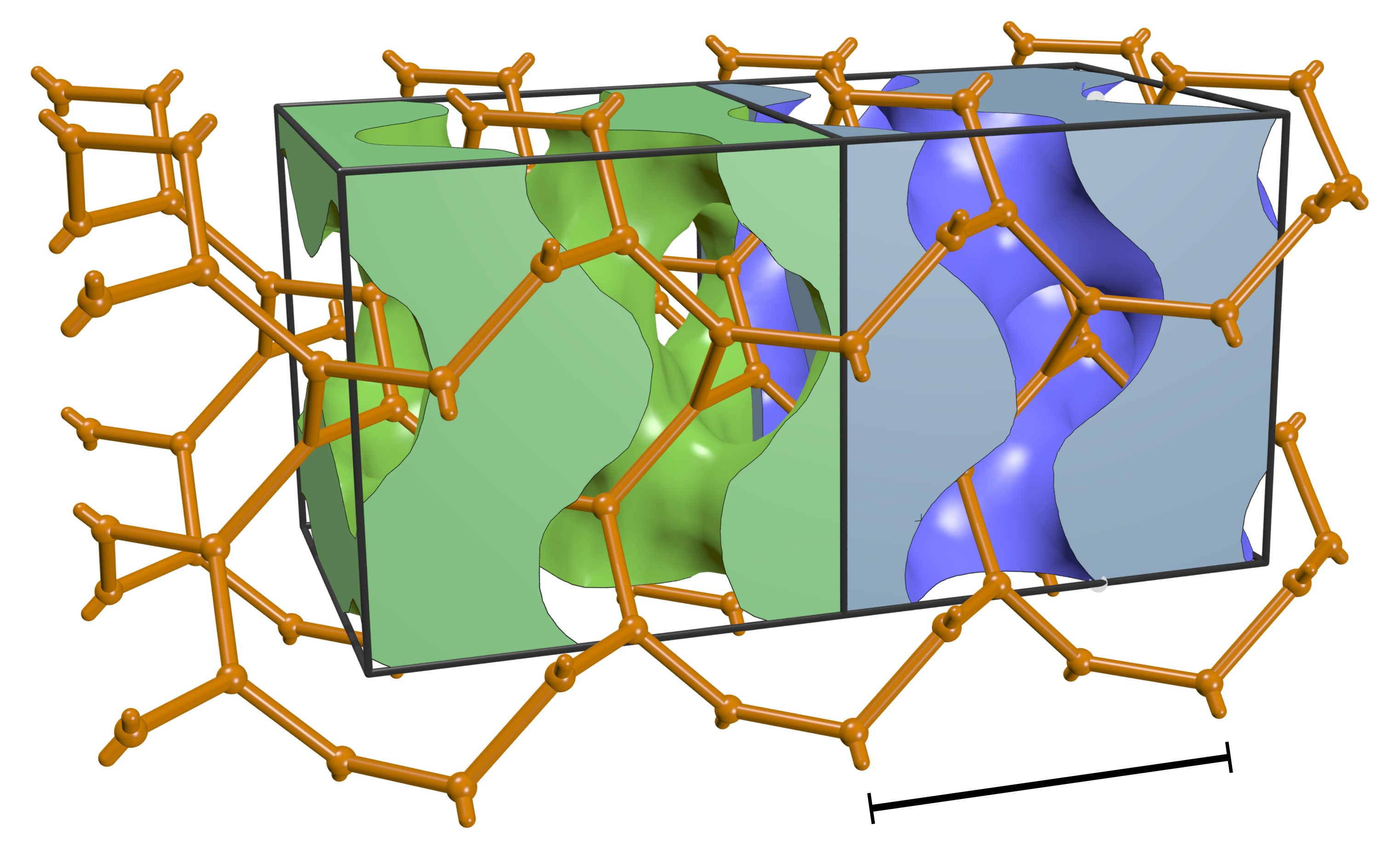
Figure 1: (Color online) Gyroidal pasta shape: the green structure on the left hand represents the density distribution of the gyroidal state of nuclear pasta matter computed with TDHF for an average density of $0.06{\rm\,fm^{-3}}$ and box length $a=22\,\mathrm{fm}$. Shown is the Gibbs dividing surface with a corresponding threshold density. The solid volume representing densities above this value and the void representing densities below this value. The blue structure on the right hand side shows the nodal approximation (4) of a single gyroid CMC surface at the same volume fraction. Also shown by orange bars is a gyroid network in the void phase of both the pasta shape and the nodal approximation, showing that they are indeed homotopic. Black frames are guides to the eye, of size $1.25\,a$ the cubic lattice parameter.

A particularly intricate structure amongst the pasta phases is the gyroid, a triply-periodic geometry consisting of two inter-grown network domains separated by a periodic manifold-like surface which is (at least on average) saddle-shaped and with negative Gaussian curvature (cf. Fig. 1). In soft-matter systems, these periodic saddle-shaped surfaces have been found in solid biological systems MichielsenStavenga:2008 ; SaranathanOsujiMochrieNohNarayananSandyDufresnePrum:2010 ; SchroederTurkWickhamAverdunkBrinkFitzGeraldPoladianLargeHyde:2011 ; GalushaRicheyGardnerChaBartler:2008 ; Pouya:11 ; Wilts2012 ; Nissen:1969 , in the so-called ’core-shell’ gyroid phase of di-block copolymers HajdukHarperGrunerHonekerKimThomasFetters:1994 and in inverse bicontinuous phases in lipid-water systems Larsson:1989 . Gyroid-like geometries can also be expected in nuclear pasta, due to a balance between the nuclear and Coulomb forces Nakazato2009 ; Nakazato2011 . Similar kinds of periodic bicontinuous structures are discussed in supernova cores and neutron star crusts Pethick ; Mat06a . It is generally accepted that liquid crystalline phases, i.e., pasta phases, occur in supernova cores in the form of slabs, rods and tubes Ravenhall ; Hashimoto ; Pais ; Watanabe2001 . The search for elaborate structures in astro-physical matter with self-consistent nuclear models has a long history, starting from the first full Skyrme-Hartree-Fock (SHF) simulation of Bonche . With continued refinement of the calculations, more and more intricate structures had been discovered. For example, the possible occurrence of periodic bicontinuous structures was found by stationary Hartree-Fock calculations Goe01aR ; Mag02 ; Goe07a ; NewtonStone ; Pais , later on in dynamical simulations of supernova matter using time-dependent Hartree-Fock (TDHF) calculations for supernova matter Sebille ; Sebille2011 and also in a quantum molecular dynamics approach Sonoda2008 . Gyroids were examined so far only within a liquid-drop model Nakazato2009 ; Nakazato2011 where double gyroids were found to be energetically close to the ground state. (Note the important difference between single and double Gyroid geometries, see Fig. 2.) If realized in supernova matter, the network-like percolating nature of the gyroid could greatly affect neutrino transport during the collapse of a massive star’s core and the subsequent core bounce. It is the aim of this paper to investigate gyroid structures on the basis of fully quantum-mechanical Hartree-Fock and TDHF simulations. To that end, we employ the well established Skyrme-Hartree-Fock (SHF) energy functional which provides a reliable description of nuclei and nuclear dynamics over the entire nuclear landscape Bender03 and also in astro-physical systems Stone2007 .

Figure 1 provides a graphical demonstration of the key result of this article, namely the occurrence of a meta-stable gyroid phase in nuclear pasta. It shows the Gibbs diving surface (see section II) and draws the liquid phase as filled, the gas phase as void (although in practice filled with some neutron dust). The network-like domain on the left-hand side of the figure represents the liquid (or high density) domain in full SHF calculations whose shape and topology match closely those of one of the gyroid network domains (shown on the left hand side of the figure). The remaining void space (the gas phase) forms a complementary network-like domain with the same topology, albeit of different volume fraction.

II Constant mean-curvature (CMC) surfaces

A quantitative description and identification of the domain shapes in nuclear pasta matter is afforded by the so-called Minkowski functionals, that are here evaluated for the isodensity surfaces of the nuclear density field $\rho(\mathbf{r})$. We first deduce a surface from the given density which divides the space into a liquid phase (solid), and a gas phase (void). To that end, we use the Gibbs dividing surface (a specific isodensity surface), a standard tool of solid state physics Shchukin , which is chosen such that the liquid phase volume $V_{b}$ contains all the matter in a liquid phase with constant density $\rho_{0}$. This means that $V_{b}\rho_{0}=N_{\mathrm{tot}}$ where $N_{\mathrm{tot}}$ is the total number of particles in the box. For $\rho_{0}$ we take the maximum density of the individual states. The fraction $u$ of liquid volume is

$$u=\frac{V_{b}}{V}=\frac{\rho}{\rho_{0}}\;,\;\rho=\frac{N_{\mathrm{tot}}}{V}$$ (1)

where $\rho$ is the mean density and $V$ the volume of the whole numerical box.

Having defined a surface, we can compute the Minkowski functionals which in three dimensions are the volume $V_{b}$, the surface area $A$, the integrated mean curvature $\int H{\rm\,d}A$, and the Euler characteristic $\chi=1/(4\pi)\int{K}{\rm\,d}A$ Schuetrumpf2013a , a topological constant only taking integer values bibfootnote . Mean curvature and $\chi$ are computed the following way: each point on a surface in 3-space has two principal curvatures $\kappa_{1}$ and $\kappa_{2}$; these are used to compose the mean curvature as $H=(\kappa_{1}+\kappa_{2})/2$ and the Gaussian curvature as $K=\kappa_{1}\kappa_{2}$. Negative values of $\chi$ indicate network-like structures Evans2013 . We are interested in what is called hyperbolic surfaces, where the interface is saddle-shaped and has Gaussian curvature $K\leq 0$ ($\kappa_{1}$ and $\kappa_{2}$ with different sign). Such interfaces can form the continuous bounding surfaces of periodic labyrinth-like domains; they now have a firm place in the taxonomy of soft-matter nanostructures HydeLanguageOfShape:1997 . More specifically, we search within the class of constant-mean-curvature surfaces (CMC) which have constant $H$. They provide structures with the same topology and symmetries, yet with variable volume fractions $u(H)$ GrosseBrauckmann1997 ; GrosseBrauckmann1997b ; AndersonEtAl1987 . Gyroids belong to the CMC and require, in particular, that $\chi=-4$.

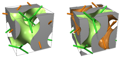
Figure 2: (Color online) Distinction between the single gyroid (left) and double gyroid (right) geometries. The single gyroid consists of a single solid domain (gray) and a single void domain, separated by CMC Gyroid surface. The double gyroid consists in a solid domain (gray) represented by a sheet of finite width draped onto the Gyroid minimal surface and two distinct void domains, each forming a network-like labyrinth. The interfaces between the solid and the void domain in the double Gyroid are two distinct surfaces (brown and green), modelled e.g. by CMC surfaces with constant curvatures $\pm h_{0}$. A second form of the double gyroid, where solid and void is interchanged, also exists. (images from Ref. Kapfer:2011-biomat )

In soft-matter systems, these periodic saddle-shaped surfaces occur in two forms, called “single” or “double”, see Fig.2. The double gyroid (DG) is a structure composed of two inter-grown non-overlapping network domains, bounded by two CMC gyroid surfaces with mean curvatures $\pm H$ separated by the so-called matrix phase. The single gyroid (SG, or simply G) is composed of two domains, one solid and one void of volume fractions $u$ and $(1-u)$, with a gyroid CMC surface as the interface between them; SG have been identified so far only in solid biological systems MichielsenStavenga:2008 ; SaranathanOsujiMochrieNohNarayananSandyDufresnePrum:2010 ; SchroederTurkWickhamAverdunkBrinkFitzGeraldPoladianLargeHyde:2011 ; GalushaRicheyGardnerChaBartler:2008 ; Pouya:11 ; Wilts2012 ; Nissen:1969 . We concentrate in the following on the “single” structures, because double structures were not found to be stable for the assumed parameters in this work.

However, G is not the only CMC structure meeting all of the above criteria. They come along with the related primitive (P) and diamond (D) structures which all three are distinguished by their structural uniformity or homogeneity Hyde:1990 . While any negatively curved interface necessarily exhibits spatial variations of the point-wise Gaussian curvature $K$ (see Ref. Evans:2014 for a discussion) and the point-wise domain width or thickness $d$, the P, D and G surfaces appear to be optimal structures with minimal variations of $K$ FogdenHyde:1999 , and the G surface is the optimal structure with minimal variations of domain width $d$ SchroederFogdenHyde:2006 ; SchroederRamsdenChristyHyde:2003 . This homogeneity is likely to explain the ubiquity of these three structures in soft-matter systems, particularly that of the G. The close relationship between the P, D and G is also visible from the fact that they can be connected by the Bonnet transformation HydeLanguageOfShape:1997 which leaves all metric and curvature properties unchanged and which relates the corresponding unit cell box lengths as $a_{P}/a_{G}=0.81$ and $a_{D}/a_{G}=1.27$. (These ratios correspond to the oriented space groups for the single structures with symmetry groups $Pm\bar{3}m$, $Fd\bar{3}m$, and $I4_{1}32$ for the P, D, and G structures.) While it is not a physical transformation (as intermediate structures are self-intersecting and not embedded), the specific ’Bonnet ratio’ of lattice parameters as given above is often observed in lipid systems that form two of the P, D and G mesophases BaroisHydeNinhamDowling:1990 . This Bonnet ratio can also help to relate and characterize structures. The D surfaces are not found to be stable and thus ignored here.

Table 1: Surface area $A$ and mean curvature $H$ of the exact CMC and pasta P and G surfaces for different mean densities $\rho$ and corresponding volume fractions $u$. For the pasta shapes the average mean curvature $\int H{\rm\,d}A/A$ is given. The values $t_{P}$ and $t_{G}$ are the threshold values for the nodal representations of P and G in Eqs. (3) and (4) with volume fractions $u$. The unit of length is the lattice constant.

		Primitive					Gyroid
$\rho[{\rm\,fm^{-3}}]$	$u$	$A_{P}$		$H_{P}$		$t_{P}$	$A_{G}$		$H_{G}$		$t_{G}$
		CMC	pasta	CMC	pasta		CMC	pasta	CMC	pasta
$0.0326$	$0.22$					$0.99$	$2.61$	$2.84$	$1.96$	$1.85$	$0.86$
$0.0434$	$0.29$	$2.11$		$1.22$		$0.75$	$2.83$	$3.01$	$1.31$	$1.31$	$0.66$
$0.0543$	$0.37$	$2.26$	$2.46$	$0.66$	$0.60$	$0.46$	$3.00$	$3.25$	$0.74$	$0.75$	$0.41$
$0.0651$	$0.45$	$2.33$	$2.51$	$0.24$	$0.23$	$0.18$	$3.08$	$3.34$	$0.28$	$0.26$	$0.16$
$0.0715$	$0.50$	$2.35$		$0.0$		$0.0$	$3.09$		$0.0$		$0.0$
$0.0759$	$0.53$	$2.34$	$2.54$	$-0.13$	$-0.17$	$-0.09$	$3.09$	$3.35$	$-0.15$	$-0.24$	$-0.08$
$0.0868$	$0.61$	$2.29$	$2.44$	$-0.55$	$-0.55$	$-0.39$	$3.02$	$3.30$	$-0.62$	$-0.72$	$-0.34$
$0.0977$	$0.70$	$2.15$		$-1.08$		$-0.69$	$2.87$	$3.10$	$-1.19$	$-1.32$	$-0.60$

Tab. 1 shows values for surface area $A$, volume fraction $u$ and mean curvature $H$ for the G and P surface. One can represent the various surfaces by the simple nodal approximation NesperSchnering1991 in terms of “potential” functions $\phi_{i}(x,y,z)$ with $i\in\{{\rm S,P,G}\}$. For structures scaled to lattice parameters $a=2\pi$ one uses

$$\phi_{S}/\phi_{0} = \cos x\quad,$$ (2)

$$\phi_{P}/\phi_{0} = \cos x+\cos y+\cos z\quad,$$ (3)

$$\phi_{G}/\phi_{0} = \cos x\sin y+\cos y\sin z+\cos z\sin x\quad,$$ (4)

where $\phi_{0}$ is some constant potential value. The slab (S) is generated by the potential (2) producing parallel sheets of matter, also called “lasagna”. The P surface from potential (3) consists in a simple cubic lattice of rods in three orthogonal directions which have common crossing points. The G surface is produced by Eq. (4). The minimal surfaces are approximated by $\phi_{i}(x,y,z)=0$ and the CMC surfaces by $\phi_{i}(x,y,z)/\phi_{0}=\pm t$ (where $t$ is the threshold value for the nodal representation, see table 1). For the volume fractions considered here, the differences between the nodal approximations and the exact CMC surfaces are negligible compared to the spatial resolution of the computational grid.

III Summary of numerical simulation scheme

Here we use nuclear (TD)HF calculations employing the Skyrme energy-density functional, for a review see Ref. Bender03 . To maintain consistency with our previous study Schuetrumpf2013a , we use the parametrization SLy6 Chabanat and consider the proton fraction $X_{p}=1/3$ throughout. The calculations are performed on an equidistant grid in 3D coordinate space. Box size and lattice spacing are adjusted to give the desired conditions of matter. We consider grid spacings of $0.875{\rm\,fm}\leq\Delta r\leq 1.125{\rm\,fm}$ with $N_{x}=N_{y}=N_{z}$ grid points ranging from 16 to 24. This spans periodic simulation boxes in the range $a=15-26{\rm\,fm}$.

Static HF solutions are computed by accelerated gradient iteration Rei82n while time stepping is done with Taylor expansion of the mean-field time-evolution operator, for technical details see Mar14a . We use the Coulomb solver with periodic boundary conditions. Charge neutrality is enforced by assuming a compensating homogeneous cloud of negative charges. This approximation ignores electron screening. Its effect on matter under astro-physical conditions have been much discussed in the past Mar05a ; Watanabe2003a ; Dorso2012 ; Alcain . Although screening lengths vary widely and reach occasionally the order of structure size, the net effect of electron screening is found to be small Mar05a ; Watanabe2003a , thus excusing the homogeneous approximation for the present exploration.

The search for locally stable CMC configurations is done by biased initialization. First, we initialize the system with plane waves up to the wanted amount of protons and neutrons. For the first 1000 static iterations, we imprint a bias by adding an external guiding potential $\phi_{i}$ according to Eqs. (2)-(4) with $\phi_{0}=10{\rm\,MeV}$. After these first 1000 iterations, we switch off the guiding potential and continue with 9000 further pure HF iterations. The system is then driving to a local minimum, not necessarily the ground state. If the stationary state thus found stays close to the intended structure, we consider this structure as (meta)stable.

The dynamical TDHF simulations are initialized similar as in Ref. Schuetrumpf2013a . We take ground-state wavefunctions of $\alpha$-particles and place them randomly in space. As we are simulating at proton fraction $X_{p}=1/3$ only half of the neutrons can packed in these $\alpha$-particles. The remaining neutrons are added as plane waves filling the states with lowest kinetic energy. After all, the set of wavefunctions is ortho-normalized. In contrast to Schuetrumpf2013a , the $\alpha$-particles were taken at rest and the minimal distance between them was larger such that the distribution is more homogeneous (yet still random) and less energetic. Nonetheless, this initialization scheme produces systems at rather large excitation energies with temperature $T\approx 7{\rm\,MeV}$. The mean density was fixed to $\rho=0.06{\rm\,fm^{-3}}$. The box length was varied here in the range $a=20-24{\rm\,fm}$. For each $a$, ten simulations were performed running over $1000\,{\rm fm/c}$. The final structure emerges typically after $400\,{\rm fm/c}$ and then stays stable, of course, as a fluctuating state.

A word is in order about the analysis of sub-structures of infinite systems in a finite simulation box. It is known that the thus imposed periodic boundary conditions have an impact on the structures due to possible symmetry violation by the box and subsequent spatial mismatch Hoc81aB ; All87 ; Oka12a . A study within classical molecular dynamics without Coulomb interactions implies that this may be particularly critical for extended, inhomogeneous structures Gimenez . Spurious shell effects may further blur the analysis in a quantum-mechanical framwork NewtonStone . However, the numerical expense of fully quantum-dynamical simulations sets limits on the affordable box sizes. To get some idea on the size dependence, we vary here the box in the rather broad range 16–26 fm. This average smooths some artifacts and thus allow even more rigorous structure identification. And yet, our calculations are to be viewed as providing indicators of the appearance of the single gyroid. It motivates us to plan much larger calculations which, however, will run on a long time scale.

IV Stationary structures

First, we discuss results from static HF calculations under various conditions of density and box size. The simulation of Ref. Schuetrumpf2013a used only boxes with a box length of $a=16{\rm\,fm}$. The most involved structure found there is topologically identical to a P surface. Here we investigate larger systems up to $a=26{\rm\,fm}$, all at the same proton fraction $X_{P}={1}/{3}$.

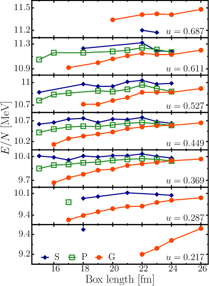
Figure 3: (Color online) Binding energies per nucleon $E/N$ for the metastable ground states for different volume fractions. G (gyroid, dots), P (primitive, squares) and S (slab, diamonds) denotes the initial guiding potential. The states shown in this plot remained topologically stable for the 9000 iterations. Higher values of $E/N$ correspond to more tightly bound and hence more favorable solutions.

We found stable S, P and G structures, the latter both of “single” type. The resulting energies are summarized in Fig. 3. The G is stable for $a\geq 22{\rm\,fm}$ in the widest range of volume fractions compared to P and S. Binding energies of P and G show a clear scaling with box length. For P, the binding energy has a maximum at $a\approx 22{\rm\,fm}$. Under the assumption that an effective description of the pasta Hamiltonian by curvature terms is possible, we expect that the G has a maximum binding energy at $a\approx 27{\rm\,fm}$ due to the Bonnet transformation. The binding energies for P at $a=22{\rm\,fm}$ and G at $a=26{\rm\,fm}$ are lower (and hence less favorable) than for S, except for $u=0.687$, but at this high volume fraction the rod(2) bubble shape (not shown here) has larger binding energies than both G and S. Note that the DG, whose energy was calculated in the liquid drop model Nakazato2009 ; Nakazato2011 , is unstable in the TDHF simulations.

Table 1 shows that surface area $A$ and mean curvature $H$ of the pasta G and P surfaces agree with the exact values, within the rough voxelization of the TDHF calculations. We note a slight but systematic deviation of G and P obtained in TDHF from the nodal models: an anisotropic deformation of the interface surface. While the nodal surface models have cubic symmetry, the directional distribution of interfaces in TDHF are slightly biased towards an axis, exposing more interfacial area in this direction that in the two perpendicular ones. This can be quantified by Minkowski tensor shape analysis, as detailed in SchroederTurketal:2010 ; SchroederTurk:2013 . The eigenvalue ratio $\beta_{1}^{0,2}$ of the interface tensor $W_{1}^{0,2}$ (as defined in SchroederTurk:2013 ), evaluated for a Marching cubes representation of the Gibbs Dividing surface interface, adopts values not below 0.75 for G and values between 0.4 and 1 for P structures.

V Dynamical stability

In order to check dynamical formation and stability of the structures, we performed TDHF simulations and use rather large excitation energies ($T\approx 7{\rm\,MeV}$) which provide a critical counter-check.

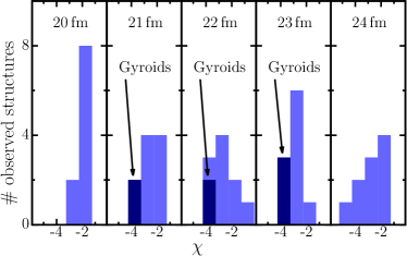
Figure 4: (Color online) Histograms of the resulting Euler characteristic $\chi$ for different box lengths $20-24{\rm\,fm}$ of the dynamic, randomly initialized calculations. The shaded area marks the identified gyroidal structures.

Figure 4 shows the histograms of the Euler characteristic $\chi$ for all box lengths. All structures have negative Euler characteristic, implying that these are labyrinth-like structures: $\chi=-2$ indicates P, $\chi=-3$ corresponds to mixed structures not discussed here, $\chi=-4$ is a necessary condition for G. We finally identify a G by trying to draw the G nodal network through the void. If this turns out to be possible, we have successfully found a single G structure. We have marked it explicitly by shaded areas in figure 4. The figure demonstrates that a great variety of CMC structures can emerge spontaneously in a finite temperature calculation. We note in particular the repeated appearance of the involved, labyrinth-like single gyroid (G) which thus shows that it can be stable even under the extreme conditions of hight temperature. As quantum shell effects disappear at temperatures $T>2$ MeV Bra81a , we also can conclude that the appearance of a G structure is not determined by shell effects (may it be physical or spurious ones NewtonStone ). Note that 10 random samples per box do not provide sufficient statistics to compare quantitatively the abundances of structures. The figure merely indicates their possible appearance even under these highly excited conditions.

The dynamical simulations thus have delivered a couple of (highly excited) G structures. It is interesting to recover stationary G starting static HF from the dynamical states. To that end, we take final states of a TDHF simulation as initial states for a SHF ground state iteration. Doing this for the dynamical G configurations, three cases out of seven remain gyroidal. The binding energies of the cooled gyroidal structure are close to those from purely static calculations. E.g., for $a=22{\rm\,fm}$ we find $E/N=10.357{\rm\,MeV}$ from cooling the dynamical state versus $E/N=10.377{\rm\,MeV}$ from purely static HF. However, the “cooled” dynamical G is more anisotropic (as seen from the tensorial Minkowski measures) while its scalar Minkowski converge to those of the statically calculated G. The binding energy thus depends primarily on the scalar measures like surface area, curvature, and bulk volume and is rather insensitive to the deformation. We thus are probably dealing with a variety of isomeric G configurations. This is another interesting detail calling for further investigations.

VI Conclusions

We have investigated the appearance of non-homogeneous structures in nuclear matter under astro-physical conditions, paying particular attention to structures with network-like geometry and topology, amongst them as particularly appealing shape the single Gyroid (G). To that end, we used static optimization as well as dynamical simulations within a self-consistent nuclear mean-field model (Skyrme-Hartree-Fock). The emerging structures have been characterized by Minkowski measures. To uniquely identify a G, an additional subsequent graphical analysis has been performed. We have shown that single gyroid (G) structures indeed emerge in static and dynamical simulations. We have looked at further CMC surfaces and find close competition with the primitive (P) surface and the slab (S) while the diamond seem to play no role. The static calculations show that G and P are mostly metastable while the S usually provides the ground state, however, with only slightly larger binding energies. G and P, being triply periodic saddle surfaces, have maxima for the binding energies as function of box length, for P at $a\approx 22{\rm\,fm}$ and for G predicted at $a\approx 27{\rm\,fm}$, assuming that the Bonnet transformation is applicable in this system. Dynamical simulations at high excitation energy produce several cases where these structures appear again. This indicates that these network-like geometries are rather robust in nuclear matter. We also find some static G structures with deformations which may be due to the fact that the surface energy is rather small under the given conditions thus easily allowing deformed G isomers.

The large expense of these microscopic calculations limits presently the size of the affordable numerical box. This inhibits so far a unambiguous assessment by studying the trends with box size in larger ranges. The present results are, however, strong indicators for the appearance of CMC and particularly G structures which call for further studies.

- (1) H. A. Bethe, Rev. Mod. Phys. 62, 801 (1990)
- (2) H. Suzuki, Physics and Astrophysics of Neutrinos (Springer, Tokyo, 1994)
- (3) D. G. Ravenhall, C. J. Pethick, and J. R. Wilson, Phys. Rev. Lett. 50, 2066 (1983)
- (4) M. Hashimoto, H. Seki, and M. Yamada, Prog. Theor. Phys. 71, 320 (1984)
- (5) H. Pais and J. R. Stone, Phys. Rev. Lett. 109, 151101 (2012)
- (6) G. Watanabe, K. Iida, and K. Sato, Nucl. Phys. A 687, 512 (2001), ISSN 0375-9474, erratum ibid. 726, 357 (2003)
- (7) B. Schuetrumpf, M. A. Klatt, K. Iida, J. A. Maruhn, K. Mecke, and P.-G. Reinhard, Phys. Rev. C 87, 055805 (2013)
- (8) C. Pethick and A. Potekhin, Phys. Lett. B 427, 7 (1998), ISSN 0370-2693
- (9) K. Nakazato, K. Oyamatsu, and S. Yamada, Phys. Rev. Lett. 103, 132501 (2009)
- (10) K. Nakazato, K. Iida, and K. Oyamatsu, Phys. Rev. C 83, 065811 (2011)
- (11) K. Mecke, Int. J. Mod. Phys. B 12, 861 (1998)
- (12) K. Mecke and D. Stoyan, Statistical Physics and Spatial Statistics - The Art of Analyzing and Modeling Spatial Structures and Pattern Formation, 1st ed., Lecture Notes in Physics, Vol. 554 (Springer, 2000)
- (13) G. E. Schröder-Turk et al., Adv. Mater. 23, 2535 (2011), ISSN 1521-4095
- (14) G. E. Schröder-Turk, W. Mickel, S. C. Kapfer, F. M. Schaller, B. Breidenbach, D. Hug, and K. Mecke, New Journal of Physics 15, 083028 (2013)
- (15) K. Michielsen and D. Stavenga, J. R. Soc. Interface 5, 85 (2008)
- (16) V. Saranathan, C. Osuji, S. Mochrie, H. Noh, S. Narayanan, A. Sandy, E. Dufresne, and R. Prum, PNAS 107, 11676 (2010)
- (17) G. Schröder-Turk, S. Wickham, H. Averdunk, M. Large, L. Poladian, F. Brink, J. Fitz Gerald, and S. T. Hyde, J. Struct. Biol. 174, 290 (2011)
- (18) J. W. Galusha, L. R. Richey, J. S. Gardner, J. N. Cha, and M. H. Bartl, Phys. Rev. E 77, 050904 (2008)
- (19) C. Pouya, D. G. Stavenga, and P. Vukusic, Opt. Express 19, 11355 (2011)
- (20) B. D. Wilts, K. Michielsen, J. Kuipers, H. De Raedt, and D. G. Stavenga, Proc. R. Soc. B(2012), doi:“bibinfo–doi˝–10.1098/rspb.2011.2651˝
- (21) H. Nissen, Science 166, 1150 (1969)
- (22) D. Hajduk, P. Harper, S. Gruner, C. Honeker, G. Kim, E. Thomas, and L. Fetters, Macromolecules 27, 4063 (1994)
- (23) K. Larsson, J. Phys. Chem. 93, 7304 (1989)
- (24) C. J. Pethick and D. G. Ravenhall, Ann. Rev. Nucl. Part. Sci 45, 429 (1995)
- (25) M. Matsuzaki, Phys. Rev. C 73, 028801 (2006)
- (26) P. Bonche and D. Vautherin, Nucl. Phys. A 372, 496 (1981), ISSN 0375-9474
- (27) P. Gögelein, Prog. Part. Nuc. Phys. 59, 206 (2007)
- (28) P. Magierski and P.-H. Heenen, Phys. Rev. C 65, 045804 (2002)
- (29) P. Gögelein and H. Müther, Phys. Rev. C 76, 024312 (2007)
- (30) W. G. Newton and J. R. Stone, Phys. Rev. C 79, 055801 (2009)
- (31) F. Sébille, S. Figerou, and V. de la Mota, Nucl. Phys. A 822, 51 (2009), ISSN 0375-9474
- (32) F. Sébille, V. de la Mota, and S. Figerou, Phys. Rev. C 84, 055801 (2011)
- (33) H. Sonoda, G. Watanabe, K. Sato, K. Yasuoka, and T. Ebisuzaki, Phys. Rev. C 77, 035806 (2008)
- (34) M. Bender, P.-H. Heenen, and P.-G. Reinhard, Rev. Mod. Phys. 75, 121 (2003)
- (35) J. Stone and P.-G. Reinhard, Prog. Part. Nucl. Phys. 58, 587 (2007)
- (36) E. D. Shchukin, A. V. Pertsov, E. A. Amelina, and A. S. Zelenev, Colloid and Surface Chemistry (Elsevier Science B.V., 2001)
- (37) The Euler characteristic is a fundamental morphological descriptor of the topology and connectivity of spatial structure. The Euler characteristic is defined by integral geometry Santalo:1976 ; ArnsKnackstedtPinczewskiMecke:2001 . For a three-dimensional solid body it is given by where is the number of connected components of , the number of handles and the number of hollow cavities (holes) in Santalo:1976 . It is hence a topological quantity (i.e. remains constant if the body is deformed unless the deformation includes cutting or gluing). The Gauss-Bonnet theorem DoCarmo:1976 states that is also given by the integral of the Gaussian curvature over bounding surface , that is . It is important to accurately state if one computes the Euler characteristic of the body or the Euler characteristic of its bounding surface . For a three-dimensional solid body the relation holds. (From Ref. Mickel:2008 ) The Euler characteristic of an orientable surface is related to its genus via .
- (38) M. E. Evans, A. M. Kraynik, D. A. Reinelt, K. Mecke, and G. E. Schröder-Turk, Phys. Rev. Lett. 111, 138301 (2013)
- (39) S. T. Hyde, S. Andersson, K. Larsson, Z. Blum, T. Landh, S. Lidin, and B. Ninham, The Language of Shape, 1st ed. (Elsevier Science, Amsterdam, 1997)
- (40) K. Grosse-Brauckmann, J. Coll. Interf. Sci. 187, 418 (1997), ISSN 0021-9797
- (41) K. Grosse-Brauckmann, Exp. Math. 6, 33 (1997)
- (42) D. Anderson, H. Davis, J. Nitsche, and L. Scriven, in Physics of Amphiphilic Layers, Springer Proceedings in Physics, Vol. 21, edited by J. Meunier, D. Langevin, and N. Boccara (Springer Berlin Heidelberg, 1987) pp. 130–130
- (43) S. C. Kapfer, S. T. Hyde, K. Mecke, C. H. Arns, and G. E. Schröder-Turk, Biomaterials 32, 6875 (2011), ISSN 0142-9612
- (44) S. T. Hyde, in Colloque de Physique C7-1990, Supplément au Journal de Physique (1990) pp. 209–228
- (45) M. E. Evans and G. E. Schröder-Turk, In a Material World. Hyperbolische Geometrie in biologischen Materialien, Mitteilungen der Deutschen Mathematiker Vereinigung, Vol. 22 (de Gruyter, 2014) pp. 158 – 166
- (46) A. Fogden and S. T. Hyde, Eur. Phys. J B 7, 91 (1999)
- (47) G. E. Schröder-Turk, A. Fogden, and S. T. Hyde, Eur. Phys. J B 54, 509 (2006)
- (48) G. E. Schröder, S. Ramsden, A. Christy, and S. T. Hyde, Eur. Phys. J B 35, 551 (2003)
- (49) P. Barois, S. T. Hyde, B. Ninham, and T. Dowling, Langmuir 6, 1136 (1990)
- (50) H. Schnering and R. Nesper, Z. Phys. B 83, 407 (1991), ISSN 0722-3277
- (51) E. Chabanat et al., Nucl. Phys. A 635, 231 (1998), ISSN 0375-9474
- (52) P.-G. Reinhard and R. Cusson, Nucl. Phys. A 378, 418 (1982)
- (53) J. A. Maruhn, P.-G. Reinhard, P. D. Stevenson, and A. S. Umar, Comp. Phys. Comm. to appear (2014), arXiv:1310.5946
- (54) T. Maruyama, T. Tatsumi, D. N. Voskresensky, T. Tanigawa, and S. Chiba, Phys. Rev. C 72, 015802 (2005)
- (55) G. Watanabe and K. Iida, Phys. Rev. C 68, 045801 (2003)
- (56) C. O. Dorso, P. A. P. A. Giménez Molinelli, J. A. López, and E. Ramírez-Homs, “Coulomb forces in neutron star crusts,” ArXiv:1208.4841v1
- (57) P. N. Alcain, P. A. Giménez Molinelli, J. I. Nichols, and C. O. Dorso, Phys. Rev. C 89, 055801 (2014)
- (58) R. Hockney and J. Eastwood, Computer Simulations Using Particles (McGraw-Hill, New York, 1981)
- (59) M. P. Allen and D. J. Tildesley, Computer Simulation of Liquids (Oxford University Press, New York, 1987)
- (60) M. Okamoto, T. Maruyama, K. Yabana, and T. Tatsumi, Phys. Lett. B 713, 284 (2012)
- (61) P. G. Molinelli, J. Nichols, J. López, and C. Dorso, Nuclear Physics A 923, 31 (2014), ISSN 0375-9474
- (62) M. Brack and P. Quentin, Nucl. Phys. A 361, 35 (1981)
- (63) L. A. Santaló, Integral Geometry and Geometric Probability (Addison-Wesley, 1976)
- (64) C. H. Arns, M. A. Knackstedt, W. V. Pinczewski, and K. R. Mecke, Phys. Rev. E 63, 031112 (2001)
- (65) M. Do Carmo, Differential Geometry of Curves and Surfaces (Prentice Hall, Englewood Cliffs, NJ, 1976)
- (66) W. Mickel, S. Münster, L. M. Jawerth, D. A. Vader, D. A. Weitz, A. P. Sheppard, K. Mecke, B. Fabry, and G. E. Schröder-Turk, Biophysical journal 95, 6072 (2008)