Abstract:

Technology trends are making the cost of data movement increasingly dominant, both in terms of energy and time, over the cost of performing arithmetic operations in computer systems. The fundamental ratio of aggregate data movement bandwidth to the total computational power (also referred to the machine balance parameter) in parallel computer systems is decreasing. It is therefore of considerable importance to characterize the inherent data movement requirements of parallel algorithms, so that the minimal architectural balance parameters required to support it on future systems can be well understood.

In this paper, we develop an extension of the well-known red-blue pebble game to develop lower bounds on the data movement complexity for the parallel execution of computational directed acyclic graphs (CDAGs) on parallel systems. We model multi-node multi-core parallel systems, with the total physical memory distributed across the nodes (that are connected through some interconnection network) and in a multi-level shared cache hierarchy for processors within a node. We also develop new techniques for lower bound characterization of non-homogeneous CDAGs. We demonstrate the use of the methodology by analyzing the CDAGs of several numerical algorithms, to develop lower bounds on data movement for their parallel execution.

Key-words: red-blue pebble game, I/O complexity, I/O lower bound, Computational DAG, parallel architectures, data movement

Caractérisation de la complexité I/O d’une application sur architecture distribuée.

Résumé : Avec les technologies actuelles, le coût d’une communication (autant en terme de temps que d’énergie) devient de plus en plus dominant face au coût de calcul. Le ratio entre bande passante et puissance de calcul (machine balance parameter en anglais) dans les systèmes parallèles ne fait que décroître. Il est donc fondamental de savoir caractériser la complexité d’une application en terme de nombre de mouvements de données minimal.

Cet article développe une extension du jeu des pions rouges et noirs (red-blue pebble game) afin de dériver des bornes inférieures sur la complexité de communication d’un graphe de tâches acyclique (CDAG) dans un environnement de calcul distribué. Les systèmes modélisés à cet effet sont des multi-coeurs à mémoire distribuées, ainsi que des multi-coeurs à mémoire partagée. Les techniques développées s’appliquent à des CDAG non homogènes.

Nous illustrons la méthodologie à travers l’analyse de CDAGs de plusieurs algorithmes, dérivant ainsi des bornes inférieures sur leur complexité de communication sur machines distribuées.

Mots-clés : jeux des pions rouges et noirs, complexité I/O, nombre minimal de communications, graphe de tâches acyclique, architectures distribuées, communications

1 Introduction

Recent technology trends have resulted in much greater rates of improvement in computational processing rates of processors than the bandwidths for data movement across nodes or within the memory/cache hierarchies within nodes in a parallel system. This mismatch between maximum computational rate and peak memory bandwidth means that data movement and communication costs of an algorithm will be increasingly dominant determinants of performance. Although hardware techniques for data pre-fetching and overlapping of computation with communication can alleviate the impact of memory access latency on performance, the mismatch between maximum computational rate and peak memory bandwidth is much more fundamental; the only solution is to limit the total rate of data movement between components of a parallel system to rates that can be sustained by the interconnects at different components and levels of a parallel computer system.

It is therefore of considerable importance to develop techniques to characterize lower bounds on the data movement complexity of parallel algorithms. We address this problem in this paper. We formalize the problem by developing a parallel extension of the red-blue pebble game model introduced by Hong and Kung in their seminal work  [16] on characterizing the data access complexity (called I/O complexity by them) for sequential execution of computational directed acyclic graphs (CDAGs). Our extended pebble game abstracts data movement in scalable parallel computers today, which are comprised of multiple nodes interconnected by a high-bandwidth interconnection network, with each node containing a number of cores that share a hierarchy of caches and the node’s physical main memory.

In contrast to some other prior efforts that have modeled lower bounds for data movement in parallel computations, we focus on relating data movement lower bounds to the critical architectural balance parameter of the ratio of peak data movement bandwidth (in GBytes/sec) to peak computational throughput (in GFLOPs) at different levels of a parallel system. We develop techniques for deriving lower bounds for data movement for CDAGs under the parallel red-blue pebble game, and use the techniques to analyze a number of numerical algorithms. Interesting insights are provided on architectural bottlenecks that limit the performance of the algorithms.

This paper makes several contributions:

• It develops an extension of the red-blue pebble game that effectively models essential characteristics of scalable parallel computers with multi-level parallelism; (i) multiple nodes with local physical memory that are interconnected via a high-speed interconnection network like Infiniband or a custom interconnect (e.g., IBM BlueGene system [17], or Cray XE6 [10]), and (ii) many cores at each node, that share a hierarchy of caches and the node’s physical main memory.

• It develops a lower bound analysis methodology that is effective for analysis of non-homogeneous CDAGs using a decomposition approach.

• It develops new parallel lower-bounds analysis for a number of numerical algorithms.

• It presents insights into implications on different architectural parameters in order to achieve scalable parallel execution of the analyzed algorithms.

2 Background

2.1 Computational Model

The model of computation we use is a computational directed acyclic graph (CDAG), where computational operations are represented as graph vertices and the flow of values between operations is captured by graph edges. Two important characteristics of this abstract form of representing a computation are that (1) there is no specification of a particular order of execution of the operations: although the program executes the operations in a specific sequential order, the CDAG abstracts the schedule of operations by only specifying partial ordering constraints as edges in the graph; (2) there is no association of memory locations with the source operands or result of any operation. We use the notation of Bilardi & Peserico [5] to formally describe CDAGs. We begin with the model of CDAG used by Hong & Kung:

Definition 1 (CDAG-HK)

A computational directed acyclic graph (CDAG) is a 4-tuple $C=(I,V,E,O)$ of finite sets such that: (1) $I\subset V$ is the input set and all its vertices have no incoming edges; (2) $E\subseteq V\times V$ is the set of edges; (3) $G=(V,E)$ is a directed acyclic graph;(4) $V-I$ is called the operation set and all its vertices have one or more incoming edges; (5) $O\subseteq V$ is called the output set.

2.2 The Red-Blue Pebble Game

Hong & Kung used this computational model in their seminal work [16]. The inherent I/O complexity of a CDAG is the minimal number of I/O operations needed while optimally playing the Red-Blue pebble game. This game uses two kinds of pebbles: a fixed number of red pebbles that represent the small fast local memory (could represent cache, registers, etc.), and an arbitrarily large number of blue pebbles that represent the large slow main memory. Starting with blue pebbles on all inputs nodes in the CDAG, the game involves the generation of a sequence of steps to finally produce blue pebbles on all outputs. A game is defined as follows.

Definition 2 (Red-Blue pebble game [16])

Given a CDAG $C=(I,V,E,O)$ such that any vertex with no incoming (resp. outgoing) edge is an element of $I$ (resp. $O$), S red pebbles and an arbitrary number of blue pebbles, with a blue pebble on each input vertex. A complete game is any sequence of steps using the following rules that results in a final state with blue pebbles on all output vertices:

• A red pebble may be placed on any vertex that has a blue pebble (load from slow to fast memory),

• A blue pebble may be placed on any vertex that has a red pebble (store from fast to slow memory),

• If all immediate predecessors of a vertex of $V-I$ have red pebbles, a red pebble may be placed on that vertex (execution or “firing” of operation),

• A red pebble may be removed from any vertex (reuse storage).

The number of I/O operations for any complete game is the total number of moves using rules R1 or R2, i.e., the total number of data movements between the fast and slow memories. The inherent I/O complexity of a CDAG is the smallest number of such I/O operations that can be achieved, among all possible valid red-blue pebble games on that CDAG. The optimal red-blue pebble game is a game achieving this minimal number of I/O operations.

2.3 S-partitioning for Lower Bounds on I/O Complexity

This red-blue pebble game provides an operational definition for the I/O complexity problem. However, it is not practically feasible to generate all possible valid games for large CDAGs. Hong & Kung developed a novel approach for deriving I/O lower bounds for CDAGs by relating the red-blue pebble game to a graph partitioning problem defined as follows.

Definition 3 (S-partitioning of CDAG [16])

Given a CDAG C. An S-partitioning of C is a collection of $h$ subsets of $V$ such that:

1. $\forall i\neq j,\ V_{i}\cap V_{j}=\emptyset$, and $\bigcup_{i=1}^{h}V_{i}=V$

2. there is no circuit between subsets

3. $\forall i,~{}~{}\exists D\in\textsf{Dom}({V}_{i})~{}~{}\textrm{such that}~{}~{}\left|D\right|\leq\textit{S}$

4. $\forall i,~{}~{}\left|\textsf{Min}({V}_{i})\right|\leq\textit{S}$

where a dominator set of $V_{i}$, $D\in\textsf{Dom}({V}_{i})$ is a set of vertices such that any path from $I$ to a vertex in $V_{i}$ contains some vertex in $D$; the minimum set of $V_{i}$, $\textsf{Min}({V}_{i})$ is the set of vertices in ${V}_{i}$ that have all its successors outside of ${V}_{i}$; and $\left|\textit{Set}\right|$ is the cardinality of the set Set. We say that there is a circuit between two sets $V_{i}$ and $V_{j}$, if there is an edge from any vertex in $V_{i}$ to a vertex in $V_{j}$ and vice-versa.

Hong & Kung showed a construction for a 2S-partition of a CDAG, corresponding to any complete red-blue pebble game on that CDAG using S red pebbles, with a tight relationship between the number of vertex sets $h$ in the 2S-partition and the number of I/O moves $q$ in the pebble-game shown next.

Theorem 1 (Pebble game, I/O and 2S-partition [16])

Any complete calculation of the red-blue pebble game on a CDAG using at most S red pebbles is associated with a 2S-partition of the CDAG such that $\textit{S}\times h\geq q\geq\textit{S}\times(h-1),$ where $q$ is the number of I/O moves in the game and $h$ is the number of subsets in the 2S-partition.

The tight association from the above theorem between any pebble game and a corresponding 2S-partition provides the following key lemma that served as the basis for Hong & Kung’s approach to deriving lower bounds on the I/O complexity of CDAGs.

Lemma 1 (Lower bound on I/O [16])

Let $\textit{H}(2\textit{S})$ be the minimal number of vertex sets for any valid $2\textit{S}$-partition of a given CDAG (such that any vertex with no incoming – resp. outgoing – edge is an element of $I$ – resp. $O$). Then the minimal number Q of I/O operations for any valid execution of the CDAG is bounded by: $\textit{Q}\geq\textit{S}\times(\textit{H}(2\textit{S})-1)$

This key lemma has been useful in proving I/O lower bounds for several CDAGs [16] by reasoning about the maximal number of vertices that could belong to any vertex-set in a valid 2S-partition.

The following corollary is generally useful while deriving I/O lower bounds through 2S-partitioning.

Corollary 1

Let $\textit{U}(2\textit{S})$ be the largest vertex-set of any valid $2\textit{S}$-partition of a given CDAG $\textit{C}=(I,V,E,O)$. Let $V^{\prime}=V\setminus I$. Then the minimal number Q of I/O operations for any valid execution of the CDAG is bounded by: $\textit{Q}\geq\textit{S}\times\left(\frac{\left|V^{\prime}\right|}{\left|\textit{U}(2\textit{S})\right|}-1\right)$

3 Parallel Red-Blue-White Pebble Game

Application codes are typically constructed from a number of sub-computations using the fundamental composition mechanisms of sequencing, iteration and recursion. For instance, the conjugate gradient method, described in Sec. 5.2, consists of sequence of sparse matrix-vector product, vector dot-product and SAXPY operations, for every iteration. Applying the I/O lower bounding techniques directly on the CDAG of such composite application codes can produce very weak lower bounds. For instance, consider the following code segment.

⬇

1Inputs: $p,~{}q,~{}r,~{}s$: Vectors of size $N$

2Output: $sum$: Scalar

3$A=p\times q^{T}$

4$B=r\times s^{T}$

5$C=AB$

6$sum=\sum_{i=1}^{N}\sum_{j=1}^{N}C_{ij}$

The computational complexity of this calculation can be simply obtained by adding together the computational costs of the constituent steps, i.e., $N^{2}+N^{2}+2N^{3}+N^{2}$ arithmetic operations. In contrast, the data movement complexity for this computation cannot so simply be obtained by adding together the data movement lower bounds for the individual steps. Let us consider data movement costs in a two-level memory hierarchy with unbounded main memory and a limited number of words ($S$) in fast storage – this might represent the number of registers in the processor, or scratchpad memory or cache memory. It is known [16, 18, 3] that an asymptotic lower bound on data movement between (arbitrarily large) slow memory and fast memory for matrix multiplication of $N\times N$ matrices is $N^{3}/2\sqrt{2S}$. An outer-product of two vectors of size $N$ requires $2N$ input operations from slow memory and output of the $N^{2}$ results back to slow memory, i.e., total I/O of $2N+N^{2}$, independent of the fast memory capacity $S$. Similarly, the last step has a data movement complexity of $N^{2}+1$ I/O operations between slow and fast memory. But a lower bound on the data movement complexity of the total calculation cannot be obtained by simply adding together contributions for the steps. It is not even possible to assert that the maximum among them is a valid lower bound on the data movement complexity of the total calculation. The reason is that data from a previous step could possibly be passed to a later step in fast storage without having to be stored in main memory. With $4N+4$ fast memory locations, it is feasible to perform the above computation with a total of only $4N+1$ I/O operations, $4N$ to bring in the four input vectors into fast memory, and repeatedly recompute elements of A and B to contribute to an element of C, and when ready, accumulate it into sum. The I/O complexity of the composite multi-step computation is thus lower than that of the matrix multiply step contained in it. This motivates us to split the CDAG based on individual sub-computations, determine the lower bound for each sub-CDAG separately, and finally compose the result to obtain the I/O lower bound of the whole computation. However, using the original red/blue pebble game model of Hong & Kung, as elaborated below, it is not feasible to analyze the I/O complexity of sub-computations and simply combine them by addition.

The Hong & Kung red/blue pebble game model places blue pebbles on all CDAG vertices without predecessors, since such vertices are considered to hold inputs to the computation, and therefore assumed to start off in slow memory. Similarly, all vertices without successors are considered to be outputs of the computation, and must have blue pebbles at the end of the game. If the vertices of a CDAG corresponding to a composite application are disjointly partitioned into sub-DAGs, the analysis of each sub-DAG under the Hong & Kung red/blue pebble game model will require the initial placement of blue pebbles on all predecessor-free vertices in the sub-DAG, and final placement of blue pebbles on all successor-free vertices in the sub-DAG. The optimal pebble game for each sub-DAG will require at least one load (R1) operation for each input and a store (R2) operation for each output. But in playing the red/blue pebble game on the full composite CDAG, clearly it may be possible to pass values in a red pebble between vertices in different sub-DAGs, so that the I/O complexity is less than the sum of the I/O costs for the optimal games for each sub-DAG. In fact, it is not even possible to assert that the maximum among the I/O lower bounds for sub-DAGs of a CDAG is a valid lower bound for the composite CDAG.

In order to enable such decomposition, a modified game called the Red-Blue-White pebble game [14] was defined, with the following changes to the Hong & Kung pebble game model (the Red-Blue-White pebble game is formally defined in Sec. 3.1):

1. Flexible input/output vertex labeling: Unlike the Hong & Kung model, where all vertices without predecessors must be input vertices, and all vertices without successors must be output vertices, the RBW model allows flexibility in indicating which vertices are labeled as inputs and outputs. In the modified variant of the pebble game, predecessor-free vertices that are not designated as input vertices do not have an initial blue pebble placed on them. However, such vertices are allowed to fire using rule R3 at any time, since they do not have any predecessor nodes without red pebbles. Vertices without successors that are not labeled as output vertices do not require placement of a blue pebble at the end of the game. However, all compute vertices in the CDAG are required to have fired for any complete game.

2. Prohibition of multiple evaluations of compute vertices: The RBW game disallows recomputation of values on the CDAG, i.e., each non-input vertex is only allowed to evaluate once using rule R3. Several other efforts [3, 4, 5, 27, 19, 23, 24, 26, 9, 18, 20, 21] have also imposed such a restriction on the pebble game model. While such a model is indeed more restrictive than the original Hong & Kung model, the restriction in the model enables the development of techniques to form tighter lower bounds [14].

3.1 The Red-Blue-White Pebble Game

Definition 4 (Red-Blue-White (RBW) pebble game)

Given a CDAG $\textit{C}=(I,V,E,O)$, S red pebbles and an arbitrary number of blue and white pebbles, with a blue pebble on each input vertex, a complete game is any sequence of steps using the following rules that results a final state with white pebbles on all vertices and blue pebbles on all output vertices:

• A red pebble may be placed on any vertex that has a blue pebble; a white pebble is also placed along with the red pebble, unless the vertex already has a white pebble on it.

• A blue pebble may be placed on any vertex that has a red pebble.

• If a vertex $v$ does not have a white pebble and all its immediate predecessors have red pebbles on them, a red pebble along with a white pebble may be placed on $v$.

• A red pebble may be removed from any vertex (reuse storage).

In the modified rules for the RBW game, all vertices are required to have a white pebble at the end of the game, thereby ensuring that the entire CDAG is evaluated. Non-input vertices without predecessors do not have an initial blue pebble on them, but they are allowed to fire using rule R3 at any time – since they have no predecessors, the condition in rule R3 is trivially satisfied. But if all successors of such a node cannot be fired while maintaining a red pebble, “spilling” and reloading using R2 and R1 is forced because the vertex cannot be fired again using R3.

Definition 3 is adapted to this new game so that Theorem 1 and thus Lemma 1 can hold for the RBW pebble game.

Definition 5 (S-partitioning of CDAG – RBW pebble game)

Given a CDAG C. An S-partitioning of C is a collection of $h$ subsets of $V-I$ such that:

1. $\forall i\neq j,\ V_{i}\cap V_{j}=\emptyset$, and $\bigcup_{i=1}^{h}V_{i}=V-I$

2. there is no circuit between subsets

3. $\forall i,~{}~{}\left|\textsf{In}({V}_{i})\right|\leq\textit{S}$

4. $\forall i,~{}~{}\left|\textsf{Out}({V}_{i})\right|\leq\textit{S}$

where the input set of $V_{i}$, $\textsf{In}({V}_{i})$ is the set of vertices of $V\setminus V_{i}$ that have at least one successor in $V_{i}$; the output set of $V_{i}$, $\textsf{Out}(V_{i})$ is the set of vertices of $V_{i}$ also part of the output set $O$ or that have at least one successor outside of ${V}_{i}$.

The proof of Theorem 1 under the RBW pebble game is provided in [14].

For (sub-)graphs without input/output sets, the application of S-partitioning will however lead to a trivial partition with all vertices in a single set (e.g., $h=1$). A careful tagging of vertices as virtual input/output nodes will be required for better I/O complexity estimates, as described below.

3.2 Decomposition

Definition 4 allows the partitioning of a CDAG C into sub-CDAGs $C_{1},C_{2},\dots,C_{p}$, to compute lower bounds on the I/O complexity of each sub-CDAG $\textit{IO}(C_{1}),\textit{IO}(C_{2}),\dots,\textit{IO}(C_{p})$ independently and simply add them to bound the I/O complexity of C. This is stated in the following decomposition theorem, whose proof may be found in [14].

Theorem 2 (Decomposition)

Let $C=(I,V,E,O)$ be a CDAG. Let $V_{1},V_{2},\dots,V_{p}$ be an arbitrary (not necessarily acyclic) disjoint partitioning of $V$ ($i\neq j\Rightarrow V_{i}\cap V_{j}=\emptyset$ and $\bigcup_{1\leq i\leq p}V_{i}=V$) and $C_{1},C_{2},\dots,C_{p}$ be the induced partitioning of $C$ ($I_{i}=I\cap V_{i}$, $E_{i}=E\cap V_{i}\times V_{i}$, $O_{i}=O\cap V_{i}$). Then $\sum_{1\leq i\leq p}\textit{IO}(C_{i})\leq\textit{IO}(C)$. In particular, if $Q_{i}$ is a lower bound on the I/O cost of $C_{i}$, then $\sum_{1\leq i\leq p}Q_{i}$ is a lower bound on the I/O cost of $C$.

We state the following corollary and theorem, which are useful in practice for deriving tighter lower bounds. The complete proofs can be found in [14].

Corollary 2 (Input/Output Deletion)

Let $C$ and $C^{\prime}$ be two CDAGs: $\textit{C}^{\prime}=(I\cup\textit{dI},V\cup\textit{dI}\cup\textit{dO},E^{\prime},O\cup\textit{dO})$, $\textit{C}=(I,V,E^{\prime}\cap V\times V,O)$. Then $\textit{IO}(C^{\prime})$ can be bounded by a lower bound of $\textit{IO}(C)$ as follows:

$$\textit{IO}(\textit{C})+|\textit{dI}|+|\textit{dO}|\leq\textit{IO}(\textit{C}^{\prime})$$ (1)

There are cases where separating input/output vertices leads to very weak lower bounds. This happens when input vertices have high fan out such as for matrix-multiplication: if we consider the CDAG for matrix-multiplication and remove all input and output vertices, we get a set of independent chains that can each be computed with no more than 2 red pebbles. To overcome this problem, the following theorem allows us to compare the I/O of two CDAGs: a CDAG $\textit{C}^{\prime}=(I^{\prime},V,E,O^{\prime})$ and another $\textit{C}=(I,V,E,O)$ built from $\textit{C}^{\prime}$ by just transforming some vertices without predecessors into input vertices, and some others into output nodes so that $I^{\prime}\subset I$ and $O^{\prime}\subset O$. In contrast to the prior development above, instead of adding/removing input/output vertices, here we do not change the vertices of a CDAG but instead only change the labeling (tag) of some vertices as inputs/outputs in the CDAG. So the CDAG remains the same, but some input/output vertices are relabeled as standard computational vertices, or vice-versa.

Theorem 3 (Input/Output (Un)Tagging – RBW)

Let $C$ and $C^{\prime}$ be two CDAGs of the same DAG $G=(V,E)$: $C=(I,V,E,O)$, $C^{\prime}=(I\cup\textit{dI},V,E,O\cup\textit{dO})$. Then, $\textit{IO}(C)$ can be bounded by a lower bound on $\textit{IO}(C^{\prime})$ as follows (tagging):

$$\textit{IO}(C^{\prime})-|\textit{dI}|-|\textit{dO}|\leq\textit{IO}(C)$$ (2)

Reciprocally, $\textit{IO}(C^{\prime})$ can be bounded by a lower bound on $\textit{IO}(C)$ as follows (untagging):

$$\textit{IO}(C)\leq\textit{IO}(C^{\prime})$$ (3)

Some algorithms will benefit from decomposing their CDAGs into non-disjoint vertex sets. For instance, when we have computations that are surrounded by an outer time loop, a common technique to derive their lower bound is to decompose the CDAG, where vertices computed during each outer loop iteration are placed in separate sub-CDAGs. In such cases, when the vertices, $V$, computed in iteration $t$ are used as inputs for iteration $t+1$, by placing $V$ in the sub-DAGs corresponding to both iterations $t$ and $t+1$, we could obtain a lower bound that is tighter by atleast a constant factor.

Theorem 4 (Non-disjoint Decomposition)

Consider an optimal game ${\cal P}$ of $C$ with $S$ red pebbles. We let $Q_{L1}$ be the number of R1 transitions (loads) in $C$ associated to a vertex of $C-[D_{x}+{x}]$. We let $Q_{S1}$ be the number of R2 transitions (stores) in $C$ associated to a vertex of $C-D_{x}$. We let $Q_{2}$ be the number of R1 and R2 transitions (loads/stores) in $C$ associated to a vertex in $D_{x}$. We have that $IO_{S}(C)>=Q_{L1}+Q_{2}+Q_{S1}$.

Proof. The idea of the proof is to show that $Q_{L1}+Q_{S1}>=IO_{S+1}(C)$ and that $Q2>=IO_{S}(C2)$.

Let us start with $Q_{L1}+Q_{S1}>=IO_{S+1}{C}$. We consider the restriction of $C$ to the vertex of $C_{1}$. This is not a valid game for $C_{1}$ yet, as the predecessors of any vertex in $In(D_{x})$ are not the same in $C_{1}$ than in $C$. But we have one more red pebble that we dedicate to stay on $x$. As soon as it is computed: we remove any R1 (loads) and R4 (delete) transitions associated to vertex $x$. This gives a valid game for C1:

• as $C-D_{x}$ is a sub-graph of $C$ all transitions associated to a vertex of $C-[D_{x}+{x}]$ plus the transition R3 (compute) of x are valid (this part of the game has been unchanged).

• for a vertex in $D_{x}$ the only kept transitions are R3 / R2(compute / store) and is valid as all its predecessors are in $C-D_{x}$ which associated transitions are unchanged (apart from $x$ which keeps a red pebble as soon as it is computed). The cost of this valid game (with $S+1$ red pebbles) for C1 is $Q_{L1}+Q_{S1}$

which proves the inequality.

Let us now prove that $Q_{L2}+Q_{S2}>=IO_{S}(C2)$. We consider the restriction of $C$ to the vertex of $C_{2}=D_{x}$. This is a valid game for $C_{2}$ of cost $Q2$ which proves the second inequality. $\Box$

3.3 Min-Cut for I/O Complexity Lower Bound

In [14], we developed an alternative lower bounding approach. It was motivated from the observation that the Hong & Kung 2S-partitioning approach does not account for the internal structure of a CDAG, but essentially focuses only on the boundaries of the partitions. In contrast, the min-cut based approach captures internal space requirements using the abstraction of wavefronts. This section describes the approach.

Definitions: We first present needed definitions. Given a graph $G=(V,E)$, a cut is defined as any partition of the set of vertices $V$ into two parts $\mathcal{S}$ and $\mathcal{T}=V-\mathcal{S}$. An $s-t$ cut is defined with respect to two distinguished vertices $s$ and $t$ and is any $(\mathcal{S},\mathcal{T})$ cut satisfying the requirement that $s\in\mathcal{S}$ and $t\in\mathcal{T}$. Each cut defines a set of cut edges (the cut-set), i.e., the set of edges $(u,v)$ where $u\in\mathcal{S}$ and $v\in\mathcal{T}$. The capacity of a cut is defined as the sum of the weights of the cut edges. The minimum cut problem (or min-cut) is one of finding a cut that minimizes the capacity of the cut. We define vertex $u$ as a cut vertex with respect to an $(\mathcal{S},\mathcal{T})$ cut, as a vertex $u\in\mathcal{S}$ that has a cut edge incident on it. A related problem of interest for this paper is the vertex min-cut problem which is one of finding a cut that minimizes the number of cut vertices.

We consider a convex cut $(\mathcal{S}_{x},\mathcal{T}_{x})$ associated to $x$ as follows: $\mathcal{S}_{x}$ includes $x\cup\textsf{Anc}(x)$; $\mathcal{T}_{x}$ includes $\textsf{Desc}(x)$; in addition, $\mathcal{S}_{x}$ and $\mathcal{T}_{x}$ must be constructed such that there is no edge from $\mathcal{T}_{x}$ to $\mathcal{S}_{x}$. With this, the sets $\mathcal{S}_{x}$ and $\mathcal{T}_{x}$ partition the graph $G$ into two convex partitions. We define the wavefront induced by $(\mathcal{S}_{x},\mathcal{T}_{x})$ to be the set of vertices in $\mathcal{S}_{x}$ that have at least one outgoing edge to a vertex in $\mathcal{T}_{x}$.

Schedule Wavefront: Consider a pebble game instance ${\cal P}$ that corresponds to some scheduling (i.e., execution) of the vertices of the graph $G=(V,E)$ that follows the rules R1–R4 of the Red-Blue-White pebble game (see Definition 4 in Sec. 3.1). We view this pebble game instance as a string that has recorded all the transitions (applications of pebble game rules). Given ${\cal P}$, we define the wavefront $W_{\cal P}(x)$ induced by some vertex $x\in V$ at the point when $x$ has just fired (i.e., a white pebble has just been placed on $x$) as the union of $x$ and the set of vertices $u\in V$ that have already fired and that have an outgoing edge to a vertex $v\in V$ that have not fired yet. Viewing the instance of the pebble game ${\cal P}$ as a string, $W_{\cal P}(x)$ is the set of vertices $x$ and those white-pebbled vertices to the left of $x$ in the string associated with ${\cal P}$ that have an outgoing edge in $G$ to not-white-pebbled vertices that occur to the right of $x$ in ${\cal P}$. With respect to a pebble game instance ${\cal P}$, the set $W_{\cal P}(x)$ defines the memory requirements at the time-stamp just after $x$ has fired.

Correspondence with Graph Min-cut Note that there is a one-to-one correspondence between the wavefront $W_{\cal P}(x)$ induced by some vertex $x\in V$ and the $(\mathcal{S}_{x},\mathcal{T}_{x})$ partition of the graph $G$. For a valid convex partition $(\mathcal{S}_{x},\mathcal{T}_{x})$ of $G$, we can construct a pebble game instance ${\cal P}$ in which at the time-stamp when $x$ has just fired, the subset of vertices of $V$ that are white pebbled exactly corresponds to $\mathcal{S}_{x}$; the set of fired (white-pebbled) nodes that have a successor that is not white-pebbled constitute a wavefront $W_{\cal P}(x)$ associated with $x$. Similarly, given wavefront $W_{\cal P}(x)$ associated with $x$ in a pebble game instance ${\cal P}$, we can construct a valid $(\mathcal{S}_{x},\mathcal{T}_{x})$ convex partition by placing all white pebbled vertices in $\mathcal{S}_{x}$ and all the non-white-pebbled vertices in $\mathcal{T}_{x}$.

A minimum cardinality wavefront induced by $x$, denoted $W_{G}^{\textrm{min}}(x)$ is a vertex min-cut that results in an $(\mathcal{S}_{x},\mathcal{T}_{x})$ partition of $G$ defined above. We define $w^{\textrm{max}}_{G}$ as the maximum value over the size of all possible minimum cardinality wavefronts associated with vertices, i.e., define $w^{\textrm{max}}_{G}=\max_{x\in V}\left(\left|W_{G}^{\textrm{min}}(x)\right|\right)$.

Lemma 2

Let $C=(\emptyset,V,E,O)$ be a CDAG with no inputs. For any $x\in V$, $2\left(\left|W_{G}^{\textrm{min}}(x)\right|-\textit{S}\right)\leq\textit{IO}(C)$.
In particular, $2\left(w^{\textrm{max}}_{G}-\textit{S}\right)\leq\textit{IO}(C)$.

3.4 Parallel Red-Blue-White (P-RBW) Pebble Game

In this section, we extend the RBW pebble game to the parallel environment. P-RBW assumes that multiple nodes are connected in a distributed environment, with each node containing multiple cores. Further, the memory within each machine is organized in a hierarchical way. More formally, we have: (1) $N_{L}$ main memories (storage of level $L$) connected through ethernet; (2) $P$ processors, each of them having exactly $S_{1}$ registers (storage of level 1); (3) for each level ($1<l<L$), $N_{l}$ overall caches of size $S_{l}$ each; (4) one given cache of level $l$ has a unique (parent) cache of level $l+1$ to which it is connected. We consider that the bandwidth between a storage of level $l$ and its children of level $l-1$ is shared between all its children. In other words, the I/Os of the $P_{l}=P/N_{l}$ processors associated to a given level $l$ storage instance are to be done sequentially. Note that those $P/N_{l}$ processors have $S_{l-1}\times N_{l-1}/N_{l}$ storage available at level $l-1$. Fig. 1 illustrates this setup.

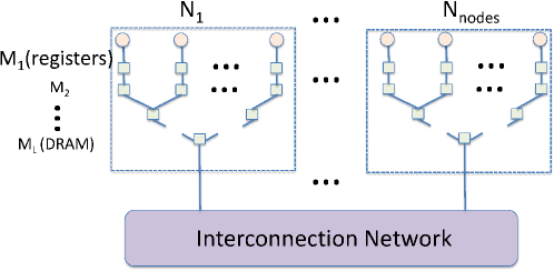
Figure 1: Distributed-memory system

Definition 6 (Parallel RBW (P-RBW) pebble game)

Let $\textit{C}=(I,V,E,O)$ be a CDAG. Given for each level $1\leq l\leq L,$ $N_{l}\times S_{l}$ number of red pebbles of different shades $R^{1}_{l},~{}R^{2}_{l},\cdots,~{}R^{N_{l}}_{l}$, respectively, and unlimited blue and white pebbles, with a blue pebble on each input vertex, a complete game is any sequence of steps using the following rules that results in a final state with white pebbles on all vertices and blue pebbles on all output vertices:

• A level-$L$ pebble, $R^{i}_{L}$ can be placed on any vertex that has a blue pebble; a white pebble is also placed along with the shade of red pebble, unless the vertex already has a white pebble on it.

• A blue pebble can be placed on any vertex that has a level-$L$ pebble on it.

• A level-$L$ pebble, $R^{i}_{L}$ can be placed on any vertex that has another level-$L$ shade pebble $R^{j}_{L}$.

• For $1\leq l<L$, a level-$l$ red pebble, $R^{i}_{l}$ can be placed on any vertex that has a level-$l+1$ pebble $R^{j}_{l+1}$ where $R^{i}_{l}$ is in a cache that is a child of the cache that holds $R^{j}_{l+1}$.

• For $1<l\leq L$, a level-$l$ red pebble, $R^{j}_{l}$ can be placed on any vertex that has a level-$l-1$ pebble $R^{i}_{l-1}$ where $R^{i}_{l-1}$ is in a cache that is a child of the cache that holds $R^{j}_{l}$.

• If a vertex $v$ does not have a white pebble and all its immediate predecessors have level-1 red pebbles on them, then a level-1 red pebble $R^{p}_{1}$ along with a white pebble may be placed on $v$; here $p$ is the index of the processor that comuptes vertex $v$.

• Any shade of red pebble may be removed from any vertex (reuse storage).

4 I/O Lower Bound for parallel machines

In this section, we provide the necessary tools to analyze the lower bounds for the parallel case. In particular, we consider two distinct cases of data movement:

1. data movement along the memory hierarchy within a processor, which we call the vertical data movement;

2. data movement across processors, which we call the horizontal data movement.

4.1 I/O Lower Bound for Vertical Data Movement

The hierarchical memory can enforce either the inclusion or exclusion policy. In case of inclusive hierarchical memory, when a copy of a value is present at a level-$l$, it is also maintained at all the levels $l+1$ and higher. These values may or may not be consistent with the values held at the lower levels. The exclusive cache, on the other hand, does not guarantee that a value present in the cache at level-$l$ will be available at the higher levels $\geq l+1$. The following result is derived for the inclusive case. But, they also hold true for the exclusive case, where the difference lies only in the number of red pebbles that we consider in the corresponding two-level pebble game.

Theorem 5 (Vertical I/O Cost)

Let $\textit{C}=(I,V,E,O)$ be a CDAG. Consider any valid P-RBW game on $C$; for this valid game, consider the level-$l$ storage $j$ with the maximum number of $R5$ transitions placing a $R^{j}_{l}$ shade red pebble. The corresponding amount of move down transitions to this shade is at least $IO_{1}(C,S_{l-1}\times N_{l-1})/N_{l}$, where $IO_{1}(C,S)$ is the I/O lower bound of $C$ for a single processor with local memory of size $S$.

Proof. Consider a P-RBW game of $C$ that minimizes the overall amount of I/O between levels $k<l$ and level $l$ storage. This amount of I/O will be bounded by $IO_{1}(C,S_{l-1}\times N_{l-1})$. Consider one of the $N_{l}$ caches with the maximum amount of I/O. It will be bounded by $IO_{1}(C,S_{l-1}\times N_{l-1})/N_{l}$. $\Box$

Theorem 6 (Vertical I/O Cost)

Let $\textit{C}=(I,V,E,O)$ be a CDAG. Consider any valid P-RBW game on $C$; for this valid game, consider the level-$l$ storage $j$ with the maximum number of $R5$ transitions placing a $R^{j}_{l}$ shade red pebble. The corresponding amount of move down transitions to this shade is at least
$\left[|V|/(U(C,2S_{l-1})\times N_{l})-N_{l-1}/N_{l}\right]\times S_{l-1}\approx\frac{|V|\times S_{l-1}}{U(C,2S_{l-1})\times N_{l}}$ where $|V|$ is the total amount of work, $U(C,2S)$ is the largest 2S-partition of the CDAG $C$.

Proof. Consider a P-RBW game of $C$ that minimizes the overall amount of I/O between levels $k<l$ and level-$l$ storage. Consider the group of $P/N_{l}$ processors that do the more computation in this game. They do at least $|V|/N_{l}$ amount of work. Let us consider the partition of those $P/N_{l}$ processors into $N_{l-1}/N_{l}$ sets of $P/N_{l-1}$ processors that share the same level-$l-1$ storage unit. Each set of processor (that we denote $P^{i}$ with $0<i\leq N_{l-1}/N_{l}$) does at least $\alpha^{i}\times\frac{|V|}{N_{l}}$ amount of work where $\sum_{i}\alpha^{i}=1$. We let $V^{i}$ be the subset of nodes of $C$ fired by $P^{i}$.

Let us denote $S_{l-1}$ by $S$ to simplify the notations. The goal is to show that each $P^{i}$ performs at least $\left[|V|^{i}/U(C,2S)-1\right]\times S$ I/O to its level-$l$ storage where $U(C,2S)$ is the largest 2S-partition (RBW pebble game) of CDAG $C$. Consider an RBW game of $C$ with $S$ red pebbles. Consider the partitioning of the game into $C_{1},\cdots,C_{h}$ used in the proof of Theorem 1 for RBW. We let $V_{j}^{i}$ be the set of vertices of $V^{i}$ fired in $C_{j}$ ($\bigcup V_{j}^{i}=V^{i}$; $V_{j}^{i}\cap V_{j}^{\prime i}=\emptyset$ for $j\neq j^{\prime}$). With the usual reasoning we can prove that $|In(V_{j}^{i})|\leq 2S$ and $|Out(V_{j}^{i})|\leq 2S$ ie each $V_{j}^{i}$ is a 2S-partition of $C$. Thus for each $j$, $|V_{j}^{i}|\leq U(C,2S)$. Now from a valid P-RBW game, we can build a valid RBW game where the restriction to $V^{i}$ matches the P-RBW game. By construction, each $V_{j}^{i}$ is associated to at least $S$ I/O to level-$l$ storage in the P-RBW game. Thus the total amount of I/O for $P^{i}$ is at least $\left[|V^{i}|/|V_{j}^{i}|-1\right]\times S\geq\left[W^{i}/U(C,2S)-1\right]\times S$.

If we sum up the I/O of each set of processors with our level-$l$ storage unit associated to the $P/N_{l}$ processors that do the more computation in the game we get $\left[W/N_{l}-N_{l-1}/N_{l}\times U(C,2S)\right]\times S/U(C,2S)=\left[W/(U(C,2S).N_{l})-N_{l-1}/N_{l}\right]\times S$ $\Box$

4.2 I/O Lower Bound for Horizontal Data Movement

The following theorem extends the S-partitioning technique to the horizontal case.

Theorem 7 (Horizontal I/O Cost)

Let $\textit{C}=(I,V,E,O)$ be a CDAG. Consider any valid P-RBW game on C; for this valid game, consider the level-$L$ storage $i$ whose group of processors $P^{i}$ perform the maximum number of $R6$ (compute) transitions. The corresponding amount of remote get transitions is atleast $\left(\frac{\left|V\right|}{U(C,2S_{L}).P_{i}}-1\right)\times S_{L}$

Proof.

We let $V^{i}$ be the subset of nodes of C fired by $P^{i}$. Let us denote $S_{L}$ by S for simplicity. Consider an RBW game of $C$ with $S$ red pebbles. Consider the partitioning of the game into $C_{1},\cdots,C_{h}$ used in the proof of Theorem 1 for RBW. We let $V_{j}^{i}$ be the set of vertices of $V^{i}$ fired in $C_{j}$ ($\bigcup V_{j}^{i}=V^{i}$; $V_{j}^{i}\cap V_{j}^{\prime i}=\emptyset$ for $j\neq j^{\prime}$). With the usual reasoning we can prove that $|In(V_{j}^{i})|\leq 2S$ and $|Out(V_{j}^{i})|\leq 2S$ ie each $V_{j}^{i}$ is a 2S-partition of $C$. Thus for each $j$, $|V_{j}^{i}|\leq U(C,2S)$. Now from a valid P-RBW game, we can build a valid RBW game where the restriction to $V^{i}$ matches the P-RBW game. By construction, each $V_{j}^{i}$ is associated to at least $S$ I/O operations in the P-RBW game. Thus the total amount of I/O for $P^{i}$ is at least $\left[|V^{i}|/|V_{j}^{i}|-1\right]\times S\geq\left[W^{i}/U(C,2S)-1\right]\times S$.

Since the group $P^{i}$ performs maximum number of computations, $W^{i}\geq W/P$. Hence, the total amount of remote get of processors $P^{i}$ is atleast $\left((\left|V\right|/(U(C,2S_{L}).P_{i}))-1\right)\times S_{L}$ $\Box$

5 Evaluation

A processor’s machine balance is the ratio of the peak memory bandwidth to the peak floating-point performance. Lower and upper bound analysis of the algorithms can help us identify whether an algorithm is bandwidth bound at different levels of memory hierarchy.

The lower bound results can be related to the architectural machine balance as below: Consider a multi-node/multi-core system with $P$ processors. Let $N_{l}$ be the total number of memory units available at level $l$. Consider a memory unit at level $l$, $M_{l}^{i}$, that incurs the maximum communication. $M_{l}^{i}$, is shared by the processor set $P_{l}^{i}$, such that $\left|P_{l}^{i}\right|=P/N_{l}$. Let $\mathcal{B}_{l}^{i}$ denote the total available memory bandwidth between $M_{l}^{i}$ and all its children at level $l-1$.

Let $\textit{C}=(I,V,E,O)$ be the CDAG of the algorithm being analyzed and $\textit{C}^{l,i}\subset C$ be the sub-CDAG executed by the processors $P_{l}^{i}$. The time taken for execution of C is given by

$$T\geq max(T_{l}^{i},T_{comp})$$

where, $T_{l}^{i}$ denotes the communication time at $M_{l}^{i}$ and $T_{comp}$ denotes the computation time for C.

For the algorithm to be not bound by memory at level $l$,

$$T_{l}^{i}\leq T_{comp}$$ (4)

Let $\textit{IO}_{l}^{i}$ denote the amount of data transferred between $M_{l}^{i}$ and all its children at level $l-1$ for the execution of a $C_{l}^{i}$. Then,

$$T_{l}^{i}=\frac{\textit{IO}_{l}^{i}}{\mathcal{B}_{l}^{i}}\geq\frac{LB_{l}^{i}}{\mathcal{B}_{l}^{i}}$$ (5)

where, $LB_{l}^{i}$ denotes the lower bound on the amount of data transfer at memory unit $M_{l}^{i}$ for any valid execution of $\textit{C}_{l}^{i}$. The computation time of C is given by ($F$ below indicates FLOPs)

$$T_{comp}\geq\frac{\left|V\right|}{P}\times\frac{1}{F}$$ (6)

From Equations (4), (5) and (6), we have,

$$\frac{LB_{l}^{i}}{\mathcal{B}_{l}^{i}}\leq\frac{\left|V\right|}{P}\times\frac{1}{F}\quad\mbox{ or }\quad\frac{LB_{l}^{i}}{\left|V\right|}\leq\frac{\mathcal{B}_{l}^{i}}{P}\times\frac{1}{F}$$

As $P=\left|P_{l}^{i}\right|\times N_{l}^{i}$,

$$\frac{LB_{l}^{i}\times N_{l}^{i}}{\left|V\right|} \leq \frac{\mathcal{B}_{l}^{i}}{\left|P_{l}^{i}\right|\times{F}}$$ (7)

The term at the right-hand side of equation 7 is the machine balance value for the machine.

Hence, any algorithm that fails to satisfy the condition 7, will be bandwidth bound at level $l$ irrespective of any optimizations we do to the code.

Through similar argument, given that $UB_{l}^{i}$ is the upper bound on the minimum amount of data transfer required by the algorithm at memory unit $M_{l}^{i}$, we can show that if the algorithm is communication bound, then it definitely satisfies the condition,

$$\frac{UB_{l}^{i}\times N_{l}^{i}}{\left|V\right|}\geq\frac{\mathcal{B}_{l}^{i}}{\left|P_{l}^{i}\right|\times{F}}$$ (8)

Hence, if an algorithm fails to satisfy condition 8, we can safely conclude that there is atleast one execution order of C that is not constrained by the memory bandwidth at level $l$.

In particular, we were interested in understanding the memory bandwidth requirements (1) between the main memory and L2 cache within each processor, and, (2) between different processors for various algorithms. For simplicity, we assume that the L2 cache is shared by all the cores within a node, which is common in practice. Our claim is that the vertical data movement between the main memory and L2 cache will be the major bottleneck in the future machines, compared to the inter-node data movement. We show that this is true for various algorithms by comparing the lower bound for vertical data movement and the upper bound for horizontal data movement against the machine balance values of different machines.

Considering the particular case of data movement between L2 cache and the main memory, equation 7 becomes,

$$\frac{LB_{vert}\times N_{nodes}}{\left|V\right|} \leq \frac{\mathcal{B}_{vert}}{N_{cores}\times{F}}$$ (9)

where, $LB_{vert}$ is the vertical data movement lower bound, $\mathcal{B}_{vert}$ is the total bandwidth between DRAM and L2 cache, $N_{nodes}$ represents the number of nodes in the system, and $N_{cores}$ represents the number of cores within each node. Similarly, considering the inter-node communication, equation 8 becomes,

$$\frac{UB_{horiz}\times N_{nodes}}{\left|V\right|}\geq\frac{\mathcal{B}_{horiz}}{N_{cores}\times{F}}$$ (10)

where, $UB_{horiz}$ and $\mathcal{B}_{horiz}$ represent the upper bound on the horizontal data movement cost and inter-processor communication bandwidth, respectively.

Specifications for some of the powerful computing systems are shown in table 1. We plan to use this list to compare various algorithms in the following sections to determine their memory requirement constraints.

Table 1: Specifications of various computing systems

Machine	$\mathbf{N_{nodes}}$	Mem. (GB)	L2/L3 cache (MB)	Vertical balance (words/FLOP)	Horiz. balance (words/FLOP)
IBM BG/Q	2048	16	32	0.052	0.049
Cray XT5	9408	16	6	0.0256	0.058

Before we present the results for various numerical algorithms, we provide a brief introduction to the type of problem solved by these numerical solvers, in the following section.

5.1 Brief introduction on discretization

Many real world problems involve solving partial differential equations (PDEs). As an example, consider the heat flow on a long thin bar of unit length, of uniform material and insulated, so that the heat can enter and exit only at the boundaries (refer Fig. 2(a)). Let $u(x,t)$ represent the temperature at position $0\leq x\leq 1$, and time $t\geq 0$. The objective is to determine the change in temperature over time ($u(x,t)$). The governing heat equation that describes this distribution of heat is given by the PDE:

$$\frac{du(x,t)}{dt}=\alpha\times\frac{d^{2}u(x,t)}{dx^{2}}$$

where, $\alpha$ is the thermal diffusivity of the bar. (For mathematical treatment, it is sufficient to consider $\alpha=1$).

Figure 2: One-dimensional heat flow problem

Since the problem is continuous, to numerically solve the heat equation, it needs to be discretized (through finite difference approximation) to reduce it to a finite problem. In the discretized problem, the values of $u(x,t)$ are only computed at discrete points at regular intervals of the bar, called the computational grid or mesh. The state variables at these grid points are given by $u(x(i),t(m))$, where $x(i)=i\times h,~{}0\leq i\leq n+1=1/h$ and $t(m)=m\times k$; $h$ and $k$ are the grid spacing and timestep, respectively. Fig. 2(b) shows an example grid obtained by discretizing the one-dimensional bar.

The governing equation, after discretization, yields the following equation at grid point $i$ and timestamp $m+1$.

$$\frac{-a}{2}\times U(i-1,m+1)+(1+a)\times U(i,m+1)-\frac{a}{2}\times U(i+1,m+1)=$$

$$\frac{a}{2}\times U(i-1,m)+(1-a)\times U(i,m)+\frac{a}{2}\times U(i+1,m)$$

where, $U(p,q)=u(x(p),t(q))$ and $a=k/h^{2}$. Hence, the solution to the problem involves solving a linear system of $n-1$ equations at each timestamp till convergence. Each timestamp $m+1$ is dependant on values of the previous timestamp $m$.

This linear system can be represented in tridiagonal matrix form as follows:

$$\left(\begin{smallmatrix}1+a&-\frac{a}{2}&&&&&\\ -\frac{a}{2}&1+a&-\frac{a}{2}&&&&\\ &-\frac{a}{2}&1+a&-\frac{a}{2}&&&\\ &&\ddots&\ddots&\ddots&&&\\ &&&-\frac{a}{2}&1+a&-\frac{a}{2}&\\ &&&&-\frac{a}{2}&1+a\\ \end{smallmatrix}\right)\times\left(\begin{smallmatrix}U(1,m+1)\\ U(2,m+1)\\ U(3,m+1)\\ \vdots\\ U(n-1,m+1)\\ U(n,m+1)\\ \end{smallmatrix}\right)=\left(\begin{smallmatrix}b(1,m)\\ b(2,m)\\ b(3,m)\\ \vdots\\ b(n-1,m)\\ b(n,m)\end{smallmatrix}\right)$$ (11)

where, $b(i,m)$ represents the right-hand side of the $i$-th equation at timestamp $m+1$. Solving this linear system of the form $Ax=b$ for vector $x$ provides the solution to the original problem. In general, for a $d$-dimensional problem, the coefficient matrix is of size $n^{d}$-by-$n^{d}$, while the vectors are of size $n^{d}$. In practice, the elements of the matrix are not explicitly stored. Instead, their values are directly embedded in the program as constants thus eliminating the space requirement and the associated I/O cost for the matrix.

In practice, the prohibitive problem size prevents direct solution of (11). Hence, various iterative methods were developed to efficiently solve such large linear systems. The following section derives the vertical and horizontal data movement bounds for some of these iterative linear system solvers using the results from Sections 3 and 4 and compares it against the machine balance values.

5.2 Conjugate Gradient (CG)

The Conjugate Gradient method [15] is suitable for solving symmetric positive-definite linear systems. CG maintains 3 vectors at each timestep - the approximate solution $x$, its residual $r=Ax-b$, and a search direction $p$. At each step, $x$ is improved by searching for a better solution in the direction $p$.

Each iteration of CG involves one sparse matrix-vector product, three vector updates, and three vector dot-products. The complete pseudocode is shown in Fig. 3.

⬇

1function CG

2 $x$ is the initial guess

3 $r\leftarrow b-Ax$

4 $p\leftarrow r$

5 do

6 $v\leftarrow Ap$ //SpMV

7 $a\leftarrow\left\langle\langle r,r\right\rangle\rangle/\left\langle\langle p,v\right\rangle\rangle$ //Dot-products

8 $x\leftarrow x+ap$ //saxpy

9 $r_{new}\leftarrow r-av$ //saxpy

10 $g\leftarrow\left\langle\langle r_{new},r_{new}\right\rangle\rangle/\left\langle\langle r,r\right\rangle\rangle$ //Dot-products

11 $p\leftarrow r_{new}+gp$ //saxpy

12 $r\leftarrow r_{new}$

13 until $\left(\left\langle\langle r_{new},r_{new}\right\rangle\rangle~{}is~{}small~{}enough\right)$

14end function

Figure 3: Conjugate Gradient method

5.2.1 Vertical data movement cost

We provide the lower bound for the amount of data movement between different levels of hierarchy.

Theorem 8 (Min-cut based I/O lower bound for CG)

For a $d$-dimensional grid of size $n^{d}$, the minimum I/O cost to solve the linear system using CG, $Q$, satisfies $Q\geq 6n^{d}T/P$, when $n\gg\textit{S}$; where, $T$ represents the number of outer loop iterations.

Proof. Consider the vertex $\upsilon_{x}$, corresponding to the scalar $a$ at line 7. The $2n^{d}$ predecessor vertices of $\upsilon_{x}$, corresponding to vectors $p$ and $v$, have disjoint paths to the $\textsf{Desc}(\upsilon_{x})$ (due to computations in lines 8 and 9, respectively). This gives us a wavefront of size $\left|W_{G}^{min}(\upsilon_{x})\right|=2n^{d}$. Similarly, considering the vertex, $\upsilon_{y}$, corresponding to the scalar $g$, at line 10, we obtain a wavefront of size $\left|W_{G}^{min}(\upsilon_{y})\right|=n^{d}$, due to the disjoint paths from the predecessors $r_{new}$ to $\textsf{Desc}(x)$ (due to the computation at line 11).

Recursively applying theorem 4 on the complete CDAG, C, provides us $T$ sub-CDAGs, $\textit{C}_{1},~{}\textit{C}_{2},\dots,\textit{C}_{T}$, corresponding to each outer loop iteration. (Vertices of vector $p$ due to line 11 are shared between neighboring sub-CDAGs). Further, non-disjointly sub-dividing each of these sub-CDAGs, $\textit{C}_{i}$, into $\textit{C}_{i_{|x}}and\textit{C}_{i_{|y}}$ (vertices of vector $r_{new}$ from line 9 are shared between $\textit{C}_{i_{|x}}and\textit{C}_{i_{|y}}$), to decompose the effects of wavefronts $W_{G}^{min}(\upsilon_{x})$ and $W_{G}^{min}(\upsilon_{y})$, we obtain a lower bound of,

Q $$\geq T\times(2(2n^{d}-S))+T\times(2(n^{d}-S))$$

$$= T\times(2(3n^{d}-2S))$$

which tends to $6n^{d}T$ as $n$ becomes $\gg S$. Finally, application of theorem 5 provides a lower bound of $6n^{d}T/P$ for the parallel case. $\Box$

5.2.2 Horizontal data movement cost

Let us assume that the input grid is block partitioned among the processors. Hence, each processor holds the input data corresponding to its local grid points and computes the data needed by those grid points. Let $B=n/N_{nodes}^{1/d}$ be the size of the block along each dimension. Computating the sparse matrix-vector product, at line 6 in Fig. 3, majorly contributes to the communication cost. This involves getting the values of the ghost cells from the neighboring processors. This value is given by $(B+2)^{d}-B^{d}$. If Q is the minimum I/O cost for executing CG, then,

Q $$\leq ((B+2)^{d}-B^{d})\times T$$

$$= (B^{d}+{d\choose 1}B^{d-1}2^{1}+{d\choose 2}B^{d-2}2^{2}$$

$$+\cdots+{d\choose d-1}B^{1}2^{d-1}+{d\choose d}B^{0}2^{d}B^{d})\times T$$

$$= O(2dB^{d-1}T)$$

5.2.3 Analysis

Equations 9 and 10 provided us conditions to determine the vertical and horizontal memory constraints of the algorithms. We will use them to show that the running time of CG is mainly constrained by the vertical data movement.

Consider a 3D-grid ($d=3$), with $n=1000$. The total operation count (FLOP) is $20n^{3}T$. The I/O lower bound per node is given by $\displaystyle\frac{6n^{3}T}{P}\times N_{cores}=\frac{6n^{3}T}{N_{nodes}}$. Hence,

$$\frac{LB_{vert}\times N_{nodes}}{\left|V\right|}=\frac{\left(6n^{3}T/N_{nodes}\right)\times N_{nodes}}{20n^{3}T}=\frac{6}{20}=0.3$$

This value is higher than the machine balance value of any machine (refer table 1), leaving condition 9 unsatisfied. This shows that CG will be unavoidably bandwidth bound along the vertical direction for the problems that cannot fit into the cache. The only way to improve the performance would be to increase the main memory bandwidth.

On the other hand, let us consider the horizontal data movement cost.

$$\frac{UB_{horiz}\times N_{nodes}}{\left|V\right|}=\frac{6B^{2}T\times N_{nodes}}{20n^{3}T}$$

$$= \frac{6\left(n/N_{nodes}^{(1/3)}\right)^{2}N_{nodes}}{20n^{3}}=\frac{6N_{nodes}^{(1/3)}}{20n}$$

This value easily falls below the machine balance values of various machines, indicating that the inter-node communication is not a bottleneck for the execution of CG algorithm.

5.3 Generalized Minimal Residual (GMRES)

The Generalized Minimum Residual (GMRES) [22] method is designed to solve non-symmetric linear systems. The most popular form of GMRES is based on the modified Gram-Schmidt procedure. The method arrives at the solution after $m$ iterations, where $m$ represents the dimension of a linear subspace–called Krylov subspace–formed by an orthogonal basis. At each step, $x$ is improved by searching for a better solution along the direction of one of these basis vectors.

Each outer loop iteration $i$ of GMRES involves one sparse matrix-vector product, $(i+1)$ vector dot-products and $i$ vector updates. The complete pseudocode is shown in Fig. 4.

⬇

1function GMRES

2 $x_{0}$ is the initial guess

3 $r_{0}\leftarrow b-Ax_{0}$

4 $v_{0}\leftarrow r_{0}/\left\lVert r_{0}\right\rVert_{2}$

5 do

6 $w\leftarrow Av_{i}$ //SpMV

7 for $j=0,1,\dots,i$ do

8 $h_{j,i}\leftarrow\left\langle\langle w,v_{j}\right\rangle\rangle$ //Dot-product

9 end do

10 $v^{\prime}_{i+1}\leftarrow w-\sum_{j=1}^{i}h_{j,i}v_{j}$ //saxpy’s

11 $h_{i+1,i}\leftarrow\left\lVert v^{\prime}_{i+1}\right\rVert_{2}$ //Dot-product

12 $v_{i+1}\leftarrow v^{\prime}_{i+1}/h_{i+1,i}$

13 Apply Givens rotations to $h_{:,i}$

14 until (convergence)

15 $y\leftarrow\operatorname*{arg\,min}{\left\lVert Hy-\left\lVert r_{0}\right\rVert_{2}e_{1}\right\rVert_{2}}$

16 $x\leftarrow x_{0}+Vy$

17end function

Figure 4: Basic GMRES

5.3.1 Vertical data movement cost

Theorem 9 (Min-cut lower bound for GMRES)

For a $d$-dimensional grid of size $n^{d}$, the minimum I/O cost to solve the linear system using GMRES, $Q$, satisfies $Q\geq 6n^{d}m/P$, when $n\gg\textit{S}$; where, $m$ represents the number of outer loop interations.

Proof. Consider the vertex $\upsilon_{x}$ corresponding to the result of the inner product at iteration $j=i$ at line 8. This is a reduction operation with the predecessors of $\upsilon_{x}$ being the vertices of vectors $w$ and $v_{i}$ of size $n^{d}$. All of these $2n^{d}$ predecessor vertices (of vectors $w$ and $v_{i}$) have a disjoint path to the successor of vertex $\upsilon_{x}$ due to the computation at line 10, leading to a wavefront of size $\left|W_{G}^{min}(\upsilon_{x})\right|=2n^{d}$. By similar argument, by taking vertex $\upsilon_{y}$ as the result of the computation at line 11, we obtain wavefront of size $\left|W_{G}^{min}(\upsilon_{y})\right|=n^{d}$ due to the vertices of vector $v^{\prime}_{i+1}$.

Application of theorem 4 recursively allows us to non-disjointly decompose the vertices of each iteration of loop-$i$ into $m$ sub-DAGs, $\textit{C}_{1},~{}\textit{C}_{2},\dots,\textit{C}_{m}$, with vertices of vector $v_{i+1}$ (computed at line 12) being shared by sub-DAGs $\textit{C}_{i}$ and $\textit{C}_{i+1}$. Each of these sub-DAGs, $\textit{C}_{i}$ can be further non-disjointly partitioned into $\textit{C}_{i_{|x}}and\textit{C}_{i_{|y}}$, to decompose the effects of wavefronts $W_{G}^{min}(\upsilon_{x})$ and $W_{G}^{min}(\upsilon_{y})$ into separate sub-DAGs (with vertices of $v^{\prime}_{i+1}$ from line 10 being shared between sub-CDAGs $\textit{C}_{i_{|x}}and\textit{C}_{i_{|y}}$). This gives us $m$ sub-DAGs, each with wavefront of size $2n^{d}$, and $m$ sub-DAGs with wavefront of size $n^{d}$.

Applying Lemma 2 on these sub-DAGs gives us a lower bound of,

Q $$\geq m\times(2(2n^{d}-S))+m\times(2(n^{d}-S))$$

$$= m\times(2(3n^{d}-S))$$

which tends to $6n^{d}m$ as $n$ grows. Finally, application of theorem 5 provides a lower bound of $6n^{d}m/P$ for the parallel case. $\Box$

5.3.2 Horizontal data movement cost

The horizontal data movement trend for GMRES is similar to CG (Sec. 5.2.2). Hence, upon applying similar analysis on the GMRES algorithm, we obtain an upper bound of

$$\textit{Q}=O(2dB^{d-1}m)$$

where, $B$ is the block size along each dimension.

5.3.3 Analysis

Consider a 3D-grid ($d=3$), with $n=1000$. The total number of operations for GMRES is $20n^{3}m+n^{3}m^{2}$. The vertical data movement cost per FLOP,

$$\frac{LB_{vert}\times N_{nodes}}{\left|V\right|} = \frac{6}{m+20}$$

For smaller values of $m$, this value stays higher than the machine balance value for current systems. But as $m$ gets higher, the computational time begins to dominate the vertical data movement cost.

The Horizontal data movement cost per FLOP is given by,

$$\frac{UB_{horiz}\times N_{nodes}}{\left|V\right|} = \frac{6N_{nodes}^{(1/3)}}{nm}$$

This value is orders of magnitude smaller than the machine balance values of current systems, showing that the algorithm is not inter-node bandwidth bound.

On the other hand, for the vertical data movement, as the lower and upper bounds do not match, it is not possible to draw a decisive conclusion unless the rate of convergence value, $m$ is known for the problem.

5.4 Jacobi Method

Jacobi’s method involves stencil computations, that begins with an initial guess for the unknown vector $x$ and iteratively replaces the current approximate solution at each grid point by a weighted average of its nearest neighbors on the grid. Hence, the information at one grid point can only propogate to its adjacent grid points in one iteration. Thus, it takes atleast $n$ steps to propogate the information throughout the grid and reach to the solution.

5.4.1 Vertical data movement cost

In this section, we derive the I/O lower bound for Jacobi computation on a $d$-dimensional grid. We provide the proof for a 2D-grid below, which can be generalized to a grid of $d$-dimensions as shown later.

Theorem 10 (I/O lower bound for Jacobi)

For the $9$-points Jacobi of size $n\times n$ with $T-1$ time steps, the minimum I/O cost, Q, satisfies $\textit{Q}\geq\frac{N^{2}T}{4P\sqrt{2\textit{S}}}$.

Proof. The CDAG of Jacobi computation has the property that all inputs can reach all outputs through vertex-disjoint paths. These vertex-disjoint paths will be called lines, for simplicity. Let $F(d)$ denote a monotonically increasing function such that for any two vertices $u$ and $v$ on the same line that are atleast $d$ apart, $F(d)$ has the following properties: (1) none of these $F(d)$ vertices belong to the same line; (2) Each of these vertices belongs to a path connecting $u$ and $v$. In [16, Theorem 5.1], Hong & Kung show that the serial I/O lower bound, $Q_{s}$, for the CDAG with the above mentioned properties can be bounded by $Q_{s}\geq L/(2.(F^{-1}(2\textit{S})+1))$, where $L$ is the total number of vertices on the lines. From the structure of the CDAG for 2D-Jacobi computation, it can be seen that $F^{-1}(2S)=2\sqrt{2\textit{S}}-1$. Hence, we have, $Q_{s}\geq n^{2}T/4\sqrt{2\textit{S}}$. Finally, from Theorem 5, we have the parallel I/O cost, $Q\geq n^{2}T/4P\sqrt{2\textit{S}}$. $\Box$

With the similar reasoning, the I/O lower bound can be extended to higher dimensions, leading to the I/O cost of $Q\geq n^{d}T/4.P.(2\textit{S})^{1/d}$, for a $d$-dimensional grid.

It could be seen that this lower bound is tight as the tiled stencil computation algorithm has the I/O cost that matches this bound.

5.4.2 Horizontal data movement cost

The horizontal data movement cost is due to the communication of the ghost cells. This amounts to the I/O cost of $4BT$, where $B$ is the block size along each dimension.

5.4.3 Analysis

From (7) and Theorem 6, and since the lower bound derived in Theorem 10 is tight, for the computation to be not bandwidth-bound along the vertical direction, the following relation has to be satisfied:

$$\frac{\mathcal{B}^{i}_{l}}{\left|P^{i}_{l}\right|\times{F}} \geq \frac{LB^{i}_{l}\times N^{i}_{l}}{\left|V\right|}$$

$$= \frac{(\left|V\right|.\textit{S}_{l-1}/U(C,2S_{l-1}).N_{l}^{i})\times N_{l}^{i}}{\left|V\right|}$$

$$= \frac{\textit{S}_{l-1}}{U(C,2S_{l-1})}$$

From Theorem 10, for a $d$-dimensional Jacobi, $U(C,2S_{l-1})=4S_{l-1}(2S_{l-1})^{1/d}$. Hence,

$$\frac{\mathcal{B}^{i}_{l}}{\left|P^{i}_{l}\right|\times{F}}\geq\frac{1}{4(2S_{l-1})^{1/d}}$$

From Table 1, for IBM BG/Q, the vertical machine balance parameter for the data movement between main memory and L2 cache is 0.052. Hence, ${1}/{4(2S_{2})^{1/d}}\leq 0.052$ or, $d\leq 0.21\log(2\textit{S}_{2})$. Substituting the value of $S_{2}=4$ MWords, we get, $d\leq 4.83$.

By following similar reasoning and considering the machine parameters for the data movement between L2 and L1 caches, for the computation to be not bandwidth-bound, $d\leq 96$.

This shows that the data movement between main memory and L2 cache is critical for the preformance and the algorithm is bandwidth bound only for higher dimensional stencils of dimension $d\geq 5$, which are not common in practice.

6 Related Work

Hong & Kung provided the first characterization of the I/O complexity problem using the red/blue pebble game and the equivalence to 2S-partitioning of CDAGs [16]. Their 2S-partitioning approach uses dominators of incoming edges to partitions but does not account for the internal structure of partitions. In this paper, in addition to using the 2s-partitioning technique, we also use an alternate lower bound approach that models the internal structure of CDAGs, and uses graph mincut as the basis. In addition, Hong & Kung’s original model does not lend itself easily to development of effective lower bounds for a CDAG from bounds for component sub-graphs. With a change of the pebble game model to the RBW game, we were able to use CDAG decomposition to develop tight composite lower bounds for inhomogeneous CDAGs.

Several works followed Hong & Kung’s work on I/O complexity in deriving lower bounds on data accesses [2, 1, 18, 6, 5, 23, 24, 19, 20, 29, 13, 3, 4, 8, 28, 26]. Aggarwal et al. provided several lower bounds for sorting algorithms [2]. Savage [23, 24] developed the notion of $S$-span to derive Hong-Kung style lower bounds and that model has been used in several works [19, 20, 26]. Irony et al. [18] provided a new proof of the Hong-Kung result on I/O complexity of matrix multiplication and developed lower bounds on communication for sequential and parallel matrix multiplication. More recently, Demmel et al. have developed lower bounds as well as optimal algorithms for several linear algebra computations including QR and LU decomposition and all-pairs shortest paths problem [3, 4, 13, 28]. Bilardi et al. [6, 5] develop the notion of access complexity and relate it to space complexity. Bilardi and Preparata [7] developed the notion of the closed-dichotomy size of a DAG $G$ that is used to provide a lower bound on the data access complexity in those cases where recomputation is not allowed. Our notion of schedule wavefronts is similar to the closed-dichotomy size in their work; but, unlike the work of [7], we use it do develop an effective automated heuristic to compute lower bounds for CDAGs. Extending the scope of the Hong & Kung model to more complex memory hierarchies has been the subject of some research. Savage provided an extension together with results for some classes of computations that were considered by Hong & Kung, providing optimal lower bounds for I/O with memory hierarchies [23]. Valiant proposed a hierarchical computational model [29] that offers the possibility to reason in an arbitrarily complex parameterized memory hierarchy model.

Unlike Hong & Kung’s original model, several models have been proposed that do not allow recomputation of values (also referred to as “no repebbling”) [3, 4, 5, 27, 19, 23, 24, 26, 9, 18, 20, 21]. Savage [23] develops results for FFT using no repebbling. Bilardi and Peserico [5] explore the possibility of coding a given algorithm so that it is efficiently portable across machines with different hierarchical memory systems, without the use of recomputation. Ballard et al. [3, 4] assume no recomputation is allowed in deriving lower bounds for linear algebra computations. Ranjan et al. [19] develop better bounds than Hong & Kung for FFT using a specialized technique adapted for FFT-style computations on memory hierarchies. Ranjan et al. [20] derive lower bounds for pebbling r-pyramids under the assumption that there is no recomputation. Recently, Ranjan et al. [21] develop a technique for binomial graphs. Very recent work from U.C. Berkeley [8] has developed a very novel approach to developing parametric I/O lower bounds applicable/effective for a class of nested loop computations but is either inapplicable or produces weak lower bounds for other computations (e.g., stencil computations, FFT, etc.).

The P-RBW game developed in this paper extends the parallel model for shared-memory architectures by Savage and Zubair [25] to also include the distributed-memory parallelism present in all scalable parallel architectures. The works of Irony et al. [18] and Ballard et al. [3] model communication across nodes of a distributed-memory system. Bilardi and Preperata [7] develop lower bound results for communication in a distributed-memory model specialized for multi-dimensional mesh topologies. Our model in this paper differs from the above efforts in defining a new integrated pebble game to model both horizontal communication across nodes in a parallel machine, as well as vertical data movement through a multi-level shared cache hierarchy within a multi-core node.

Czechowski et al. [11, 12] consider the relationship between the ratio of an algorithm’s data movement cost to arithmetic work and the machine balance ratio of memory bandwidth to peak performance. Our analysis of algorithms in this paper involves a very similar theme as theirs and is inspired by their work, but we develop new lower bounds analysis to perform the analysis. Further, we compare and contrast data movement demands for horizontal across-node communication versus vertical within-node data movement and observe that the latter is often the more constraining factor.

7 Conclusion

Characterizing the parallel data movement complexity of a program is a cornerstone problem, that is particularly important with current and emerging power-constrained architectures where the data transfer cost will be the dominant energy and performance bottleneck. In this paper we presented an extension to the Hong and Kung red-blue pebble game model to enable development of lower bounds on data movement for parallel execution of CDAGs. The model distinguishes horizontal data movement between nodes of a distributed-memory parallel system from vertical data movement within the multi-level memory/cache hierarchy within a multi-core node. The utility of the model and the developed lower bounding techniques was demonstrated by analysis of several numerical algorithms and the garnering of interesting insights on the relative significance of horizontal versus vertical data movement for different algorithms.

References

- [1] A. Aggarwal, B. Alpern, A. K. Chandra, and M. Snir. A model for hierarchical memory. In 19th STOC, pages 305–314, 1987.
- [2] A. Aggarwal and J. S. Vitter. The input/output complexity of sorting and related problems. Commun. ACM, 31:1116–1127, 1988.
- [3] G. Ballard, J. Demmel, O. Holtz, and O. Schwartz. Minimizing communication in numerical linear algebra. SIAM J. Matrix Analysis Applications, 32(3):866–901, 2011.
- [4] G. Ballard, J. Demmel, O. Holtz, and O. Schwartz. Graph expansion and communication costs of fast matrix multiplication. J. ACM, 59(6):32, 2012.
- [5] G. Bilardi and E. Peserico. A characterization of temporal locality and its portability across memory hierarchies. Automata, Languages and Programming, pages 128–139, 2001.
- [6] G. Bilardi, A. Pietracaprina, and P. D’Alberto. On the space and access complexity of computation dags. In Graph-Theoretic Concepts in Computer Science, volume 1928 of LNCS, pages 81–92. 2000.
- [7] G. Bilardi and F. P. Preparata. Processor - Time Tradeoffs under Bounded-Speed Message Propagation: Part II, Lower Bounds. Theory Comput. Syst., 32(5):531–559, 1999.
- [8] M. Christ, J. Demmel, N. Knight, T. Scanlon, and K. Yelick. Communication Lower Bounds and Optimal Algorithms for Programs That Reference Arrays — Part 1. EECS Technical Report EECS–2013-61, UC Berkeley, May 2013.
- [9] S. A. Cook. An observation on time-storage trade off. J. Comput. Syst. Sci., 9(3):308–316, 1974.
- [10] Cray XE6. http://www.cray.com/Products/Computing/XE.aspx.
- [11] K. Czechowski, C. Battaglino, C. McClanahan, A. Chandramowlishwaran, and R. Vuduc. Balance principles for algorithm-architecture co-design. In Proceedings of the 3rd USENIX Conference on Hot Topic in Parallelism, HotPar’11, pages 9–9, 2011.
- [12] K. Czechowski and R. Vuduc. A theoretical framework for algorithm-architecture co-design. In Proceedings of the 2013 IEEE 27th International Symposium on Parallel and Distributed Processing, IPDPS ’13, pages 791–802, 2013.
- [13] J. Demmel, L. Grigori, M. Hoemmen, and J. Langou. Communication-optimal parallel and sequential QR and LU factorizations. SIAM J. Scientific Computing, 34(1), 2012.
- [14] V. Elango, F. Rastello, L.-N. Pouchet, J. Ramanujam, and P. Sadayappan. Data access complexity: The red/blue pebble game revisited. Technical Report OSU-CISRC-7/13-TR16, Ohio State University, September 2013.
- [15] M. R. Hestenes and E. Stiefel. Methods of conjugate gradients for solving linear systems, 1952.
- [16] J.-W. Hong and H. T. Kung. I/O complexity: The red-blue pebble game. In Proc. of the 13th annual ACM sympo. on Theory of computing (STOC’81), pages 326–333. ACM, 1981.
- [17] IBM Blue Gene team. The ibm blue gene project. IBM Journal of Research and Development, 57(1/2):0:1–0:6, 2013.
- [18] D. Irony, S. Toledo, and A. Tiskin. Communication lower bounds for distributed-memory matrix multiplication. J. Parallel Distrib. Comput., 64(9):1017–1026, 2004.
- [19] D. Ranjan, J. Savage, and M. Zubair. Strong I/O lower bounds for binomial and FFT computation graphs. In Computing and Combinatorics, volume 6842 of LNCS, pages 134–145. Springer, 2011.
- [20] D. Ranjan, J. E. Savage, and M. Zubair. Upper and lower I/O bounds for pebbling r-pyramids. J. Discrete Algorithms, 14:2–12, 2012.
- [21] D. Ranjan and M. Zubair. Vertex isoperimetric parameter of a computation graph. Int. J. Found. Comput. Sci., 23(4):941–, 2012.
- [22] Y. Saad and M. H. Schultz. Gmres: A generalized minimal residual algorithm for solving nonsymmetric linear systems. SIAM Journal on scientific and statistical computing, 7(3):856–869, 1986.
- [23] J. Savage. Extending the Hong-Kung model to memory hierarchies. In Computing and Combinatorics, volume 959 of LNCS, pages 270–281. 1995.
- [24] J. E. Savage. Models of computation - exploring the power of computing. Addison-Wesley, 1998.
- [25] J. E. Savage and M. Zubair. A unified model for multicore architectures. In Proceedings of the 1st international forum on Next-generation multicore/manycore technologies, page 9. ACM, 2008.
- [26] J. E. Savage and M. Zubair. Cache-optimal algorithms for option pricing. ACM Trans. Math. Softw., 37(1), 2010.
- [27] M. Scquizzato and F. Silvestri. Communication lower bounds for distributed-memory computations. CoRR, abs/1307.1805, 2013.
- [28] E. Solomonik, A. Buluç, and J. Demmel. Minimizing communication in all-pairs shortest paths. In IPDPS, 2013.
- [29] L. G. Valiant. A bridging model for multi-core computing. J. Comput. Syst. Sci., 77:154–166, Jan. 2011.