Cooperative pulses in robust quantum control: Application to broadband Ramsey-type pulse sequence elements

Abstract

A general approach is introduced for the efficient simultaneous optimization of pulses that compensate each other’ s imperfections within the same scan. This is applied to broadband Ramsey-type experiments, resulting in pulses with significantly shorter duration compared to individually optimized broadband pulses. The advantage of the cooperative pulse approach is demonstrated experimentally for the case of two-dimensional nuclear Overhauser enhancement spectroscopy. In addition to the general approach, a symmetry-adapted analysis of the optimization of Ramsey sequences is presented. Furthermore, the numerical results led to the disovery of a powerful class of pulses with a special symmetry property, which results in excellent performance in Ramsey-type experiments. A significantly different scaling of pulse sequence performance as a function of pulse duration is found for characteristic pulse families, which is explained in terms of the different numbers of available degrees of freedom in the offset dependence of the associated Euler angles.

Contents

toc

1 Introduction

Sequences of coherent and well-defined pulses play an important role in the measurement and control of quantum systems. Applications of control pulses include nuclear magnetic resonance (NMR) and electron spin resonance (ESR) spectroscopy [1, 2], magnetic resonance imaging (MRI) [3], metrology [4], quantum information processing [5] and atomic, molecular and optical (AMO) physics in general [7, 8]. Typically, pulse sequences are defined in terms of ideal pulses with unlimited amplitude and negligible duration (hard pulse limit). In practice, ideal pulses can often be approximated by rectangular pulses of finite duration, during which the phase is constant and the amplitude is set to the maximum available value.

However, simple rectangular pulses are only able to excite spins with relatively small detunings (offset frequencies) that are in the order of the maximum pulse amplitude (expressed in terms of the Rabi frequency of the pulse). For broadband applications, e.g. in NMR, ESR or optical spectroscopy with a large range of offset frequencies or highly inhomogeneous line widths, the performance of simple rectangular pulses is not satisfactory and improved performance can be achieved by using shaped or composite pulses. In addition to offset effects, experimental imperfections such as uncertainties in the flip angle and amplitude and phase transients have to be taken into account. Composite and shaped pulses can provide significantly improved performance by compensating their own imperfections [9, 10, 11, 12]. However, the improved performance of composite pulses comes at a cost: the pulses can be significantly longer compared to simple rectangular pulses with a concomitant increase in relaxation losses during the pulses if relaxation times are comparable to the pulse duration.

Optimal control theory provides efficient numerical algorithms for the optimization of time-optimal pulses [13] or of relaxation-optimized pulses [14]. With optimal control algorithms such as the gradient ascent pulse engineering (GRAPE) algorithm [15, 16, 17, 18], tens of thousands of pulse sequence parameters can be efficiently optimized. This makes it possible to design pulses without any bias towards a specific family of pulses and to explore the physical performance limits as a function of pulse duration [13, 19, 20]. This approach has provided pulses with unprecedented bandwidth and robustness with respect to experimental imperfections.

Most experiments do not only consist of a single pulse, but of highly orchestrated sequences of pulses that are separated by delays, which are either constant or which are varied in a systematic way [1]. This opens up additional opportunities to improve the overall performance of experiments beyond what is achievable by simply combining the best possible individually optimized (composite or shaped) pulses. This makes it possible to leverage on the interplay within a pulse sequence and to exploit the potential of the pulses to compensate each other’s imperfections in a given pulse sequence. The cooperativity of such pulses provides important additional degrees of freedom in the pulse sequence optimization because the individual pulses do not need to be perfect. The analysis and systematic optimization of cooperative effects between different pulses promises a better overall performance of pulse sequences and shorter pulse durations.

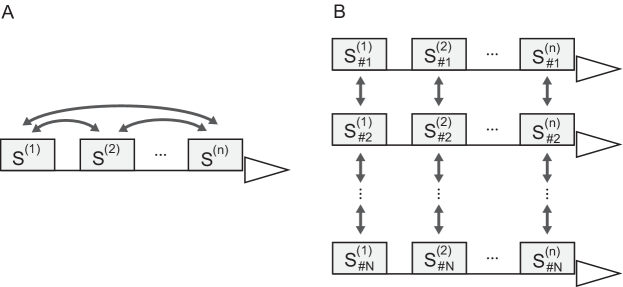
Figure 1: Two main classes of cooperative pulses are illustrated schematically: (A) same-scan cooperative pulses (s²-COOP pulses) and (B) multi-scan cooperative pulses (ms-COOP pulses). The rectangles represent (composite or shaped) pulses and the triangles indicate periods of signal acquisition. The arrows indicate cooperativity between different pulses $S^{(k)}$ and $S^{(l)}$ of the same scan (A) or between corresponding pulses $S_{\#i}^{(k)}$ and $S_{\#j}^{(k)}$ of different scans $\#i$ and $\#j$ in a multi-scan experiment [28] (B).

Here we focus on the analysis and optimization of pulse sequences consisting of individual (composite or shaped) pulses separated by delays. Together with a final detection period, such a pulse sequence is called a scan. Typically, experiments consist of a plurality of scans [1]. In the most simple form of such multi-scan experiments, a given pulse sequence is simply repeated $N$ times without any modification to accumulate the signal and hence to increase the signal-to-noise ratio. However, the power of modern coherent spectroscopy results to a large extent from the systematic variation of the pulses and delays in the different scans, enabling e.g. the suppression of artifacts by phase cycling, the selection of desired coherence transfer pathways, and multi-dimensional spectroscopy or imaging [1].

In the analysis of cooperativity between pulses, it is useful to distinguish two main classes: cooperativity between pulses in the same scan, i.e. between pulses that form a pulse sequence (cf. Fig. 1 A) and cooperativity between corresponding pulses in different scans (cf. Fig. 1 B). In order to clearly distinguish these two pulse classes, we propose the terms same-scan cooperative pulses (s²-COOP) for the first class and multi-scan cooperative pulses (ms-COOP) for the second class.

The mutual cancellation of pulse phase imperfections in the same scan has been denoted as global pulse sequence compensation [10, 21, 11]. In this approach, a series of ideal hard pulses is replaced by a series of so-called variable rotation pulses, for which the overall rotation has the same Euler angle $\beta$ but different Euler angles $\gamma$ and $\alpha$ compared to the Euler angle decomposition of the corresponding ideal hard pulses. For a special class of so-called composite LR pulses [11], an explicit procedure was derived to construct a sequence of variable angle rotation pulses that can replace ideal pulses in any given pulse sequence. In addition to constant terms, for LR pulses the $\gamma$ and $\alpha$ angles have a linear offset dependence of opposite sign, which makes it possible to balance the phase shift created by one pulse by an equal and opposite phase shift associated with the following pulse. Further examples of mutual compensation of offset-dependent phase errors are carefully chosen combinations of chirped pulses [22, 23, 24], which have also been applied to Ramsey-type sequences [25, 26]. Results of the simultaneous optimization of excitation and reconversion pulses of a double quantum filter in solid state NMR have been presented in [27], but a general approach to s²-COOP pulses has not been analyzed or discussed.

The optimization of cooperativity between corresponding pulses in different scans has been formulated as an optimal control problem [28]. An efficient algorithm was developed that makes it possible to concurrently optimize a set of ms-COOP pulses. This algorithm optimizes the overall performance of a number of scans, leading to an average signal with desired properties, where undesired terms that may be present in the signal of the individual scans cancel each other. The class of ms-COOP pulses generalizes the well-known and widely used concepts of phase-cycles [29, 30, 31] and difference spectroscopy. The power of this generalization was demonstrated both theoretically and experimentally for a variety of applications.

In this paper, a general filter-based optimal control algorithm for the simultaneous optimization of s²-COOP pulse sequences will be introduced in section 4.1. In order to illustrate the approach, a systematic study of cooperativity between 90^∘ pulses in Ramsey-type frequency-labeling sequences [32, 33] will be presented. A special focus will be put on the analysis of the available degrees of freedom and the scaling of overall pulse sequence performance as a function of pulse durations.

2 The Ramsey scheme

In his seminal paper published in 1950, Norman Ramsey introduced the so-called separated oscillatory fields method for molecular beam experiments [32], for which he received the Nobel prize in 1989 [37]. He also realized that this approach can be generalized to successive oscillatory fields, i.e. pairs of phase coherent pulses that are not separated in space but only in time by a delay $t$ in other experimental settings [33]. One of the most important early applications of the method was to increase the accuracy of atomic clocks. Even today, most AMO precision measurements rely on some variant of the Ramsey scheme [4]. This scheme is also one of the fundamental experimental building blocks in magnetic resonance and is widely used in NMR, ESR and MRI. For example, the Ramsey sequence is a key element of stimulated echo experiments [3, 2] and serves as a frequency-labeling element in many two-dimensional correlation experiments [1, 29, 34, 39, 56].

2.1 Objective of Ramsey-type pulse sequences

In the original paper [32], the overall effect of the Ramsey scheme was discussed in terms of the created frequency-dependent transition probabilities. In systems where the initial Bloch vectors are oriented along the $z$-axis, the objective of the Ramsey scheme can be formulated in terms of a desired cosine modulation of the $z$-component of the Bloch vector

$${M}^{\rm target}_{z}(\tau)=s_{R}\ \cos\{\omega(\tau+\delta)\},$$ (1)

where $\tau$ is a freely adjustable inter-pulse delay that can be chosen by the experimenter and $\delta$ is an optional additional delay that is fixed. As $\delta$ is the minimum value for the overall effective evolution time

$$t_{\it eff}=\tau+\delta,$$ (2)

in some cases it is desirable to design experiments such that $\delta=0$ and efficient implementations of this condition will be discussed in the following. However, in many applications of Ramsey-type pulse sequences, the condition $\delta=0$ would pose an unnecessary restriction and the option to allow for $\delta\neq 0$ has important consequences for the efficiency and the minimum duration of broadband Ramsey pulses (vide infra). In order to obtain the highest contrast (or "visibility") of the Ramsey fringe pattern, the absolute value of the scaling factor $s_{R}$ should be as large as possible. In the following, we will generally assume $s_{R}=1$ for ${M}^{\rm target}_{z}(\tau)$ (but the case of $s_{R}=-1$ will also be considered).

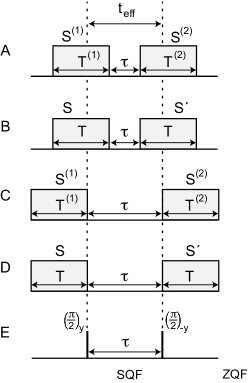
Figure 2: Characteristic families of Ramsey sequences are schematically represented. Sequences A-D consist of (rectangular, shaped or composite) pulses with finite maximum amplitude and finite durations (rectangles). The inter-pulse delays are denoted as $\tau$. The dashed vertical lines separated by the delay $t_{\it eff}=\tau+\delta$ mark the effective evolution time (cf. Eqs. (2) and (14)) of the Ramsey sequences. Sequence E shows the idealized Ramsey sequence, consisting of two ideal hard 90^∘ pulses with unlimited amplitudes and negligible durations and pulse phases $y$ and $-y$. After the first and the second pulse of all Ramsey sequences (A-E), an effective single quantum filter (SQF) and a zero quantum filter (ZQF) is applied.

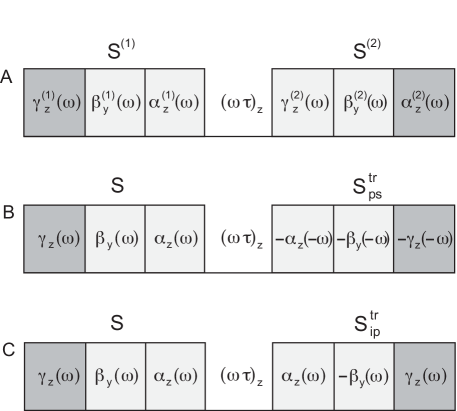
Figure 3: (A) Schematic representation of the effective rotations of a general Ramsey sequence $S^{(1)}$-$\tau$-$S^{(2)}$ in terms of the offset-dependent Euler angles of the pulses $S^{(1)}$ and $S^{(2)}$. In addition to the effective Euler rotations $\gamma_{z}^{(k)}(\omega)$, $\beta_{y}^{(k)}(\omega)$ and $\alpha_{z}^{(k)}(\omega)$ of the pulses $S^{(k)}$ with $k\in\{1,2\}$, the spins are subject to a rotation by the angle $\omega\tau$ around the $z$-axis during the delay $\tau$ between the pulses. The subscript ($y$ or $z$) of each rotation angle indicates the corresponding rotation axis and $\omega=2\pi\nu$ corresponds to the offset in angular frequency units. In addition, the corresponding transformations for the sequences $S$-$\tau$-$S^{\prime}$ are shown in (B) for the pulse $S^{\prime}=S^{\it tr}_{ps}$, which is a time-reversed version of the pulse $S$ with an additional phase shift by $\pi$, and in (C) for the pulse $S^{\prime}=S^{\it tr}_{ip}$, which is a time-reversed version of $S$ with inverted phase, cf. Table 1. The Euler angles $\gamma_{z}^{(1)}(\omega)$ and $\alpha_{z}^{(2)}(\omega)$ are irrelevant for the resulting Ramsey fringe pattern, which is indicated by darker boxes.

2.2 Ideal Ramsey pulse sequence

Fig. 2 E shows an idealized hard-pulse version of the Ramsey sequence, consisting of a $90^{\circ}_{y}$ pulse, a delay $\tau$ and a $90^{\circ}_{-y}$ pulse.

The initial Bloch vector is assumed to be oriented along the $z$-axis:

$${\bf M}(0)=\left(0,\ 0,\ 1\right)^{\rm T}$$ (3)

(The superscript "T" denotes the transpose of the row vector). The first hard pulse effects an instantaneous $90^{\circ}$ rotation of negligible duration around the $y$-axis, bringing the Bloch vector to the $x$-axis of the rotating frame. During the following delay $\tau$, the Bloch vector rotates around the $z$-axis with the offset frequency $\omega$, resulting in

$${\bf M(\tau)}=\left(\cos(\omega\tau),\ \sin(\omega\tau),\ 0\right)^{\rm T}.$$ (4)

The second pulse effects an instantaneous $90^{\circ}$ rotation around the $-y$-axis. This results in the final Bloch vector

$${\bf M^{\it final}}=\left(0,\ \sin(\omega\tau),\ \cos(\omega\tau)\right)^{\rm T}$$ (5)

with the $z$-component

$${M}_{z}^{\it final}=\rm cos(\omega\tau),$$ (6)

which in fact has the form of the target modulation defined in Eq. (1) (with $\delta=0$).

3 Ramsey sequences based on composite pulses with finite amplitude

In the following, we will use the generic term “pulse” for rectangular, composite or shaped pulses. Each pulse $S$ is characterized by its duration $T$, the time-dependent pulse amplitude $u(t)$ and the pulse phase $\xi(t)$. The pulse amplitude is commonly given in terms of the on-resonance Rabi frequency in units of Hz. Alternatively, the pulse field can be specified in terms of its $x$- and $y$-components $u_{x}(t)=u(t)\cos\xi(t)$ and $u_{y}(t)=u(t)\sin\xi(t)$. Here we analyze a general Ramsey experiment consisting of two pulses $S^{(1)}$ and $S^{(2)}$, separated by a delay $\tau$ (cf. Fig. 2 A, C and 3 A). It is always possible to represent the overall effect of each pulse $S^{(k)}$ (with $k\in\{1,\ 2\}$) by three Euler rotations $\gamma_{z}^{(k)}(\omega)$, $\beta_{y}^{(k)}(\omega)$, $\alpha_{z}^{(k)}(\omega)$, where the subscripts ($z$ or $y$) denote the (fixed) rotation axis [38, 39].

This is illustrated schematically in Fig. 3A. During the delay $\tau$ between the pulses, a spin with offset $\omega$ experiences an additional rotation by the angle $\omega\tau$ around the $z$-axis, which is represented as $(\omega\tau)_{z}$ in Fig. 3. Note that the Euler rotations $\gamma_{z}^{(1)}(\omega)$ and $\alpha_{z}^{(2)}(\omega)$ are irrelevant for Ramsey experiments, because the initial Bloch vector ${\bf M}(0)=(0,0,1)^{\rm T}$ is invariant under $\gamma^{(1)}_{z}$ and because $M_{z}^{\it final}$ is invariant under $\alpha^{(2)}_{z}$.

The remaining relevant rotations are $\beta_{y}^{(1)}(\omega)$ and $\alpha_{z}^{(1)}(\omega)$ for the first pulse, the rotation $(\omega\tau)_{z}$ for a spin with offset frequency $\omega$ during the delay $\tau$ and $\gamma_{z}^{(2)}(\omega)$ and $\beta_{y}^{(2)}(\omega)$ for the second pulse. In addition to these rotations, it is common practice in spectroscopy to eliminate any remaining $z$-component of the Bloch vector after the first pulse by a single quantum filter (SQF), because it would be invariant during the delay $\tau$ and hence cannot contribute to the desired $\tau$ dependence of $M_{z}^{\it final}$. For example, in 2D NMR spectroscopy, any remaining $z$-component results in unwanted "axial peaks" which can obscure the desired "cross peaks" in the final two-dimensional spectrum [1]. Similarly, as the experimenter is only interested in the $z$-component of the final magnetization, the remaining $x$- or $y$-components of the final Bloch vector can either be ignored or can be actively eliminated using a zero-quantum filter (ZQF) (or a $z$ filter) after the second pulse. In practice, single quantum filters and zero-quantum filters can e.g. be realized using phase cycles or so-called "homo-spoil" or "crusher" gradients [1, 3, 29]. Hence, the overall sequence of relevant transformations can be summarized schematically as:

$${\bf M}(0)=\left(\begin{array}[]{c}0\\ 0\\ 1\end{array}\right)\ \overset{\beta^{(1)}_{y}}{\longrightarrow}\ \ \overset{\alpha^{(1)}_{z}}{\longrightarrow}\ \ \overset{\bf SQF}{\longrightarrow}\ \ \overset{(\omega\tau)_{z}}{\longrightarrow}\ \ \overset{\gamma^{(2)}_{z}}{\longrightarrow}\ \ \overset{\beta^{(2)}_{y}}{\longrightarrow}\ \ \overset{\bf ZQF}{\longrightarrow}\ \left(\begin{array}[]{c}0\\ 0\\ M_{z}^{\it final}\end{array}\right).$$ (7)

A straightforward calculation yields the following expression for $M_{z}^{\it final}$ as a function of the offset frequency $\omega$, the delay $\tau$ and the Euler angles $\beta^{(1)}(\omega)$, $\alpha^{(1)}(\omega)$, $\gamma^{(2)}(\omega)$, $\beta^{(2)}(\omega)$:

$$M_{z}^{\it final}=-\sin\{\beta^{(1)}(\omega)\}\ \sin\{\beta^{(2)}(\omega)\}\ \cos\{\omega\tau+\alpha^{(1)}(\omega)+\gamma^{(2)}(\omega)\}.$$ (8)

For pulses $S^{(k)}$ with offset-independent Euler angles

$$\beta_{\it ideal}^{(1)}(\omega)=90^{\circ}\ \ \ \ {\rm and}\ \ \ \ \beta_{\it ideal}^{(2)}(\omega)=-90^{\circ},$$ (9)

the amplitude of the desired time-dependent cosine modulation (cf. Eq. (1)) of $M_{z}^{\it final}$ is maximized ($s_{R}=1$) and has the form

$$M_{z}^{\it final}=\cos\{\omega\tau+\alpha^{(1)}(\omega)+\gamma^{(2)}(\omega)\}.$$ (10)

Furthermore, we can decompose the offset-dependent Euler angles $\alpha^{(1)}(\omega)$ and $\gamma^{(2)}(\omega)$ in linear and nonlinear parts in the form

$$\alpha^{(1)}(\omega)=\omega R_{\alpha}^{(1)}T^{(1)}+\alpha^{(1)nl}(\omega)\ \ \ {\rm and}\ \ \ \gamma^{(2)}(\omega)=\omega R_{\gamma}^{(2)}T^{(2)}+\gamma^{(2)nl}(\omega),$$ (11)

with the relative slopes $R_{\alpha}^{(1)}$ and $R_{\gamma}^{(2)}$ [40] of the linear offset-dependence and the duration $T^{(k)}$ of pulse $S^{(k)}$, i.e. the nonlinear terms are given by

$$\alpha^{(1)nl}(\omega)=\alpha^{(1)}(\omega)-\omega R_{\alpha}^{(1)}T^{(1)}\ \ \ {\rm and}\ \ \ \gamma^{(2)nl}(\omega)=\gamma^{(2)}(\omega)-\omega R_{\gamma}^{(2)}T^{(2)}.$$ (12)

This allows us to express $M_{z}^{\it final}$ in the form

$$M_{z}^{\it final}=\cos\{\omega\tau+\omega R_{\alpha}^{(1)}T^{(1)}+\omega R_{\gamma}^{(2)}T^{(2)}+\alpha^{(1)nl}(\omega)+\gamma^{(2)nl}(\omega)\}$$ (13)

$$=\cos\{\omega t_{\it eff}+\alpha^{(1)nl}(\omega)+\gamma^{(2)nl}(\omega)\}\ \ \ \ \ \ \ \ \ \ \ \ \ \ \ \ \ \ \ \$$

with the offset-independent effective evolution time

$$t_{\it eff}=\tau+R_{\alpha}^{(1)}T^{(1)}+R_{\gamma}^{(2)}T^{(2)}.$$ (14)

Hence, if the nonlinear terms of the Euler angles $\alpha^{(1)}(\omega)$ and $\gamma^{(2)}(\omega)$ cancel in Eq. (13) for a pulse pair $S^{(1)}$ and $S^{(2)}$, i.e. if the condition

$$\alpha^{(1)nl}(\omega)+\gamma^{(2)nl}(\omega)\overset{!}{=}0$$ (15)

is satisfied, the modulation of the $z$-component of the final Bloch vector has the desired form of Eq. (1):

$$M_{z}^{\it final}(\tau)=\cos\{\omega(\tau+\delta)\}$$ (16)

with the fixed effective delay

$$\delta=R_{\alpha}^{(1)}T^{(1)}+R_{\gamma}^{(2)}T^{(2)}.$$ (17)

Note that according to Eq. (15) it is not necessary that the nonlinear terms of the individual Euler angles $\alpha^{(1)}(\omega)$ and $\gamma^{(2)}(\omega)$ are zero. Eq. (15) opens the possibility to design pairs of Ramsey pulses such that the nonlinear terms $\alpha^{(1)nl}(\omega)$ and $\gamma^{(2)nl}(\omega)$ cancel each other. Similarly, if $\delta=0$ is desired for a given application, according to Eq. (17) it is not necessary for the individual relative slopes $R_{\alpha}^{(1)}$ and $R_{\gamma}^{(2)}$ to be zero. As phase slopes can be positive or negative [40], it is possible to achieve $\delta=0$, even if the individual phase slopes are nonzero. As discussed in the introduction, the mutual compensation of pulse imperfections is expected to result in superior performance of s²-COOP pulses. In the next section, two equivalent approaches for the design of s²-COOP pulses for Ramsey sequences will be presented.

4 Optimization of s²-COOP pulses

4.1 Filter-based approach to s²-COOP pulse optimization

Pulse sequences are designed to result in coherence transfer functions [1] with a desired dependence on the system parameters such as resonance offsets or coupling constants, and on the delays between the pulses. It is important to realize that transfer functions are not only determined by the sequence of pulses but also by inserted filter elements that are typically realized in practice by pulsed field gradients or phase cycles [1, 29]. Depending on the chosen filter elements, the same sequence of pulses can result in very different transfer functions and hence very different spectroscopic information. For example, experiments such as NOESY [34, 1], relayed correlation spectroscopy [41] and double-quantum filtered correlation spectroscopy [42] use different filter elements and yield very different spectroscopic information although they are all based on a sequence of three 90^∘ pulses [29]. If terms of the density operator are filtered based on coherence order [1], the desired transfer function of a given pulse sequence is reflected by so-called coherence-order pathways [1] but more general filter criteria can also be used [44, 45].

Filters perform non-unitary transformations of the density operator and in general correspond to projections of the density operator to a subspace of interest. For example if the Ramsey sequence is applied to a two-level system, where the state of the system is completely described by the Bloch vector, a single quantum filter (SQF) is numerically simply implemented by setting the $z$-component of the Bloch vector to zero. In the GRAPE algorithm, filters can be treated in complete analogy to relaxation losses [15]: In each iteration, the Bloch vector ${\bf M}(t)$ (or in general the density operator) evolves forward in time, starting from a given initial state ${\bf M}(0)$ and also passes the filters forward in time. For a given final cost (quality factor) $\Phi$, the corresponding final costate vector [46, 15]

$${\lambda}_{f}=\left(\partial\Phi/\partial M_{x}(T_{f}),\ \partial\Phi/\partial M_{y}(T_{f}),\ \partial\Phi/\partial M_{z}(T_{f})\right)^{\rm T}$$ (18)

at the final time $T_{f}$ is evolved backward and also passes the filters backward in time. (Passing a filter backward in time has the same effect as passing it forward in time, e.g. a SQF sets the $z$-component of the Bloch vector to zero in both directions.) The evolution of $M(t)$ and $\lambda(t)$ is shown schematically in Fig. 4 A. With the known state and costate vectors $M(t)$ and $\lambda(t)$, the high-dimensional gradient of the final cost with respect to the control amplitudes can be efficiently calculated [46, 15, 18] in each iteration step. This gradient information can then be used to update the control parameters in each iteration until convergence is reached.

This procedure makes it possible to optimize the desired transfer function of an entire sequence of pulses such that they can compensate each other’s imperfections in the best possible way. The full flexibility of the available degrees of freedom is exploited by this approach, resulting in optimal s²-COOP pulses. Most notably, in this approach the number of pulses in a sequence is not limited.

In the case of the Ramsey sequence, for each offset $\omega$, the final figure of merit $\Phi^{(a)}(\omega)$ to be maximized can be defined in terms of the deviation of the $z$-component of the final Bloch vector ${\bf M}^{\it final}(\omega)={\bf M}(T_{f},\omega)$ from the target modulation ${\bf M}^{\it target}_{z}(\omega)$ defined in Eq. (1):

$$\Phi^{(a)}(\omega)=1-\{M_{z}^{\it final}(\omega)-M^{\it target}_{z}(\omega)\}^{2}$$ (19)

and according to Eq. (18), the final costate vector $\lambda^{(a)}_{f}$ is given by

$$\lambda^{(a)}_{f}(\omega)=2\left(0,\ 0,\ M^{\it target}_{z}(\omega)-M_{z}^{\it final}(\omega)\right)^{\rm T}=2\left(0,\ 0,\ \cos\{\omega(\tau+\delta)-M_{z}^{\it final}(\omega)\}\right)^{\rm T}.$$ (20)

Formally, in Eqs. (1), (8) and (16), the inter-pulse delay $\tau$ can also be chosen to be negative. If it is chosen to be $-\delta$ (and assuming $s_{R}=1$), this results in $M_{z}^{\it target}=1$. Hence, an alternative figure of merit can be defined simply as

$$\Phi^{(b)}(\omega)=M^{\it final}(\omega)\ \ {\rm for}\ \ \tau=-\delta,$$ (21)

which should be as large as possible and ideally should approach its maximum value of 1 for all offsets $\omega$. In this case, the final costate vector $\lambda^{(b)}_{f}$ is simply given by

$$\lambda^{(b)}_{f}(\omega)=\left(0,\ 0,\ 1\right)^{\rm T}.$$ (22)

(The two alternative offset-dependent quality factors $\Phi^{(a)}(\omega)$ and $\Phi^{(b)}(\omega)$ are closely related to the quality factors for individual pulses used in [47] and [46], respectively.)

In the GRAPE algorithm [15], the overall quality factor $\Phi$ of a given pulse sequence is defined as the average of the local quality factors over the offset range of interest and the gradient for the overall quality factor is simply the average of the offset dependent gradients. In complete analogy to variations in offsets, variations of the scaling factor of the control amplitude can be taken into account [15].

4.2 Symmetry-adapted approach to s²-COOP pulse optimization

Here an alternative, symmetry-adapted approach for the optimization of s²-COOP pulses is introduced. Although in the case of Ramsey pulses, this approach is equivalent to the filter-based approach discussed in the previous section, it is worthwhile to be considered as it provides a different perspective, which elucidates the inherent symmetry of the problem to design a pair of maximally cooperative Ramsey pulses. In order to prepare the detailed discussion of this approach, we briefly summarize the effects of time reversal, phase inversion and phase shift on the Euler angles associated with a given composite or shaped pulse $S$.

4.2.1 Effects of time reversal, phase inversion and phase shift by $\pi$

In order to understand the symmetry-adapted approach to s²-COOP pulses as well as the construction principles of Ramsey sequences based on the classes of pulses discussed in sections 6 and 7, it is helpful to consider how the Euler angles $\gamma(\omega)$, $\beta(\omega)$, and $\alpha(\omega)$ of a given pulse $S$ with duration $T$, amplitude $u(t)$ and phase $\xi(t)$ are related to the Euler angles $\gamma^{\prime}(\omega)$, $\beta^{\prime}(\omega)$, and $\alpha^{\prime}(\omega)$ of a modified pulse $S^{\prime}$. We consider the following three symmetry relations [48] (and combinations thereof) between $S$ and S^′:

$\bullet$ phase shift by $\pi$ (denoted as "ps")

$\bullet$ inversion of phase (denoted as "ip")

$\bullet$ time reversal of the pulse amplitude and phase (denoted as "tr")

The explicit definitions of these pulse modifications in terms of the time-dependent pulse amplitudes $u(t)$ and phases $\xi(t)$ are summarized in the second and third column of Table 1. In addition to the pulses $S_{ps}$, $S_{ip}$ and $S^{tr}$, Table 1 also includes the combinations $S_{ps}^{tr}$ and $S_{ip}^{tr}$ (and for completeness the original pulse $S$). For each of these pulse modifications, the relations between the Euler angles of $S^{\prime}$ and $S$ are summarized in the Table. Explicit derivations of these relations are provided in the Appendix. In addition, the relation between the Euler angles of a pulse $S$ and its inverse $S^{-1}$ is given in the last row of Table 1. Note that for non-zero offset frequencies $\omega$ none of the modified pulses $S_{ps}$, $S_{ip}$, $S^{tr}$, $S_{ps}^{tr}$ and $S_{ip}^{tr}$ is identical to the inverse $S^{-1}$ of the pulse. Either the order of the Euler angles, their algebraic signs or the sign of the offset frequency where they are evaluated are different. In particular, it is important to note that simply reversing the amplitude and phase of a pulse $S$ in time (yielding the pulse $S^{tr}$) does not correspond to $S^{-1}$, except for the on-resonance case $\omega=0$, where the detuning is zero. Hence the "time-resersed" pulse $S^{tr}$ does not have the same effect as a backward evolution in time. As shown in Table 1, the modified pulses $S_{ip}^{tr}$ and $S_{ps}^{tr}$ have the closest relation with $S^{-1}$: The time-reversed pulse with inverted phase $S_{ip}^{tr}$ has the same order of the Euler angles as $S^{-1}$ and they are also evaluated at the same offset frequency $\omega$, the only difference is the algebraic sign of the angles $\gamma$ and $\alpha$. This close relationship of $S_{ip}^{tr}$ and $S^{-1}$ is exploited in the symmetry-adapted analysis of Ramsey s²-COOP pulses in section 4.2.2.

The time-reversed pulse with a phase shift of $\pi$ ($S_{ps}^{tr}$) has the same order of the Euler angles and they have the same sign as for $S^{-1}$, but they are evaluated at the negative offset frequency $-\omega$. As will be shown below, $S_{ps}^{tr}$ pulses turn out to play a crucial role in the construction of s²-COOP pulses based on a special class of pulses (denoted as $ST$ pulses) that will be introduced and rigorously defined in section 6.

Table 1: Relations of pulse amplitude $u(t)$, pulse phase $\xi(t)$ and the offset-dependent Euler angles $\gamma(\omega)$, $\beta(\omega)$ and $\alpha(\omega)$ for symmetry-related pulses $S$ and $S^{\prime}$.

$S^{\prime}$	$u^{\prime}(t)$	$\xi^{\prime}(t)$	$\gamma^{\prime}(\omega)$	$\beta^{\prime}(\omega)$	$\alpha^{\prime}(\omega)$
$S$	$u(t)$	$\xi(t)$	$\gamma(\omega)$	$\beta(\omega)$	$\alpha(\omega)$
$S_{ps}$	$u(t)$	$\xi(t)+\pi$	$\gamma(\omega)$	$-\beta(\omega)$	$\alpha(\omega)$
$S_{ip}$	$u(t)$	$-\xi(t)$	$-\gamma(-\omega)$	$-\beta(-\omega)$	$-\alpha(-\omega)$
$S^{tr}$	$u(T-t)$	$\xi(T-t)$	$-\alpha(-\omega)$	$\beta(-\omega)$	$-\gamma(-\omega)$
$S^{tr}_{ps}$	$u(T-t)$	$\xi(T-t)+\pi$	$-\alpha(-\omega)$	$-\beta(-\omega)$	$-\gamma(-\omega)$
$S^{tr}_{ip}$	$u(T-t)$	$-\xi(T-t)$	$\alpha(\omega)$	$-\beta(\omega)$	$\gamma(\omega)$
$S^{-1}$	-	-	$-\alpha(\omega)$	$-\beta(\omega)$	$-\gamma(\omega)$

ps: phase shifted by $\pi$, ip: inverted phase, tr: time reversal

4.2.2 Designing s²-COOP Ramsey pulses by the simultaneous optimization of excitation pulses

In the Ramsey scheme, the two pulses appear to have quite different tasks. A more symmetric picture emerges if the effect of the second pulse is effectively analyzed backward in time.

For a given second Ramsey pulse $S^{(2)}$ (with Euler angles $\gamma^{(2)}(\omega)$, $\beta^{(2)}(\omega)$, and $\alpha^{(2)}(\omega)$), let us consider the pulse $\tilde{S}^{(2)}$ (with Euler angles $\tilde{\gamma}^{(2)}(\omega)$, $\tilde{\beta}^{(2)}(\omega)$, and $\tilde{\alpha}^{(2)}(\omega)$), which we define as the time-reversed version of $S^{(2)}$ with inverted phase:

$$\tilde{S}^{(2)}=(S^{(2)})^{tr}_{ip}\ \ \ {\rm and\ conversely\ \ \ }S^{(2)}=(\tilde{S}^{(2)})^{tr}_{ip}.$$ (23)

Using the relations of the Euler angles between a pulse and its time-reverse and phase-inverted version from Table 1, we find

$$\gamma^{(2)}(\omega)=\tilde{\alpha}^{(2)}(\omega),\ \ \ \ \ \beta^{(2)}(\omega)=-\tilde{\beta}^{(2)}(\omega),\ \ \ \ \ \alpha^{(2)}(\omega)=\tilde{\gamma}^{(2)}(\omega).$$ (24)

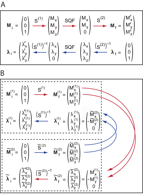
Figure 4: In panel A, the forward evolution of the Bloch vector $M(t)$ and the backward evolution of the costate vector $\lambda(t)$ for the filter-based s²-COOP pulse optimization (cf. section 4.1) are shown for a general Ramsey sequence $S^{(1)}$-$\tau$-$S^{(2)}$. Panel B illustrates the evolution of the Bloch and costate vectors that are considered in the symmetry-adapted approach for the simultaneous optimization of the two pulses $S^{(1)}$ and $\tilde{S}^{(2)}$, see Eq. (23) (cf. section 4.2).

Special case without auxiliary effective delay ($\delta=0$): For simplicity, we first consider the special case where the effective evolution time $t_{\it eff}$ is identical to the inter-pulse delay $\tau$, which is the case if the auxiliary fixed effective delay $\delta$ is zero (cf. Fig. 2 C). Based on the general analysis of the Ramsey sequence in section 3 (cf. Eqs. (9) and (10)), this case corresponds to the following conditions for the Euler angles of the second pulse:

$$\gamma^{(2)}(\omega)=-\alpha^{(1)}(\omega),\ \ \ \ \ \beta^{(2)}(\omega)=-\pi/2,\ \ \ \ \ \alpha^{(2)}(\omega):{\rm arbitrary}.$$ (25)

Using the relations (24), these conditions translate into the following conditions for pulse $\tilde{S}^{(2)}$:

$$\tilde{\gamma}^{(2)}(\omega):{\rm arbitrary}\ \ \ \ \ \tilde{\beta}^{(2)}(\omega)=\pi/2,\ \ \ \ \ \tilde{\alpha}^{(2)}(\omega)=-\alpha^{(1)}(\omega).$$ (26)

Hence, the two pulses $S^{(1)}$ and $\tilde{S}^{(2)}$ play completely symmetric roles. Both have arbitrary first Euler angles ($\gamma^{(1)}(\omega)$ and $\tilde{\gamma}^{(2)}(\omega)$), the second Euler angles ($\beta^{(1)}(\omega)$ and $\tilde{\beta}^{(2)}(\omega)$) should both be 90^∘ and the third Euler angles ($\alpha^{(1)}(\omega)$ and $\tilde{\alpha}^{(2)}(\omega)$) can have an arbitrary offset dependence, provided that for each offset frequency $\omega$ they have the same magnitude but opposite algebraic signs, cf. Eq. (26). The initial Bloch vector ${\bf M}_{i}^{(1)}=\left(0,\ 0,\ 1\right)^{\rm T}$ is transferred by the pulse $S^{(1)}$ and a subsequent single quantum filter to

$${\bf M}_{i}^{(1)}\ \overset{\gamma^{(1)}_{z}}{\longrightarrow}\ \ \overset{\beta^{(1)}_{y}}{\longrightarrow}\ \ \overset{\alpha^{(1)}_{z}}{\longrightarrow}\ \ \overset{\bf SQF}{\longrightarrow}\ {\bf M}_{f}^{(1)}=\left(\sin{\beta^{(1)}}\cos{\alpha^{(1)}},\ \sin{\beta^{(1)}}\sin{\alpha^{(1)}},\ 0\right)^{\rm T}.$$ (27)

Starting from the same initial Bloch vector ${\bf M}_{i}^{(2)}={\bf M}_{i}^{(1)}$, the pulse $\tilde{S}^{(2)}$ and a subsequent zero quantum filter yields

$${\bf\tilde{M}}^{(2)}_{i}\ \overset{\tilde{\gamma}^{(2)}_{z}}{\longrightarrow}\ \ \overset{\tilde{\beta}^{(2)}_{y}}{\longrightarrow}\ \ \overset{\tilde{\alpha}^{(2)}_{z}}{\longrightarrow}\ \ \overset{\bf SQF}{\longrightarrow}\ {\bf\tilde{M}}_{f}^{(2)}=\left(\sin{\tilde{\beta}^{(2)}}\cos{\tilde{\alpha}^{(2)}},\ \sin{\tilde{\beta}^{(2)}}\sin{\tilde{\alpha}^{(2)}},\ 0\right)^{\rm T}.$$ (28)

Ideally, the two final vectors ${\bf M}_{f}^{(1)}(\omega)$ and ${\bf\tilde{M}}_{f}^{(2)}(\omega)$ are both located in the transverse plane and have phase angles ${\alpha^{(1)}(\omega)}$ and ${\tilde{\alpha}^{(2)}(\omega)}$, respectively. According to the condition $\tilde{\alpha}^{(2)}(\omega)=-\alpha^{(1)}(\omega)$ (cf. Eq. (26)), the two vectors should be collinear if one of them is reflected about the $x$-axis. Hence, a figure of merit for the efficiency of the corresponding pair of s²-COOP Ramsey pulses can be defined as the scalar product of ${\bf M}_{f}^{(1)}(\omega)$ and the vector resulting from ${\bf\tilde{M}}_{f}^{(2)}(\omega)$ if the sign of its $y$-component is inverted:

$$\Phi^{(c)}(\omega)=\left(M^{(1)}_{f,x},\ M^{(1)}_{f,y},\ 0\right)\left(\tilde{M}^{(2)}_{f,x},\ -\tilde{M}^{(2)}_{f,y},\ 0\right)^{\rm T}=M^{(1)}_{f,x}\tilde{M}^{(2)}_{f,x}-M^{(1)}_{f,y}\tilde{M}^{(2)}_{f,y}.$$ (29)

With this quality factor, the control task to design a sequence of s²-COOP Ramsey pulses can be formulated as the concurrent optimization of two excitation pulses $S^{(1)}$ and $\tilde{S}^{(2)}$. The two identical initial state vectors ${\bf M}^{(1)}_{i}$ and ${\bf\tilde{M}}^{(2)}_{i}$ (cf. Eqs. (27) and (28)) diverge as they evolve forward in time under the action of the two different pulses $S^{(1)}$ and $\tilde{S}^{(2)}$. Based on Eqs. (18) and (29), the two costate vectors associated with ${\bf M}^{(1)}(t)$ and ${\bf\tilde{M}}^{(2)}(t)$ are given by

$${\bf\lambda}^{(1)}_{f}=\left(\tilde{M}^{(2)}_{f,x},\ -\tilde{M}^{(2)}_{f,y},\ 0\right)^{\rm T}\ \ \ \ {\rm and}\ \ \ \ {\bf\tilde{\lambda}}^{(2)}_{f}=\left(M^{(1)}_{f,x},\ -M^{(1)}_{f,y},\ 0\right)^{\rm T},$$ (30)

respectively. Following the steps of the standard GRAPE algorithm, the final costate vector ${\bf\lambda}^{(1)}_{f}$ is propagated backward in time under the action of the pulse $S^{(1)}$ and ${\bf\lambda}^{(2)}_{f}$ is propagated backward in time under the action of the pulse $\tilde{S}^{(2)}$. Thus separate gradients of $\Phi^{(c)}(\omega)$ are obtained with respect to the pulse sequence parameters of $S^{(1)}$ and $\tilde{S}^{(2)}$ [15, 28]. Note that the optimizations of $S^{(1)}$ and $\tilde{S}^{(2)}$ are not independent. In fact they are intimately connected as according to Eq. (30) the final costate vector after pulse $S^{(1)}$ depends on the $x$ and $y$ coordinates of the final Bloch vector for pulse $\tilde{S}^{(2)}$ and vice versa. This is represented graphically in Fig. 4 B by the curved arrows. Fig. 4 also illustrates the close kinship between the optimization of the Ramsey sequence based on $\Phi^{(b)}$ (cf. Eq. (21)) (shown schematically in Fig. 4 A) and the simultaneous optimizations of the excitation pulses $S^{(1)}$ and $\tilde{S}^{(2)}$ based on $\Phi^{(c)}$ (cf. Eq. (29)) (Fig. 4 B) for the special case $\delta=0$. Essentially, the evolution of ${\bf M}(t)$ is folded back after the zero quantum filter ZQF between the pulses: The first part of the entire forward evolution of the Bloch vector ${\bf M}(t)$ in Fig. 4 A (i.e. the evolution of ${\bf M}(t)$ under the pulse $S^{(1)}$ up to the zero quantum filter ZQF) corresponds to the forward evolution of ${\bf M}^{(1)}(t)$ under $S^{(1)}$ in Fig. 4 B. The second part of the forward evolution of ${\bf M}(t)$ in Fig. 4 A (i.e. the evolution of ${\bf M}(t)$ under the pulse $\tilde{S}^{(2)}$ starting from the ZQF) corresponds in Fig. 4 B to the backward evolution of ${\bf\tilde{\lambda}}^{(2)}(t)$ under $\tilde{S}^{(2)}$. Similarly, the backward evolution ${\bf\lambda}(t)$ in Fig. 4 A is folded back in Fig. 4 B. The change of sign of the $y$-components when going from ${\bf M}_{f}^{(1)}$ to ${\bf\tilde{\lambda}}_{f}^{(2)}$ and from ${\bf\tilde{M}}_{f}^{(2)}$ to ${\bf\lambda}_{f}^{(1)}$ (cf. curved arrows in Fig. 4 B) is a result of the construction of the pulse $\tilde{S}^{(2)}=(S^{(2)})^{tr}_{ip}$. In fact the two approaches are fully equivalent and the resulting gradients are identical.

General case, where the auxiliary effective delay $\delta$ can be non-zero: The symmetry-adapted approach outlined above for the special case of $\delta=0$ can be generalized for auxiliary non-vanishing constant effective evolution periods $\delta$ (cf. Fig. 2 A). Whereas for $\delta=0$ the Bloch vectors ${\bf M}_{f}^{(1)}$ and ${\bf\tilde{M}}_{f}^{(2)}$ should be related by a reflection about the $x$-axis independent of the offset $\omega$, for $\delta\neq 0$ they should be related by a reflection about an axis in the transverse plane that forms an angle $(\omega\delta)$ with the $x$-axis. In this case, the quality factor $\Phi^{(c)}(\omega)$ generalizes to

$$\Phi^{(d)}(\omega)=\{M^{(1)}_{f,x}\tilde{M}^{(2)}_{f,x}-M^{(1)}_{f,y}\tilde{M}^{(2)}_{f,y}\}\cos(\omega\delta)+\{M^{(1)}_{f,x}\tilde{M}^{(2)}_{f,y}+M^{(1)}_{f,y}\tilde{M}^{(2)}_{f,x}\}\sin(\omega\delta).$$ (31)

and hence in the GRAPE algorithm the corresponding final costate vectors resulting from Eqs. (18) and (31) ${\bf\lambda}^{(1)}_{f}$ and ${\bf\tilde{\lambda}}^{(2)}_{f}$ are given by

$${\bf\lambda}^{(1)}_{f}=\left(\tilde{M}^{(2)}_{f,x}\cos(\omega\delta)+\tilde{M}^{(2)}_{f,y}\sin(\omega\delta),\ \tilde{M}^{(2)}_{f,x}\sin(\omega\delta)-\tilde{M}^{(2)}_{f,y}\cos(\omega\delta),\ 0\right)$$ (32)

and

$$\tilde{\bf\lambda}^{(2)}_{f}=\left(M^{(1)}_{f,x}\cos(\omega\delta)+M^{(1)}_{f,y}\sin(\omega\delta),\ M^{(1)}_{f,x}\sin(\omega\delta)-M^{(1)}_{f,y}\cos(\omega\delta),\ 0\right).$$ (33)

As the symmetry-adapted approach to s²-COOP Ramsey pulses yields the optimized pulses $S^{(1)}$ and $\tilde{S}^{(2)}$, the pulse $S^{(1)}$ can be directly used as the first pulse in the Ramsey sequence, whereas the second pulse in the Ramsey sequence is $S^{(2)}=(\tilde{S}^{(2)})^{tr}_{ip}$ (cf. Eq. (23)). The optimized s²-COOP pulses $S^{(1)}$ and $S^{(2)}$ presented in the following were developed using the GRAPE algorithm based on the general Ramsey s²-COOP quality factor $\Phi^{(d)}(\omega)$.

5 Examples of s²-COOP Ramsey pulses

In order to illustrate the power of simultaneously optimized cooperative Ramsey pulses for realistic parameters, a challenging problem of practical interest was chosen from the field of two-dimensional (2D) NMR spectroscopy. The 2D NOESY experiment [34, 1], which is widely used to measure inter-nuclear distances for the structure elucidation of molecules in solution, contains a frequency labeling block which is identical to the Ramsey sequence. (In the NOESY sequence, the effective evolution time $t_{\it eff}$ between the two Ramsey pulses is called the evolution period $t_{1}$.)

To facilitate the comparison of the relative magnitudes of the achievable bandwidth of a pulse with the maximum control amplitude (which is commonly stated in terms of the corresponding Rabi frequency in units of Hz), in the following we will discuss detunings in terms of the offset frequencies $\nu=\omega/(2\pi)$. As pointed out in the introduction, simple rectangular pulses cover only a bandwidth $\Delta\nu$ which is in the order of $2u^{max}$, where the bandwidth $\Delta\nu=\nu_{max}-\nu_{min}$ is defined as the difference between the largest and smallest offset frequencies (in units of Hz) with acceptable performance. For example, in high-resolution ¹³C-NMR spectroscopy, the maximum available control amplitude $u^{max}$ is typically in the order of 10 kHz, corresponding to a duration of a rectangular 90^∘ pulse of $T^{(90^{\circ})}=1/(4u^{max})=25\ \mu$s. With this amplitude, rectangular pulses only cover a bandwidth of about 20 kHz (corresponding to maximal or minimal detunings of about $\pm 10$ kHz). However, for currently developed NMR spectrometers with magnetic fields of up to 30 Tesla, a bandwidth $\Delta\nu=70$ kHz will be required in order to cover the typical chemical shift range of ¹³C spins in proteins. Hence, for high-field 2D ¹³C-¹³C-NOESY experiments [35] the bandwidth of the Ramsey-type frequency labeling building block should be up to seven times larger than $u^{max}$.

For this setting, pulses $S^{(1)}$ and $S^{(2)}$ were optimized simultaneously using the GRAPE algorithm based on the quality factor $\Phi^{(d)}$ (Eq. (31)). In addition to robustness with respect to offset frequencies of up to $\pm 3.5u^{max}$, the s²-COOP Ramsey pulses were also optimized to be robust with respect to scaling factors of the control amplitude between 0.95 and 1.05, corresponding to variations of $\pm 5\%$ relative to the nominal control amplitude due to pulse miscalibrations and spatial rf inhomogeneity. For simplicity, both pulses $S^{(1)}$ and $S^{(2)}$ were assumed to have identical pulse durations

$$T^{(1)}=T^{(2)}=T.$$ (34)

The pulses were digitized in steps of 0.5 $\mu$s. In the optimizations and the subsequent analysis, the overall performance of a given Ramsey sequence is quantified by the total quality factor

$$\Phi=\overline{\Phi^{(d)}(\omega)},$$ (35)

which is the average of $\Phi^{(d)}$ (cf. Eq. (31)) over the specified range of offset frequencies and scaling factors of the control amplitude.

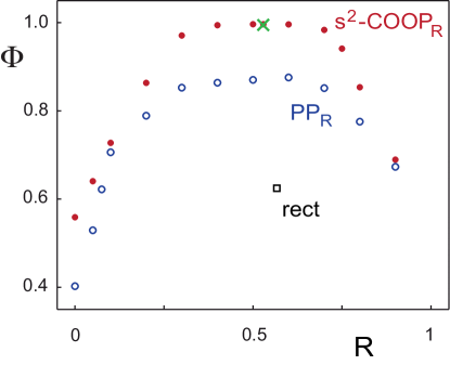
Figure 5: The maximum Ramsey quality factors $\Phi$ (cf. Eq. (35)) are shown as a function of the parameter $R$ (cf. Eq. (36)), which is proportional to the auxiliary delay $\delta$ (cf. Eq. (37)), for s²-COOP_R pulses (solid circles) and for PP_R pulses (open circles) with pulse durations of $T=75\ \mu$s and with a maximum pulse amplitude $u^{max}=10$ kHz. In addition, the quality factor $\Phi$ is shown for Ramsey sequences based on the saturation pulse (cross) discussed in section 6.1 and for simple rectangular 90^∘pulses with a duration of $25$ $\mu$s (open square).

For fixed pulse durations of $T=75\ \mu$s (which is only three times longer than the duration of a rectangular $90^{\circ}$ pulse for $u^{max}=10$ kHz), Fig. 5 shows the maximum total quality factors $\Phi$ for s²-COOP Ramsey pulses (solid circles) as a function of the parameter

$$R={{R_{\alpha}^{(1)}T^{(1)}+R_{\gamma}^{(2)}T^{(2)}}\over{T^{(1)}+T^{(2)}}}={{R_{\alpha}^{(1)}+R_{\gamma}^{(2)}}\over{2}},$$ (36)

where the last equality results from Eq. (34). Optimizations were performed for values of $R$ between 0 and 0.9, which are directly related to the durations of auxiliary constant effective delays

$$\delta=2RT$$ (37)

(cf. Eq. (17)). The quality factor reaches a plateau with $\Phi\approx 1$ between approximately $R=0.3$ and $R=0.7$, corresponding to an effective delay $\delta$ between 45 and 105 $\mu$s. A maximum quality factor of $\Phi=0.9965$ was found for $R=0.53$. The quality factor decreases markedly as $R$ approaches 0 or 1. For $R=0$, the auxiliary delay $\delta$ is zero. When $R$ approaches a value of 1, the effective delay $\delta$ approaches $2T=150\ \mu$s, i.e. it becomes as long as the total duration of the two pulses $S^{(1)}$ and $S^{(2)}$. For $R\leq 0.6$, all optimized s²-COOP pulses with a duration of $T=75\ \mu$s have a constant amplitude of $u(t)=u^{max}=10$ kHz, i.e. they fully exploit the maximal rf amplitude and the phase $\xi(t)$ of the pulses is smoothly modulated.

Figure 6: Shapes $u_{x}(t)$ and $u_{y}(t)$ of optimized s²-COOP_R (A) and PP_R (B) pulses with $R=0.53$, for simple rectangular 90${}_{\pm y}^{\circ}$ pulses (C) and PP₀ pulses (D). For a maximum pulse amplitude $u^{max}$ of 10 kHz, the duration of the rectangular 90^∘ pulse is 25 $\mu$s (C) and 75 $\mu$s for the remaining pulses (A, B, D). The effective evolution time $t_{\it eff}$ is 85 $\mu$s and with the auxiliary delays $\delta=79.5$ $\mu$s (A, B), 32 $\mu$s (C) and 0 $\mu$s (D) (cf. Eq. (37)), the corresponding inter-pulse delays $\tau$ are 5.5 $\mu$s (A, B), 53 $\mu$s (C) and 85 $\mu$s, respectively.

For example, Fig. 6 A shows the components $u_{x}(t)$ and $u_{y}(t)$ of the s²-COOP pulses $S^{(1)}$ and $S^{(2)}$ for $R=0.53$ (with $\Phi=0.9965$). A closer inspection of this figure reveals an a priori unexpected symmetry relation between the two pulses: $u_{x}^{(2)}$ is a time-reversed copy of $-u_{x}^{(1)}$ and $u_{y}^{(2)}$ is a time-reversed copy of $-u_{y}^{(1)}$. Hence the pulse $S^{(2)}$ can be obtained from $S^{(1)}$ by time-reversal and an additional phase shift by $\pi$, i.e. $S^{(1)}$ and $S^{(2)}$ have the surprising property

$$S^{(2)}\approx(S^{(1)})^{tr}_{ps}$$ (38)

(cf. Table 1). For the given parameters and constraints, almost all optimized s²-COOP pulses have this special symmetry relation, which was not explicitly imposed in the optimizations.

This finding raises the intriguing question why this particular symmetry relation plays such a prominent role for s²-COOP Ramsey pulse pairs. A detailed analysis is given in the next section. This analysis led to the discovery and characterization of a powerful new class of pulses (denoted as $ST$ pulses in the following), which makes it possible to closely approach the excellent performance of simultaneously optimized cooperative Ramsey pulses by a sequence consisting of the pulses $S^{(1)}=S^{ST}$ and $S^{(2)}=(S^{ST})^{tr}_{ps}$. A quantitative comparison of the performance of s²-COOP and ST pulses with the performance of conventional classes of individually optimized pulses in Ramsey sequences will be presented in section 7.

6 Analysis of Ramsey experiments based on pulse pairs with characteristic symmetry relations

Here we consider constructions of Ramsey sequence $S^{(1)}$-$\tau$-$S^{(2)}$ with $S^{(1)}=S$ and $S^{(2)}=S^{\prime}$, where $S^{\prime}$ can either be identical to $S$ or can be one of the symmetry related pulses $S_{ps}$, $S_{ip}$, $S^{tr}$, $S_{ps}^{tr}$ or $S_{ip}^{tr}$ discussed in in section 4.2.2. As shown in sections 1.2 and 3, the desired Ramsey fringe pattern can be expressed in the form of Eq. (1), with a constant auxiliary delay $\delta$, provided that condition (15) is fulfilled, which reduces here to

$$\alpha^{nl}(\omega)+\{\gamma^{\prime}\}^{nl}(\omega)\overset{!}{=}0,$$ (39)

where $\alpha^{nl}$ and $\{\gamma^{\prime}\}^{nl}$ are the nonlinear terms of the offset-dependent Euler angles $\alpha$ and $\gamma^{\prime}$ of the pulses $S$ and $S^{\prime}$, respectively (cf. Eqs. (11)-(12)).

For the sequence $S$-$\tau$-$S^{\prime}$, the general expression for $\delta$ given in Eq. (17) is reduces to

$$\delta=R_{\alpha}T+R_{\gamma^{\prime}}T,$$ (40)

where $R_{\alpha}$ and $R_{\gamma^{\prime}}$ are the relative slopes of the linear parts of the offset-dependent Euler angles $\alpha(\omega)$ and $\gamma^{\prime}(\omega)$ of the pulses $S$ and $S^{\prime}$, respectively (cf. Eq. (11)). With the relations between the Euler angles of $S$ and $S^{\prime}$ summarized in Table 1, the delay $\delta$ for the sequence $S$-$\tau$-$S^{\prime}$ can be expressed entirely in terms of the relative slopes $R_{\alpha}$ and $R_{\gamma}$ and the pulse duration $T$ of pulse $S$. For all considered types of symmetry related pulses $S^{\prime}$, the resulting expressions for $\delta$ are summarized in the second column of Table 2. Similarly, using the relations between the Euler angles of $S$ and $S^{\prime}$ (cf. Table 1), condition (39) can be expressed entirely in terms of the nonlinear terms $\alpha^{nl}$ and $\gamma^{nl}$ of the Euler angles $\alpha$ and $\gamma$ of the pulse $S$ (cf. Table 2).

Table 2: Summary of effective delay $\delta$, the Ramsey conditions for the Euler angles $\gamma$ and $\alpha$ of pulse $S$. and the scaling factor $s_{R}$ for the Ramsey fringe pattern created by the sequence $S$-$\tau$-$S^{\prime}$

$S^{\prime}$	$\delta$	Ramsey condition	$s_{R}$
$S$	$(R_{\alpha}+R_{\gamma})T$	$\alpha^{nl}(\omega)\overset{!}{=}-\gamma^{nl}(\omega)$	$-1$
$S_{ps}$	$(R_{\alpha}+R_{\gamma})T$	$\alpha^{nl}(\omega)\overset{!}{=}-\gamma^{nl}(\omega)$	$1$
$S_{ip}$	$(R_{\alpha}+R_{\gamma})T$	$\alpha^{nl}(\omega)\overset{!}{=}\gamma^{nl}(-\omega)$	$1$
$S^{tr}$	$2R_{\alpha}T$	$\alpha^{nl}(\omega)\overset{!}{=}\alpha^{nl}(-\omega)$	$-1$
$S^{tr}_{ps}$	$2R_{\alpha}T$	$\alpha^{nl}(\omega)\overset{!}{=}\alpha^{nl}(-\omega)$	$1$
$S^{tr}_{ip}$	$2R_{\alpha}T$	$\alpha^{nl}(\omega)\overset{!}{=}0\ \ \ \ \ \ \ \ \$	$1$
$S^{-1}$	0	-	$1$

For the cases $S^{\prime}=S$ and $S^{\prime}=S_{ps}$, the Euler angle $\gamma^{\prime}(\omega)$ is identical to $\gamma(\omega)$ and condition (39) reduces to $\alpha^{nl}(\omega)+\gamma^{nl}(\omega)\overset{!}{=}0$, i.e.

$$\alpha^{nl}(\omega)\overset{!}{=}-\gamma^{nl}(\omega).$$ (41)

For the case $S^{\prime}=S_{ip}$, $\gamma^{\prime}(\omega)=-\gamma(-\omega)$ and condition (39) reduces to $\alpha^{nl}(\omega)-\gamma^{nl}(-\omega)\overset{!}{=}0$, i.e.

$$\alpha^{nl}(\omega)\overset{!}{=}\gamma^{nl}(-\omega).$$ (42)

Hence for the cases without time reversal, where $S^{\prime}\in\{S$, $S_{ps}$, $S_{ip}\}$, condition (39) corresponds to a condition involving both Euler angles $\alpha$ and $\gamma$. In contrast, for pulses with time reversal, where $S^{\prime}\in\{$$S^{tr}$, $S^{tr}_{ps}$, $S^{tr}_{ip}\}$, condition (39) only involves the (nonlinear part of) the Euler angle $\alpha(\omega)$, i.e. the performance of the Ramsey sequence $S$-$\tau$-$S^{\prime}$ is completely independent of $\gamma(\omega)$. For example, for $S^{\prime}=S^{tr}_{ip}$ (cf. Table 1 and Fig. 3 C) we find $\gamma^{\prime}(\omega)=\alpha(\omega)$ and condition (39) reduces to $\alpha^{nl}(\omega)+\alpha^{nl}(\omega)=2\alpha^{nl}(\omega)\overset{!}{=}0$, i.e.

$$\alpha^{nl}(\omega)\overset{!}{=}0.$$ (43)

Hence for high-fidelity Ramsey sequences with $S^{\prime}=S^{tr}_{ip}$, only pulses with a negligible nonlinear offset dependence of the Euler angle $\alpha(\omega)$ are suitable. This condition is fulfilled by universal rotation (UR) pulses [49, 20] and point-to-point (PP_R) pulses either with $\alpha(\omega)=0$ (corresponding to $R=R_{\alpha}=0$, cf. Eq. (60)) or so-called Iceberg pulses [40] with $\alpha(\omega)=R_{\alpha}T$ (with $R=R_{\alpha}\neq 0$ (cf. discussion in section 7.1).

However, a very different situation emerges for Ramsey sequences with $S^{\prime}=S^{tr}$ or for $S^{\prime}=S^{tr}_{ps}$ (cf. Table 1 and Fig. 3 B). In this case, $\gamma^{\prime}(\omega)=-\alpha(-\omega)$ and condition (39) reduces to $\alpha^{nl}(\omega)-\alpha^{nl}(-\omega)\overset{!}{=}0$, i.e. to the condition

$$\alpha^{nl}(\omega)\overset{!}{=}\alpha^{nl}(-\omega).$$ (44)

Hence for $S^{\prime}=S^{tr}$ and $S^{\prime}=S^{tr}_{ps}$, it is sufficient for the nonlinear term of $\alpha^{nl}(\omega)$ to have a symmetric offset dependence but $\alpha^{nl}(\omega)$ is not required to be zero. Only its anti-symmetric component

$$\alpha^{nl}_{a}(\omega)={{\alpha^{nl}(\omega)-\alpha^{nl}_{s}(\omega)}\over{2}}$$ (45)

has to vanish, i.e. condition (44) is equivalent to

$$\alpha^{nl}_{a}(\omega)\overset{!}{=}0.$$ (46)

Compared to Eq. (44), this significantly less restrictive condition suggests that constructions of Ramsey sequences with $S^{\prime}=S^{tr}$ or $S^{\prime}=S^{tr}_{ps}$ offer a decisive advantage compared to other constructions. In fact, this is borne out by the results of s²-COOP pulse optimizations without any symmetry constraints presented in section 5, which are almost exclusively of the form $S$-$\tau$-$S^{\prime}$ with $S^{tr}_{ps}$.

If the conditions specified for each of the Ramsey constructions summarized in Table 2 (including $\beta(\omega)=90^{\circ}$, cf. condition (9)) are satisfied, the sequences create the desired fringe pattern defined in Eq. (1).

Based on Eq. (8) and the relations between $\beta(\omega)$ and $\beta^{\prime}(\omega)$ summarized in Table 1, it is straightforward to show that the algebraic sign of the scaling factor $s_{R}$ depends on the pulse type $S^{\prime}$, as indicated in the last column of Table 2. For the special cases $S^{\prime}=S$ and $S^{\prime}=S^{tr}$, the scaling factor is $s_{R}=-1$, whereas for the remaining cases $s_{R}=1$. For practical applications, the sign of $s_{R}$ is irrelevant, as it is always possible to correct for it by simply multiplying the detected signal by $s_{R}$. The fact that in section 5 only pulse sequences with $S^{\prime}=S^{tr}_{ps}$ but no pulse sequences with $S^{\prime}=S^{tr}$ were found is a simple consequence of the different algebraic signs of the scaling factor $s_{R}$ for their Ramsey fringe pattern (cf. Table 2) and the choice $s_{R}=1$ for the target pattern in the optimizations.

Because of its importance, in the next section a novel class of pulses will be formally defined based on (44) and an efficient algorithm for their direct numerical optimization will be presented.

6.1 Broadband ST pulses: symmetric offset dependence of the Euler angle $\alpha$ with an optional tilt

We define the class of ST${}_{R}(\beta_{0})$ pulses based on the following three properties of their offset-dependent Euler angles (cf. Table 3).

Definition of ST${}_{R}(\beta_{0})$ pulses:

(a) It is required that the offset-dependent Euler angle $\alpha(\omega)$ can be expressed in the form

$$\alpha(\omega)\overset{!}{=}\omega RT+\alpha_{s}(\omega),$$ (47)

where $\omega RT$ is the part of $\alpha(\omega)$ that is linear in $\omega$, $R=R_{\alpha}$ is the relative slope of this linear part [40] and

$$\alpha_{s}(\omega)={{\alpha(\omega)+\alpha(-\omega)}\over{2}}$$ (48)

is the symmetric part of $\alpha(\omega)$.

(b) The Euler angle $\beta(\omega)$ is required to have the offset-independent value

$$\beta(\omega)\overset{!}{=}\beta_{0}.$$ (49)

(c) The Euler angle $\gamma(\omega)$ can have an arbitrary offset-dependence, i.e. it is not restricted.

Note that Eq. (47) in condition (a) is fully equivalent to Eqs. (44) and (46) (cf. Eq. (11)) as the symmetric part of $\alpha(\omega)$ is identical to the symmetric nonlinear part of $\alpha(\omega)$, because the linear term $\omega RT$ is anti-symmetric in $\omega$. Of course for a finite range of offset frequencies $\omega$, ST${}_{R}(\beta_{0})$ pulses can only be approximated in practice. In the context of Ramsey-type pulse sequences, we focus on the special case where $\beta_{0}=90^{\circ}$ (cf. Eq. (9)) and for the sake of simplicity, we will use the short form "ST_R" (or simply "ST") for "ST${}_{R}(90^{\circ})$" in the following. For a vanishing relative slope $R=0$, Eq. (47) implies that the offset-dependence of $\alpha(\omega)$ ist strictly symmetric. However, for a non-vanishing relative slope $R\neq 0$, the symmetric offset-dependence of $\alpha(\omega)$ is tilted and the acronym "ST" stands for symmetric offset dependence of the Euler angle $\alpha$ with an optional tilt.

Figure 7: Panel A shows the offset dependence of the Euler angle $\alpha(\nu)$ for an optimized ST_R pulse with $R=0.53$. The dashed line represents the linear part $\omega RT=2\pi\nu RT$ of $\alpha(\nu)$. Subtracting $\omega RT$ from $\alpha(\omega)$ yields the nonlinear part $\alpha^{nl}(\nu)$ (cf. Eq. (50)), which is shown in panel B. Panel C displays the small anti-symmetric nonlinear part $\alpha_{a}^{nl}(\nu)$ that remains if the symmetric nonlinear part $\alpha_{s}^{nl}(\omega)$ (cf. Eq. (48)) is subtracted from $\alpha^{nl}(\omega)$.

This tilted symmetry is illustrated in Fig. 7 A, which shows the actual offset dependence of the Euler angle $\alpha(\omega)$ for an optimized ST_R pulse with $R=0.53$. The dashed line in Fig. 7 A represents the linear part $\omega RT$ of $\alpha(\omega)$. Fig. 7 B shows the highly symmetric offset dependence of the remaining nonlinear part

$$\alpha^{nl}(\omega)=\alpha(\omega)-\omega RT$$ (50)

of $\alpha(\omega)$ (cf. Eqs. (12)). For an ideal ST_R pulse, $\alpha^{nl}(\omega)$ should be perfectly symmetric, i.e. the anti-symmetric nonlinear part $\alpha^{nl}_{a}(\omega)$ (cf. Eq. (45)) should ideally be zero. This condition is not strictly satisfied for $\alpha^{nl}_{a}(\omega)$ in Fig. 7 C, but it is closely approximated. Within the desired range of offsets ($-35$ kHz $\leq\nu=\omega/(2\pi)\leq 35$ kHz) the largest value of $|\alpha^{nl}_{a}(\omega)|$ is in the order of 0.005 rad. This corresponds to a maximum absolute deviation of less than 0.3^∘ (corresponding to a relative error of only about $4\cdot 10^{-4}$ compared to the largest value of $|\alpha(\omega)|$ in the offset range of interest).

It is interesting to note that a so-called saturation pulse with a duration of 75 $\mu$s, that was simply optimized to bring the Bloch vector from the $z$-axis to the transverse plane by maximizing the quality factor

$$\Phi^{sat}=M^{2}_{x}(T)+M^{2}_{y}(T)=1-M^{2}_{z}(T)$$ (51)

[50] for the same bandwidth of 70 kHz was also found to perform surprisingly well in Ramsey sequence of the form $S$-$\tau$-$S^{\it tr}_{\it ps}$. In fact, the Euler angles of this saturation pulse closely approach the condition of Eq. (47) for an ST_R pulse with $R=0.53$, although only the desired value of the Euler angle $\beta(\omega)=90^{\circ}$ was specified, whereas both $\alpha(\omega)$ and $\gamma(\omega)$ were a priori not restricted. The overall Ramsey quality factor $\Phi=0.9937$ (cf. Eq. (35)) is indicated by a cross in Fig. 5 and approaches the quality factor $\Phi=0.9965$ of s²-COOP pulses for the same value of $R$.

The fact that the optimization of a saturation pulse serendipitously resulted in excellent ST_R pulse suggests that at least for the given optimization parameters (offset range, maximum pulse amplitude, robustness to pulse scaling, pulse duration $T$ etc.) defined in section 5, ST_R pulses are quite "natural" and can be as short as saturation pulses. This can be rationalized by considering the Taylor series expansion of $\alpha(\omega)$:

$$\alpha(\omega)=\alpha^{[0]}(\omega)+\alpha^{[1]}(\omega)+\alpha^{[2]}(\omega)+\alpha^{[3]}(\omega)+...$$ (52)

All terms of even order are symmetric and hence can be arbitrary for ST_R pulses according to condition (47). The first-order term in $\omega$ and is given by $\alpha^{[1]}(\omega)=\omega RT$. Therefore, the term of lowest order that is required to be zero in the Taylor series of $\alpha(\omega)$ in Eq. (52) is the third-order term $\alpha^{[3]}(\omega)$. Hence, saturation pulses for which $\alpha(\omega)$ can be closely approximated by the lowest order terms of a Taylor series (with order $n<3$) also automatically satisfy the conditions for ST pulses. However, it is not necessarily the case that odd higher-order terms (with order $n\geq 3$) can be neglected. In fact, optimizations of saturation pulses for other optimization parameters yielded excellent saturation pulses, which were however poor ST_R pulses (and with poor performance in Ramsey-type experiments). Therefore, rather than relying on serendipity, it is desirable to have an algorithm for the specific optimization of PS pulses, which will briefly be sketched in the next section.

6.2 Optimization of individual ST pulses

In order to study the performance of ST_R pulses in Ramsey-type experiments, we implemented a straightforward algorithm that makes it possible to directly optimize individual ST pulses based on the conditions defined in Eqs. (47) and (49). In the version of the algorithm briefly outlined in the following, the relative slope $R$ is not fixed but is dynamically adapted in the iterative procedure in order to find the best value of $R$ for the maximum achievable performance of an ST pulse for a given set of optimization parameters.

The optimization starts with a random pulse shape, which is iteratively refined by the optimization algorithm. In each iteration step, for a discretized set of offset frequencies $\omega_{j}$ (with spacing $\omega_{j+1}-\omega_{j}\ll 1/T$), the final Bloch vector ${\bf M}(T)$ is calculated for ${\bf M}(0)=(0,\ 0,\ 1)^{\rm T}$. The phase of ${\bf M}(T)$ corresponds to $\alpha(\omega)$. The anti-symmetric part

$$\alpha_{a}(\omega)={{\alpha(\omega)-\alpha(-\omega)}\over{2}}$$ (53)

of $\alpha(\omega)$ is calculated and unwrapped by adding (or subtracting) $2\pi$ to (or from) $\alpha_{a}(\omega_{j+1})$ if $\alpha_{a}(\omega_{j+1})-\alpha_{a}(\omega_{j})$ is smaller (or larger) than $-\pi$ (or $\pi$), repectively. From the unwrapped function $\alpha_{a}(\omega)$, the slope of the extracted linear component $\omega RT$ can be extracted by linear regression. The symmetric part $\alpha_{s}(\omega)$ is calculated using Eq. (48) and added to the linear component $\omega RT$ to define the offset-dependent target phase

$$\alpha^{\it target}(\omega)=\omega RT+\alpha_{s}(\omega),$$ (54)

which is most closely approached by $\alpha(\omega)$ in the current iteration. The corresponding target Bloch vector

$${\bf M}^{\it target}(\omega)=\left(\cos\{\alpha^{\it target}(\omega)\},\ \sin\{\alpha^{\it target}(\omega)\},\ 0\right)^{\rm T}$$ (55)

for the current iteration step is constructed and the quality factor to be optimized is defined as

$$\Phi^{ST}=1-(M_{x}(T)-M^{\it target}_{x})^{2}-(M_{y}(T)-M^{\it target}_{y})^{2}-(M_{z}(T)-M^{\it target}_{z})^{2}.$$ (56)

The gradient of $\Phi^{ST}$ is calculated according to the standard GRAPE approach [15, 47] and used to update the pulse shape. This updated pulse is then used in the next iteration to re-calculate $\alpha^{\it target}(\omega)$ and the process is repeated until convergence is reached.

For the optimization parameters defined in section 5, the quality factor $\Phi$ (cf. Eq. (35)) of ST_R pulses closely approaches the quality factor of s²-COOP pulses. For example, the optimization of an ST_R pulse resulted in an optimal relative slope of $R=0.53$ with the quality factor $\Phi=0.9963$ compared to $\Phi=0.9965$ for s²-COOP pulses that were directly optimized for $\Phi$ with the same value of $R$. (Alternatively, ST_R pulses with a desired fixed relative slope $R$ can be optimized by using this fixed value of $R$ in the definition of $\alpha^{\it target}(\omega)$ in (54).)

Based on the analysis and the results presented in sections 5 and 6, the performance of s²-COOP pulses in Ramsey experiments can be closely approached by the construction $S$-$\tau$-$S^{tr}_{ps}$ (or by the construction $S$-$\tau$-$S^{tr}$ with a scaling factor $s_{R}=-1$, cf. Table 2), provided that the pulse $S$ satisfies the criteria of an ST_R pulse as defined in section 6.1. It is interesting to compare the performance of s²-COOP and ST-based Ramsey sequences with constructions based on established pulse classes.

7 Comparison of s²-COOP and ST-based Ramsey sequences with constructions based on conventional pulse classes

As discussed in section 3, the general Ramsey sequence $S^{(1)}$-$\tau$-$S^{(2)}$ consists of two pulses which in general can be different and don’t even need to have the same durations. In addition, in section 6, a number of important Ramsey sequence constructions of the form $S$-$\tau$-$S^{\prime}$ were discussed, where $S^{\prime}\in\{S$, $S_{ps}$, $S_{ip}$, $S^{tr}$, $S_{ps}^{tr}$, $S_{ip}^{tr}\}$ is related to $S$ by simple symmetry relations (cf. Tables 1 and 2). In this section, we discuss the associated degrees of freedom (summarized in Table 3) and compare the performance of s²-COOP pulses with constructions based on the class of ST_R pulses introduced in section 6.1 and the well known classes of PP_R and UR pulses.

7.1 Conventional pulse classes suitable for broadband Ramsey experiments

In order to be suitable for broadband Ramsey-type experiments, all pulses discussed in the following are required to have an offset-independent Euler angle

$$\beta(\omega)\overset{!}{=}90^{\circ}$$ (57)

(cf. Eq. (9)), i.e. they can all be broadly termed $90^{\circ}$ pulses. Therefore, in the following and in the summary presented in Table 3, we focus on the constraints for the Euler angles $\gamma(\omega)$ and $\alpha(\omega)$ that are characteristic for different classes of $90^{\circ}$ pulses.

(a) Broadband UR(90${}_{y}^{\hskip 0.70004pt\circ}$) pulses: Broadband universal rotation (UR) pulses [20] are designed to effect a rotation with defined rotation axis and rotation angle for all offset frequencies $\omega$ of interest. Other terms that have been used for UR pulses are class A pulses [10], constant rotation pulses [11], general rotation pulses [51], plane rotation pulses [52] and universal pulses [53]. For UR(90${}_{y}^{\circ}$) pulses corresponding to a 90^∘ rotation around the $y$-axis, the desired offset-independent Euler angles $\gamma(\omega)$ and $\alpha(\omega)$ are

$$\gamma(\omega)\overset{!}{=}0,\ \ \ {\rm and}\ \ \ \alpha(\omega)\overset{!}{=}0,$$ (58)

as indicated in Table 3. As conditions (58) imply $R_{\alpha}=R_{\gamma}=0$ as well as $\alpha^{nl}(\omega)=\alpha^{nl}_{a}(\omega)=0$ and $\gamma^{nl}(\omega)=0$, the conditions for Ramsey sequences $S$-$\tau$-$S^{\prime}$ summarized in Table 2 are satisfied for all $S^{\prime}\in\{S$, $S_{ps}$, $S_{ip}$, $S^{tr}$, $S_{ps}^{tr}$, $S_{ip}^{tr}\}$ and the auxiliary delay $\delta$ (cf. Table 2) is always zero for UR $90^{\circ}_{y}$ pulses:

$$\delta(UR)=0,$$ (59)

cf. Fig. 2 D.

(b) Broadband PP_R($z\to x$) pulses: In general, point-to-point (PP_R) pulses [13, 40] are designed to transfer a specific initial state to a specific target state. In the literature, PP₀($z\to x$) pulse have also been denoted as class B2 pulses [10]. PP_R($z\to x$) pulses have been denoted as Iceberg pulses [40]. For the general class of PP_R($z\rightarrow x$) pulses considered here, the initial state corresponds to a Bloch vector pointing along the $z$-axis and for $\omega=0$ (on-resonance case), the target state corresponds to a vector pointing along the $x$-axis. For off-resonant spins with $\omega\neq 0$, the desired phase of the target vector is a linear function of $\omega$. As the initial state is invariant under $z$ rotations, the first Euler angle $\gamma(\omega)$ is irrelevant and can have arbitrary values, in contrast to the case of universal rotation pulses discussed above. The second Euler angle has to be $\beta(\omega)=90^{\circ}$ for all offsets in order to rotate the Bloch vector into the transverse plane by a rotation around the $y$-axis. This brings the Bloch vector to the $x$-axis and finally the Euler angle $\alpha(\omega)$ rotates the Bloch vector in the transverse plane to the desired position with phase $RT\omega$ (with the dimensionless proportionality factor $R=R_{\alpha}$ (cf. [40]) and $T$ the duration of the pulse). Hence, the Euler angle $\alpha(\omega)$ of a PP_R($z\to x$) pulse has to be of the form

$$\alpha(\omega)\overset{!}{=}R_{\alpha}T\omega,$$ (60)

which implies that $\alpha^{nl}(\omega)$ and $\alpha^{nl}_{a}(\omega)$ have to be zero (cf. Table 3). Therefore, the conditions for Ramsey sequences $S$-$\tau$-$S^{\prime}$ summarized in Table 2 are satisfied for $S^{\prime}\in\{S^{tr}$, $S_{ps}^{tr}$, $S_{ip}^{tr}\}$, i.e. for all pulses $S^{\prime}$ for which the relation between $S$ and $S^{\prime}$ includes a time-reversal operation. According to Table 2, for these pulses the auxiliary constant delay $\delta$ is given by $2R_{\alpha}T$. Hence, for applications where $\delta$ is required to be zero, also $R_{\alpha}$ has to be zero:

$$R_{\alpha}\overset{!}{=}0\ \ \ {\rm for}\ \ \ \delta=0,$$ (61)

cf. Fig. 2 D. Conversely, $R_{\alpha}$ does not have to be identical to zero in applications where the auxiliary delay $\delta$ is allowed to be non-zero (see Table 3), cf. Fig. 2 B. Note that $R_{\alpha}$ is not necessarily positive but can also have negative values [40, 54]. A large pool of highly-optimized broadband PP₀($z\rightarrow x$) pulses [10, 11, 13, 55] and PP_R($z\rightarrow x$) pulses [40] are available in the literature.

(c) Broadband ST${}_{R}(90^{\circ})$ pulses: For the class of ST pulses defined in section 6.1, the nonlinear component of $\alpha(\omega)$ is required to have a vanishing anti-symmetric part (cf. Eqs. (46) and Table 3). Therefore, the conditions for Ramsey sequences $S$-$\tau$-$S^{\prime}$ summarized in Table 2 are satisfied only for $S^{\prime}\in\{S^{tr}$, $S_{ps}^{tr}\}$. According to Table 2, for these pulses $S^{\prime}$ the auxiliary constant delay is given by $2R_{\alpha}T$. Hence, for applications where $\delta$ is required to be zero, also $R_{\alpha}$ has to be zero:

$$R_{\alpha}\overset{!}{=}0\ \ \ {\rm for}\ \ \ \delta=0.$$ (62)

(d) Pulses with Euler angle $\beta=90^{\circ}$ and arbitrary Euler angles $\alpha(\omega)$ and $\gamma(\omega)$: In the most general class of pulses that play a role in the context of Ramsey-type experiments, only the desired value of the second Euler angle is fixed ($\beta(\omega)=90^{\circ}$), whereas the functional form of $\gamma(\omega)$ and $\alpha(\omega)$ is not restricted. As discussed in section 6.1, pulses with this property are called saturation pulses. They also have been denoted as class B3 pulses [10] and variable rotation pulses [11]. If $S$ is a saturation pulse with arbitrary Euler angles $\gamma(\omega)$ and $\alpha(\omega)$, none of the symmetry related pulses $S^{\prime}$ given in Table 2 satisfies the Ramsey condition. However, in principle the simultaneous optimization of a pair of s²-COOP Ramsey pulses that are not necessarily related by simple symmetry operations (and that can also have different durations $T^{(1)}$ and $T^{(2)}$) can result in individual pulses $S^{(1)}_{COOP}$ and $S^{(2)}_{COOP}$, which satisfy neither the conditions for PP_R nor for ST_R pulses, i.e., neither $\alpha_{s}(\omega)$ nor $\alpha^{nl}_{a}(\omega)$ are required to be zero for each of the individual pulses (cf. Table 3).

(e) Rectangular $90^{\circ}$ pulses: It is also of interest to include in the following comparison simple rectangular pulses, i.e. pulses with constant amplitude and phase that are widely used in Ramsey-type experiments. It is important to realize that simple rectangular pulses are only a good approximation for UR(90${}_{y}^{\circ}$) pulses for spins very close to resonance, i.e.  with offset frequencies $|\nu|=|{\omega}/({2\pi})|\ll u^{max}$. For larger offset frequencies up to about $|\nu|<u^{max}$, simple rectangular pulses are still a reasonable approximation of point-to-point pulses PP_R($z\to x$) pulses with

$$R^{\it rect}_{\alpha}=2/\pi\approx 0.64,$$ (63)

i.e. the linear part of the offset-dependent Euler angle $\alpha(\omega)$ is given by [56]

$$\alpha^{lin}(\omega)=2\omega T/\pi.$$ (64)

Table 3 summarizes the growing number of degrees of freedom (indicated by black bullets) that are available in the pulse design process, when proceeding from broadband UR pulses via PP pulses and ST pulses to general s²-COOP pulses.

Table 3: Degrees of freedom for the Euler angles $\gamma$ and $\alpha$ characterizing the first pulse in different constructions of Ramsey sequences.

$S^{(1)}$	$S^{(2)}$	$\gamma(\omega)$	$R_{\alpha}$	$\alpha_{s}(\omega)$	${\alpha}^{nl}_{a}(\omega)$
s2-COOP(1)	s2-COOP(2)	$\bullet$	$\bullet$	$\bullet$	$\bullet$
ST0/STR	$S^{tr}$, $S^{tr}_{ps}$	$\bullet$	0/$\bullet$	$\bullet$	0
PP0/PPR	$S^{tr}$, $S^{tr}_{ps}$, $S^{tr}_{ip}$	$\bullet$	0/$\bullet$	0	0
UR	$S$, $S_{ps}$, $S_{ip}$, $S^{tr}$, $S^{tr}_{ps}$, $S^{tr}_{ip}$	0	0	0	0

The symbol $\bullet$ indicates that the corresponding parameter is not restricted.

The condition $\beta(\omega)=\pi/2$ applies to all Ramsey pulse types.

7.2 Comparison of performance as a function of pulse duration

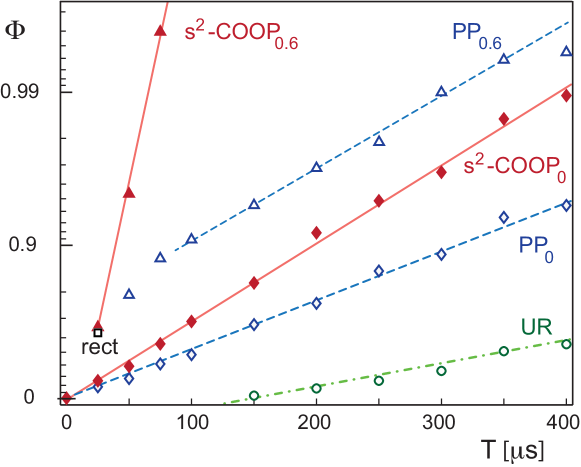
Figure 8: The figure shows the scaling of the performance $\Phi$ (cf. Eq. (35)) for different families of Ramsey sequences as a function of pulse duration $T$ for a bandwidth that is 7 times larger than the maximum pulse amplitude.

The analysis presented in the previous sections allowed us to clearly organize the large number of possible Ramsey sequence constructions in terms of pulse type (UR, PP_R, ST_R, s²-COOP_R) and the symmetry relation between the two pulses. From UR via PP_R and ST_R to s²-COOP_R pulses, the constraints for the individual pulses are more and more relaxed, i.e. the number of available degrees of freedom (represented by filled circles in Table 3) increases. The extent to which this translates in improved performance of Ramsey-type pulse sequences will be investigated in the following. In fact, striking differences in performance are found for the different pulse sequence families. The key results are summarized in Figure 8, which shows the achievable broadband quality factor $\Phi$ (cf. Eq. (35)) as a function of pulse duration $T$. The extracted parameters of interest are summarized in Table 4.

In previous systematic studies of broadband UR [20], PP₀ [13] and PP_R [40] pulses, it was empirically found that the performance $\Phi_{P}$ of a given pulse type scales with pulse duration $T$ roughly as

$$\Phi(T)\approx 1-c\ e^{-aT}$$ (65)

with constants $a$ and $c$. Hence, plotting $\tilde{\Phi}(T)=-{\rm ln}\{1-\Phi(T)\}$ as a function of $T$ is expected to approximately follow a straight line with slope $a$ and $y$-axis intercept $b=-{\rm ln}\{c\}$, which is indeed the case (cf. Fig. 8 and Table 4).

Fig. 9 shows the desired Ramsey fringe pattern given by Eq. (1) (grey curve) for an effective evolution period of $\tau_{eff}=\tau+\delta$ of 95 $\mu$s and the actual modulation of the $z$-component of the final Bloch vector $M^{\it final}_{z}(\nu)$ that can be achieved for a pulse duration of 75 $\mu$s by different pulse families (Fig. 9 A, B, D, E, F) and by a rectangular $90^{\circ}$ pulse (Fig. 9 C) with the same maximum pulse amplitude of 10 kHz and a corresponding pulse duration of 25 $\mu$s.

Figure 9: The grey and black curves show the desired ideal Ramsey fringe pattern and the simulated modulation of $M_{z}(\nu)$ for s²-COOP_0.6 (A) and PP_0.6 pulses (B), for rectangular 90^∘ pulses (C), for s²-COOP₀ (D), PP₀ (E) and UR pulses (F) (cf. Table 4) with a duration of $T=75\ \mu$s (except for the rectangular pulses with $T=25\ \mu$s). The effective evolution time $t_{\it eff}$ is 95 $\mu$s.

Broadband UR pulses: For the desired range of offsets and scaling factors of the pulse amplitude, individual UR(90${}_{y}^{\circ}$) pulses were optimized using the GRAPE algorithm as described in [15, 20]. The maximum performance $\Phi(T)$ of $S$-$\tau$-$S^{\prime}$ Ramsey sequences, where $S$ is a UR($90^{\circ}_{y}$) pulse and $S^{\prime}=S^{tr}_{ip}$ is indicated in Fig. 8 by open circles. Even for the longest considered pulse duration of $T$=400 $\mu$s, the quality factor is poor. As shown in Fig. 9 F, for the best Ramsey constructions based on UR pulses with a duration of 75 $\mu$s, the black curve representing $M^{\it final}_{z}(\nu)$ deviates strongly from the desired Ramsey fringe pattern (grey curve) over the entire offset range of interest.

Broadband PP₀ pulses: For the same pulse durations, a significantly improved performance is found for $S$-$\tau$-$S^{\prime}$ Ramsey sequences, where $S$ is a PP₀($z\to x$) pulse and $S^{\prime}=S^{tr}_{ip}$ as shown in Fig. 8 by open diamonds. The PP₀ pulses were optimized using the GRAPE algorithm described in [15, 46]. Note that PP₀ pulses with a duration of 75 $\mu$s achieve better quality factors than four times longer UR pulses. However, as illustrated in Fig. 9 E, $M^{\it final}_{z}(\nu)$ still deviated significantly from the desired fringe pattern. Fig. 10 D shows the detailed offset-dependent orientation of the Bloch vectors after the first Ramsey pulse (before the SQF filter) and Figs. 10 D^′ and 10 D^′′ shows the Bloch vectors after the second Ramsey pulse without and with ZQF filter, respectively.

Broadband s²-COOP₀ pulses: As shown by the filled diamonds in Fig. 8, a significant further improvement of pulse sequence performance is found for s²-COOP₀ pulses and identical pulse durations $T^{(1)}=T^{(2)}=T$ that were optimized using the algorithm outlined in section 4.2.2. In particular the slope $a$(s²-COOP${}_{0})\approx 12$ ms^-1 is larger compared to $a$(PP${}_{0})\approx 7.3$ ms^-1 and $a$(UR)$\approx 3.5$ ms^-1 (cf. Table 4). Although for short durations the absolute gains are moderate, this leads to markedly improved sequences for longer pulses that are required to reach reasonabaly good quality factors.

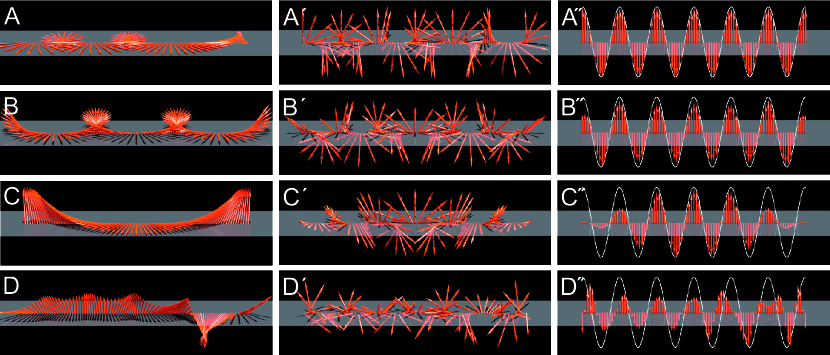
Figure 10: Panels A-D show the orientation of the Bloch vectors after the first Ramsey pulse before the SQF filter is applied for the pulses shown in Fig. 6 A-D, repectively: (A) s²-COOP_R pulses with $R=0.53$, (B) PP_R pulses with $R=0.53$, (C) rectangular 90^∘ pulses and (D) PP₀ pulses. The range of offsets is $-35$ kHz $\leq\nu\leq$ 35 kHz. The corresponding Bloch vectors after the second Ramsey pulse without (A^′-D^′) and with (A^′′-D^′′) ZQF filter are shown in the middle and right panels, respectively. The effective evolution time $t_{\it eff}$ is 85 $\mu$s and the dashed curves in the right panels represents the target Ramsey fringe pattern.

As the relative slope $R$ of s²-COOP₀ pulses is zero by definition, the auxiliary delay $\delta$ is also zero and the effective evolution time $t_{\it eff}$ of the Ramsey sequence is identical to the inter-pulse delay $\tau$ (as for UR and PP₀ pulses). The shapes of the pulse components $u_{x}(t)$ and $u_{y}(t)$ for s²-COOP₀ pulses with a duration of 75 $\mu$s are displayed in Figs. 6 D.

Rectangular pulses: At first sight, it may be surprising that the quality factor $\Phi=0.62$ of a Ramsey sequence based on simple rectangular pulses (indicated by an open square in Fig. 8) is markedly better than the performance based on highly optimized s²-COOP₀ pulses of comparable duration. However, this is a simple result of the fact that in contrast to UR, PP₀ and s²-COOP₀ pulses, which yield Ramsey sequences with a vanishing auxiliary delay ($\delta=0$), $\delta$ is not zero for rectangular 90^∘ pulses. This ensues from the non-vanishing linear part of $\alpha(\omega)$ of rectangular 90^∘ pulses [56] with a relative slope of $R^{\it rect}_{\alpha}\approx 0.64$, cf. Eq. (63). This is illustrated in Fig. 6 C, where the effective evolution time $t_{\it eff}=85$ $\mu$s consists of an inter-pulse delay $\tau=53$ $\mu$s and the effective auxiliary delay $\delta=2\cdot R^{\it rect}_{\alpha}\cdot 25$ $\mu$s=32 $\mu$s. The offset-dependent positions of the Bloch vectors after the first rectangular pulse are shown in Fig. 10 C. Note that for offsets $|\nu|>u^{max}$=10 kHz, the Bloch vectors still have significant $z$-components (that will be eliminated by the following SQF filter) because the Euler angle $\beta(\omega)$ does deviate considerably from the desired value of $90^{\circ}$ for these offsets. Figs. 10 C^′ and C^′′ show the orientation of the Bloch vectors after the second rectangular pulse without and with zero-quantum filter, respectively. For $t_{\it eff}=95$ $\mu$s, the resulting modulation of its $z$-component is also represented by the black curve in Fig. 9 C. As expected, the desired ideal fringe pattern indicated by the grey curve is closely matched for small offsets $|\nu|$, but cannot be approached if $|\nu|$ is larger than $u^{max}$. As pointed out in section 2.1, for many applications the non-vanishing auxiliary constant delay $\delta$ of rectangular pulses is acceptable and it is particularly interesting to see the impact on the performance of Ramsey sequences if the condition $R=0$ (and hence $\delta=0$) is lifted for PP_R, ST_R and s²-COOP_R pulses.

Broadband PP_R pulses: The open circles in Fig. 5 show the Ramsey quality factor $\Phi$ of PP_R pulses $S$ (and $S^{\prime}=S^{tr}_{ip}$) of duration $T=75$ $\mu$s that were optimized for different slopes $R$ based on the GRAPE-based approach described in [40]. Their performance is significantly better than the quality factor $\Phi$ that is reached by rectangular pulses, which is marked in Fig. 5 by an open rectangle. The best performance of the PP_R pulses ($\Phi=0.88$) is found for $R=0.6$. The pulse shape for $R=0.53$ (with $\Phi=0.87$) is shown in Fig. 6 B. The pulse has a vanishing $x$-component ($u_{x}(t)=0$) and the $y$-component $u_{y}(t)$ alternates between the values $\pm u^{\it max}$. The effective evolution time $t_{\it eff}=85$ $\mu$s consists of an inter-pulse delay $\tau=5.5$ $\mu$s and the effective evolution time during the pulses is $\delta=2R\cdot 75\mu$s=79.5$\mu$s. The offset-dependent orientation of the Bloch vectors after the first and the second pulse are shown in Fig. 10 B and B^′ (and in B^′′ after the ZQF). Figs. 9 B and 10 B^′′ demonstrate that the desired fringe pattern is approached for the entire offset range of interest. Compared to the case of rectangular pulses, the overall deviation from the ideal pattern are smaller and evenly distributed over the entire offset range, because the gradients for all offsets were given the same weight in the optimization of the PP_R pulses. As the best value of $R$ for PP_R pulses with a duration of $T=75$ $\mu$s was 0.6, PP_0.6 pulses were also optimized for other pulse durations $T$ and the resulting Ramsey sequence quality factors $\Phi$ are shown by open triangles in Fig. 8.

Table 4: Comparison of the auxiliary delay $\delta$ and scaling parameters of quality factor $\Phi(T)$ for the Ramsey pulse families shown in Fig. 8.

$S^{(1)}$	$S^{(2)}$	$\delta$ [$\mu$s]	$a$ [ms-1]	$b$	c	$\Phi(T=75$ $\mu$s)	$T_{\Phi=0.996}$ [$\mu$s]
$S^{(1)}_{\rm COOP_{0.6}}$	$S^{(2)}_{\rm COOP_{0.6}}$	90	90	-1.3	3.7	0.996	75
ST0.6	$S^{tr}_{ps}$	90	90	-1.3	3.7	0.996	75
PP0.6	$S^{ip}_{ip}$	90	11	1.3	0.27	0.88	$\approx$400
$S^{(1)}_{\rm COOP_{0}}$	$S^{(2)}_{\rm COOP_{0}}$	0	12	0	1	0.56	$\approx$460
ST0	$S^{tr}_{ps}$	0	12	0	1	0.56	$\approx$460
PP0	$S^{ip}_{ip}$	0	7.3	0	1	0.4	$\approx$750
UR	$S^{ip}_{ip}$	0	3.5	-0.5	1.65	$<0$	$\approx$1700

The auxiliary delay $\delta$ corresponds to a pulse duration $T=75$ $\mu$s. For each pulse type, the slope $a$

and axis intercept $b$ are determined from Fig. 8 and $c=e^{-b}$. With these parameters, the quality

factor scales with $T$ approximately as $\Phi\approx 1-e^{-aT-b}=1-c\ e^{-aT}$.

Broadband ST_R and s²-COOP_R pulses As discussed in section 5 for the pulse duration $T=75$ $\mu$s the best quality factor of $\Phi=0.9965$ is achieved for $R=0.53$. However, as rectangular pulses and the best PP_R pulses have values of $R\approx 0.6$, we also chose this value (corresponding to $\Phi=0.9960$) for the comparison of the performance as a function of pulse duration $T$ in Fig. 8. This figure illustrates the far superior performance that can be achieved by s²-COOP_R pulses compared to rectangular pulses, PP_R pulse and UR pulses.

Fig. 10 A shows that the first pulse brings the Bloch vectors almost completely into the transverse plane for all offset frequencies. This figure also illustrates the nonlinear phase roll, which provides significantly more flexibility in the pulse optimization. Although the offset-dependent orientations of the Bloch vectors after the second pulse appear to be rather chaotic (cf. Fig. 10 A^′), their $z$-components do approach the desired Ransey fringe pattern with outstanding fidelity (cf. Fig. 10 A^′′). In fact, in Fig. 9 A, $M^{\it final}_{z}(\nu)$ and the ideal Ramsey fringe pattern are indistinguishable due to the excellent match.

The s²-COOP_R pulse shapes for $R=0.53$ are displayed in Fig. 6 A. As discussed in sections 5 and 6.2, the s²-COOP_R pulse pair corresponds to a very good approximation to pairs of ST_R pulses with $S^{\prime}=S^{\it tr}_{\it ps}$. In fact, for the optimization parameters considered here, the performance of s²-COOP_R Ramsey pulses is closely approached by the family of ST_R pulses.

Fig. 8 demonstrates that the excellent quality factor $\Phi$ of s²-COOP_R and ST_R pulses not only exceed by far the performance of simple rectangular pulses but also results in ultra short pulses compared to conventional approaches based on individually optimized pulses. The line fitting the data in Fig. 8 corresponds to an extremely steep slope of $a$(s²-COOP${}_{0.6})\approx 90$ ms^-1 (and $y$-axis intercept $b$(s²-COOP${}_{0.6})\approx-1.3$). Note that a Ramsey quality factor $\Phi>0.996$ can be achieved by s²-COOP_R and ST_R pulses with a duration $T=75$ $\mu$s, which is only three times longer than the duration of a rectangular 90^∘ pulse. For comparison, based on a simple extrapolation of the data shown in Fig. 8, a comparable quality factor is expected to require durations in the order of $T\approx 400$ $\mu$s for PP_R pulses, $T\approx 750$ $\mu$s for PP₀ pulses, and about 1.7 ms for UR pulses, corresponding to 16, 30 and more than 70 times the duration of a rectangular 90^∘ pulse, respectively.

8 Experimental demonstration

As pointed out in section 1.1, the Ramsey sequence plays an important role in many fields, including 2D NMR spectroscopy, where it is used as a standard frequency-labeling building block in many experiments [1]. The specific parameters (maximum pulse amplitude, desired bandwidth of frequency offsets, etc.) of the optimization problem defined in section 5 were motivated by applications of 2D nuclear Overhauser enhancement spectroscopy (NOESY), where the bandwidth of interest is much larger than the maximum available pulse amplitude. More specifically, it was assumed that the desired bandwidth is seven times larger than the maximum control amplitude of 10 kHz, corresponding e.g. to ¹³C-¹³C-NOESY experiments at high magnetic fields.

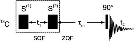
Figure 11: Schematic representation of the 2D-¹³C-¹³C-NOESY pulse sequence [36] that was used to demonstrate the performance of different types of Ramsey pulses $S^{(1)}$ and $S^{(2)}$ which form the frequency labeling element of the NOESY experiment indicated by the dashed rectangle. ¹H spins were decoupled using the composite-pulse sequence WALTZ-16 [43] (not shown).

To test the outstanding theoretical properties of s²-COOP sequences in practice, we performed 2D-¹³C-¹³C-NOESY experiments on a Bruker AV III 600 spectrometer with a magnetic field strength of 14 Tesla using a sample of ¹³C-labeled $\gamma$-D-glucose dissolved in Dimethylsulfoxid (DMSO). The ¹³C-¹³C-NOESY pulse sequence from [36] was used (without the ¹⁵N-decoupling pulses which were not necessary for the glucose test sample). The zero-quantum filter (ZQF) after the frequency labeling building block, i.e. after the second Ramsey pulse (cf. Fig. 11) was implemented by a standard chirp pulse/gradient pair [44]. The complete pulse sequence of the ¹³C-¹³C-NOESY experiment is shown schematically in Fig. 11, where the $S^{(1)}$-$\tau$-$S^{(2)}$ Ramsey-type frequency-labeling building block is indicated by the dashed box and the inter-pulse delay $\tau$ corresponds to the evolution period that is usually called "$t_{1}$" in 2D NMR.

In the experiments, the two 90^∘ pulses of the Ramsey building block were implemented by the following three pulse sequences: the s²-COOP_0.6 pulse pair with a duration $T=3/(4u^{max})$ (which is three times longer the duration of a rectangular 90^∘ pulse with the same maximum pulse amplitude $u^{max}$), the PP_0.6 pulse pair with the same pulse duration and as a pair of standard rectangular pulses.

The chemical shift range of 40 ppm for the ¹³C glucose sample at 14 Tesla corresponds to a bandwidth of about 6 kHz. As the Ramsey pulses were optimized for the challenging case of $\Delta\nu=7u^{max}$, a correspondingly scaled maximum pulse amplitude of $u^{max}=0.86$ kHz was used in the demonstration experiments. For this amplitude, the pulse durations $T$ were 870 $\mu$s for the s²-COOP_0.6 and PP_0.6 pulses and 290 $\mu$s for the rectangular pulses. In all experiments, the final detection pulse after the NOESY mixing period $\tau_{mix}$ was a strong rectangular 90^∘ pulse with a pulse amplitude of 12.2 kHz (and a corresponding duration of 20.5 $\mu$s), which was sufficient to cover the bandwidth of 6 kHz. For larger bandwidths, this pulse could be replaced by an optimized broadband excitation pulse [13].

The NOESY mixing time was $\tau_{mix}=50$ ms and the recycle delay between scans was 280 ms. The spectra were recorded at a temperature of 293 K, using a TXI probe with 512 $t_{1}$ increments, 16 scans for each increment and 8k data points in the detection period $t_{2}$. As the minimum $t_{1}$ value is given by $\delta=2RT=2\cdot 0.6\cdot 870$ $\mu$s$\ =\$1.04 ms (cf. Eq. (37)), the time-domain data was completed using standard backward linear prediction [57] before the 2D Fourier transform. The processing parameters for all spectra were identical. Selected slices of the ¹³C-¹³C NOESY spectra for s²-COOP_0.6, PP_0.6 and conventional rectangular pulses are displayed in Fig. 12 A-C.

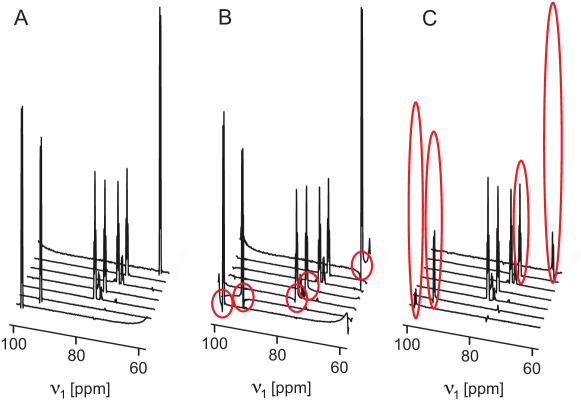
Figure 12: The figure shows cross sections of 2D-¹³C-¹³C-NOESY experiments of ¹³C-labeled $\gamma$-D-glucose. The pulses $S^{(1)}$ and $S^{(2)}$ of the Ramsey-type frequency-labeling block indicated by the dashed box in Fig. 11 were s²-COOP_0.6 pulses (A), PP_0.6 pulses (B) and rectangular 90^∘ pulses (C). In B, the ellipses indicate signal distorsions due to phase errors. In C, the ellipses point out amplitude losses relative to A.

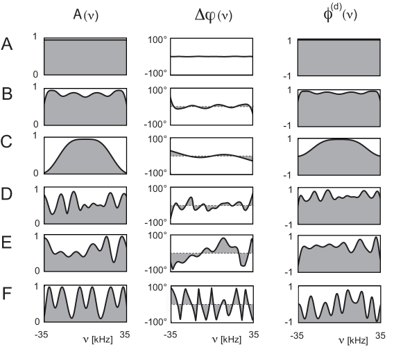
Figure 13: The simulated signal amplitude $A(\nu)$ (left column) and phase error $\Delta\varphi(\nu)$ in the $\nu_{1}$ dimension (middle column) of a 2D-NOESY spectrum is shown as a function of offset frequency $\nu$ for s²-COOP_0.6 pulses (A), PP_0.6 pulses (B), rectangular 90^∘ pulses (C), s²-COOP₀ pulses (D), PP₀ pulses (E) and UR pulses (F). The right column shows the offset-dependent Ramsey quality factor $\phi^{(d)}(\nu)$, which reflects both pulse amplitude and phase errors.

As expected from the simulations shown in Fig. 9 C, rectangular pulses perform well for relatively small offsets frequencies (corresponding to the center of the spectra in Fig. 12, i.e. to the signals in the chemical shift range from 70 to 80 ppm). However, for large offsets from the irradiation frequency at the center of the spectrum, the performance of rectangular pulses breaks down (cf. Fig. 9 C), resulting in a dramatic signal loss for the peaks in the NOESY experiments that are located at the edge of the spectral range (near 60 ppm and 100 ppm) in Fig. 12 C. In contrast, s²-COOP_0.6 pulses also perform perfectly well for large offsets (cf. Fig. 9 C), resulting in large gains of up to an order of magnitude for the signal amplitudes at the edge of the spectral range. As expected from the simulated fringe patterns in Fig. 9 B, PP_0.6 pulses also yield significantly increased signal amplitudes for large offset frequencies compared to rectangular pulses. However, as shown in Fig. 12 B, the peaks also have relatively large phase errors, resulting in asymmetric line-shapes and baseline distortions close to large peaks (indicated by the ellipses). The corresponding simulated offset dependence of the signal amplitude $A(\nu)$ and of the phase error $\Delta\varphi(\nu)$ in the $\nu_{1}$ dimension (corresponding to the evolution period $t_{1}$ in the time domain) can be calculated based on the Euler angles $\beta^{(1)}$ and $\beta^{(2)}$ and the nonlinear components of $\alpha^{(1)}$ and $\gamma^{(2)}$ as

$$A(\nu)=\sin\{\beta^{(1)}(\nu)\}\sin\{\beta^{(2)}(\nu)\}\ \ \ {\rm and}\ \ \ \Delta\varphi(\nu)=\alpha^{(1)nl}(\nu)+\gamma^{(2)nl}(\nu)$$ (66)

(cf. Eq. (15)) and are shown in the left and middle panels of Fig. 13 A-F, respectively. The quality factor $\Phi^{(d)}(\nu)$ defined in Eq. (31) can also be expressed in terms of $A(\nu)$ and $\Delta\varphi(\nu)$ as

$$\Phi^{(d)}(\nu)=A(\nu)\cos\{\Delta\varphi(\nu)\},$$ (67)

i.e. it reflects both $A(\nu)$ and $\Delta\varphi(\nu)$ as shown in panels of Fig. 13 A-F. We note in passing that for applications with specific weights $w_{A}$ and $w_{\Delta\varphi}$ for amplitude and phase errors, a tailor-made quality factor

$$\Phi^{e}(\nu)=1-w_{A}\{1-A(\nu)\}^{2}-w_{\Delta\varphi}\{\Delta\varphi(\nu)\}^{2}$$ (68)

could be used in the optimizations.

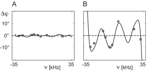
Figure 14: Expanded view of the simulated phase errors shown in Fig. 13 A and B for s²-COOP_0.6 pulses and PP_0.6 pulses, respectively (black curves). Experimentally measured phase errors $\Delta\varphi(\nu)$ based on the spectra displayed in Figs. 12 A and B are shown by open squares.

Whereas the s²-COOP_0.6 pulses create almost ideal signal amplitudes $A(\nu)\approx 1$ (cf. left panel of Fig. 13 A) for all frequencies $\nu$ in the optimized offset range, for the PP_0.6 pulses the signal amplitude varies between 0.7 and 0.9 (cf. left panel of Fig. 13 B). Similarly, the phase errors $\Delta\phi(\nu)$ are smaller than 1.5^∘ for the s²-COOP_0.6 pulses (cf. middle panel of Fig. 13 A), whereas noticeable phase errors of more than $\pm 10^{\circ}$ are created by the PP_0.6 pulses (cf. middle panel of Fig. 13 B). Panels A and B in Fig. 14 show enlarged views of these phase errors. In addition to the simulated curves, Fig. 14 also shows experimentally determined phase errors (open squares) based on the spectra displayed in Figs. 12 A and B. A reasonable match is found between experimental and simulated data, confirming the superior performance of s²-COOP_R pulses compared to conventional PP_R and rectangular pulses in broadband Ramsey-type pulse sequences. The pulses with $\delta=0$ (corresponding to $R=0$) have significantly poorer performance both in terms of signal amplitude and phase for the same pulse durations, as shown in Fig. 13 D-F.

9 Conclusions and outlook

Here, we introduced the concept of s²-COOP pulses that are optimized simultaneously and act in a cooperative way in the same scan. Pulse cooperativity within the same scan (cf. Fig. 1 A) complements the multi-scan COOP approach introduced in [28] (cf. Fig. 1 B). A general filter-based approach was introduced in section 4.1 that makes it possible to simultaneously optimize an arbitrary number of s²-COOP pulses. This makes it possible to optimize entire pulse sequences, rather than isolated pulses. The proposed s²-COOP quality factors are based on the desired transfer function of the pulse sequence, which is essentially a product of the transfer functions of the individual pulses and filter elements. This is in contrast to the tracking approach for the optimization of decoupling sequences [67, 68, 69], where the overall performance of a multiple-pulse sequence depends on the sum of the deviations from the ideal transfer function during the pulse sequence.

As an illustrative example of s²-COOP pulses, we analyzed the important class of Ramsey-type experiments. Based on this analysis, a symmetry-adapted approach for the optimization of s²-COOP pulse pairs for Ramsey sequences was discussed in section 4.2 that provides a different perspective and additional insight into this optimization problem. However, it is limited to the optimization of two pulses, in contrast to the general filter-based approach discussed in section 4.1, which does not have this limitation. The development of s²-COOP Ramsey sequences provides excellent ultra short broadband pulses with a bandwidth that can be much larger than the maximum available pulse amplitude. In the chosen example, the bandwidth was seven times larger than the pulse amplitude, but the proposed algorithms can of course also be applied to even larger bandwidths. Compared to conventional approaches based on the isolated optimization of individual pulses such as universal rotation (UR) pulses [20], point-to point pulses with constant phase of the final magnetization as a function of offset (called PP₀ pulses) and pulses that create a linear phase slope as a function of offset (called PP_R pulses or Iceberg pulses [40]), the minimum pulse duration to reach the required overall performance of a Ramsey experiment is up to two orders of magnitude shorter for s²-COOP. Decreased pulse durations result in reduced relaxation losses during the pulses, less experimental imperfections and also less sample heating, which is particularly important for in vivo spectroscopy and applications in medical imaging. The analysis of the resulting Ramsey s²-COOP pulses also lead to the discovery of the powerful class of ST_R pulses discussed in section 6, which makes it possible to construct Ramsey sequences based on the individual optimization of pulses, closely approaching the performance of s²-COOP pulses for the optimization parameters considered here.

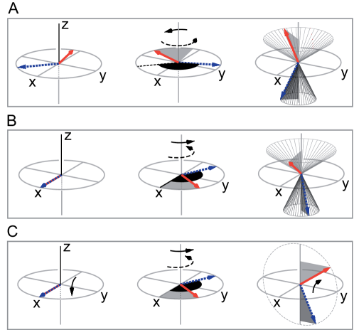
Figure 15: Graphical representation of the orientation of two exemplary Bloch vectors with different offset frequencies $\omega$ after the first Ramsey pulse (left), after the inter-pulse delay $\tau$ (middle) and after the second Ramsey pulse (right) for the same effective evolution time $t_{\it eff}$. Panel A corresponds to the case of s²-COOP_R and PP_R pulses with $R\neq 0$ and to s²-COOP₀, where the vectors are not necessarily oriented along the $x$-axis after the first pulse. Panel B corresponds to the case of PP₀ pulses and panel C corresponds to the case of UR pulses and ideal hard pulses.

When comparing Ramsey pulses with the same duration $T$, the significant performance gain from UR via PP_R to ST_R and s²-COOP_R pulses demonstrated in Figs. 8, 9 and 13 is strongly correlated with the increasing number of degrees of freedom (cf. Table 3) for the offset-dependent Euler angles of these pulse types.

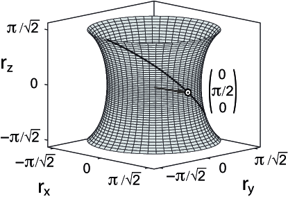
Figure 16: The figure shows the allowed effective rotation vectors ${\bf r}$ for different types of Ramsey pulses $S^{1}$, where the length of ${\bf r}$ is given by the rotation angle (in units of radians) and its orientation corresponds to the rotation axis. The arrow represents a rotation by $90^{\circ}$ around the $y$-axis, corresponding to UR pulses and ideal hard pulses. In the case of PP₀ pulses, the Bloch vectors are also brought from $z$ to $x$ (Fig. 15 B), but the rotation axis is not fixed to the $y$-axis [20, 49]. The black curve illustrates the locations of the tips of the allowed effective rotation vectors of PP₀ pulses. For PP_R, ST_R and s²-COOP_R pulses, the effective rotation vectors of the individual Ramsey pulses can be located anywhere on the grey surface [49, 58].

It is also instructive to consider the increasing flexibility in terms of the effective rotation vectors of the individual pulses and the trajectories of Bloch vectors during the Ramsey sequence. Fig. 15 schematically displays the orientations of two exemplary Bloch vectors with different offset frequencies $\omega$ after the first Ramsey pulse (left), after the inter-pulse delay $\tau$ (middle) and after the second Ramsey pulse (right). For ideal UR pulses, which are most restrictive, the effect of the first pulse is a $90^{\circ}$ rotation around the $y$-axis, bringing both initial Bloch vectors from the $z$-axis to the $x$-axis (Fig. 15 C). The corresponding rotation vector ${\bf r}$ of the UR($90^{\circ}_{y}$) pulse with components $r_{x}=0$, $r_{y}=\pi/2$ and $r_{z}=0$ is represented in Fig. 16 by an arrow and the location of its tip is indicated by a circle. In the case of PP₀ pulses, the Bloch vectors are also brought from $z$ to $x$ (Fig. 15 B), but the rotation axis is not fixed to the $y$-axis [49, 20]. For example, a rotation by 180^∘ around the axis ${1\over{\sqrt{2}}}({\bf e}_{x}+{\bf e}_{z})$ (corresponding to the bisecting line of the angle between the $x$ and $z$-axis) has the same result and the black curve in Fig. 16 indicates the set of all rotation vectors that are compatible with a PP₀($z\rightarrow x$) pulse. In the case of PP_R, ST_R and s²-COOP_R pulses, the first pulse is allowed to bring the Bloch vectors from the north pole (i.e. from the $z$-axis) to different locations on the equator of the Bloch sphere (cf. Fig. 15 A). Hence, the allowed rotation vectors are not limited to the black curve in Fig. 16, but can be located anywhere on the grey surface [49, 58]. Whereas for PP_R pulses the angles between the $x$-axis and the Bloch vector on the equator (i.e. the phase of the Bloch vector, which is identical to the Euler angle $\alpha(\omega)$) is required to be a linear function of the offset frequency (cf. Table 3), this condition is lifted for ST_R and s²-COOP_R pulses. As illustrated in Fig. 15, the two Bloch vectors rotate during the delay $\tau$ by different angles $\omega\tau$ around the $z$-axis. In the most restricted case of UR pulses, the following UR($90^{\circ}_{-y}$) pulse brings all Bloch vectors from the equator into the $y$-$z$-plane (cf. Fig. 15 C). In contrast, the final Bloch vectors for PP₀ (Fig. 15 B) and PP_R, ST_R and s²-COOP_R pulses (Fig. 15 C) are not required to be located in this plane. However, the conditions for the Euler angles summarized in Table 3 ensure that for each offset frequency $\omega$, the $z$-component of the final Bloch vector corresponds to the value defined by the target fringe pattern of Eq. (1). Hence for these pulse types, for each offset the final Bloch vector is only required to be located on a cone around the $z$-axis. In Fig. 15, the projections of the Bloch vectors onto the $z$-axis are indicated by grey triangles.

The presented optimal-control based approach for the efficient optimization of s²-COOP pulses can be generalized in a straightforward way to take into account additional aspects of practical interest such as restrictions on the power or total energy of the control pulses (cf. [19]), effects of amplitude and phase transients [50] or the effects of relaxation during the pulses [59]. In systematic studies of broadband UR [20], PP₀ [13] and PP_R [40] pulses, it was found that for a desired value of the quality factor, the minimum pulse duration $T$ scales roughly linearly with the bandwidth $\Delta\nu$ and a similar scaling behavior is expected for s²-COOP_R pulses.

In addition to standard Ramsey experiments and e.g. the precise measurement of magnetic fields for a large range of field amplitudes [60], potential applications of ST_R and s²-COOP_R Ramsey pulses include stimulated echoes as well as two-dimensional spectroscopy. The specific optimization parameters of the challenging test case considered here was motivated by 2D-¹³C-¹³C-NOESY experiments at future spectrometers with ultra-high magnetic field strengths that are currently under development. However, the presented algorithms can of course be used to optimize the performance of Ramsey-type pulse sequence elements for any desired set of experimental parameters. For example, significant gains compared to conventional approaches are already expected if s²-COOP pulses are designed for bandwidths corresponding to currently available field strengths. In addition to the frequency labeling blocks of 2D-NOESY experiments discussed here, in NMR spectroscopy the novel Ramsey 90^∘-$\tau$-90^∘ building blocks can be directly applied in many other 2D experiments, such as 2D exchange spectroscopy [1, 34] and also in heteronuclear correlation experiments such as heteronuclear single quantum coherence spectroscopy (HSQC) [61] and heteronuclear multiple quantum coherence spectroscopy (HMQC) [62]. For example, s²-COOP Ramsey pulses can be used as initial and final pulses in a modified INEPT block [63], where instead of the standard central 180^∘ refocusing pulses two inversion pulses are applied to the spins of both nuclei [64, 65, 66], provided that the phase of the second Ramsey pulse is shifted by 90^∘.

Beyond the Ramsey scheme, which was considered here merely as an illustrative example, it is expected that s²-COOP pulses will find numerous applications in the control of complex quantum systems in spectroscopy, imaging and quantum information processing. In particular, the presented approach for the optimization of s²-COOP pulses can be used for the efficient and robust control schemes of general quantum systems and is not limited to the control of spin systems.

10 Appendix

10.1 Derivation of the relations between the Euler angles of $S$ and $S^{\prime}$

In Table 1, the relations between the offset-dependent Euler angles of pulses $S$ and $S^{\prime}\in\{S^{-1},\ S_{ps},\ S_{ip},\ S^{tr},\ S^{tr}_{ps},S^{tr}_{ip}\}$ were summarized. Here it is shown explicitly how these relations can be derived from well known properties of rotation operators [38, 10, 49, 20].

For a given pulse $S$, the corresponding offset-dependent rotation operator ${\bf S}(\omega)$ can be expressed in the ZYZ convention [38] in terms of the offset-dependent Euler angles $\gamma(\omega)$, $\beta(\omega)$ and $\alpha(\omega)$ as

$${\bf S}(\omega)={\bf R}_{z}\{\alpha(\omega)\}{\bf R}_{y}\{\beta(\omega)\}{\bf R}_{z}\{\gamma(\omega)\},$$ (69)

i.e. as a sequence of rotation operators ${\bf R}_{a}\{\varphi\}$ with rotation axis $a$ and rotation angle $\varphi$. As usual, the rotations operators are ordered from right to left, i.e. in Eq. (69) ${\bf R}_{z}\{\gamma(\omega)\}$ is applied first, followed by ${\bf R}_{y}\{\beta(\omega)\}$ and ${\bf R}_{z}\{\alpha(\omega)\}$.

10.2 $S^{\prime}=S^{-1}$

$${\bf S}^{-1}(\omega) = \big{(}{\bf R}_{z}\{\alpha(\omega)\}\ {\bf R}_{y}\{\beta(\omega)\}\ {\bf R}_{z}\{\gamma(\omega)\}\big{)}^{-1}$$ (70)

$$= {\bf R}^{-1}_{z}\{\gamma(\omega)\}\ {\bf R}^{-1}_{y}\{\beta(\omega)\}\ {\bf R}^{-1}_{z}\{\alpha(\omega)\}$$

$$= {\bf R}_{z}\{-\gamma(\omega)\}\ {\bf R}_{y}\{-\beta(\omega)\}\ {\bf R}_{z}\{-\alpha(\omega)\}.$$

In the second line we used the standard relation $(ABC)^{-1}=C^{-1}B^{-1}A^{-1}$ and in the third line we used the fact that the inverse of a rotation operator is simply obtained by inverting the sign of the rotation angle.

10.3 $S^{\prime}=S_{ps}$

According to Table 1, for $S^{\prime}=S_{ps}$ the pulse amplitude $u_{ps}(t)$ and pulse phase $\xi_{ps}(t)$ is given by

$$u_{ps}(t)=u(t),\ \ \ {\rm and}\ \ \ \xi_{ps}(t)=\xi(t+\pi).$$ (71)

This corresponds to a $180^{\circ}$ rotation of the overall rotation operator ${\bf S}(\omega)$ around the $z$ axis:

$${\bf S}_{ps}(\omega) = {\bf R}_{z}\{\pi\}{\bf S}(\omega){\bf R}^{-1}_{z}\{\pi\}.$$ (72)

Inserting Eq. (69) in Eq. (72), we find

$${\bf S}_{ps}(\omega) = {\bf R}_{z}\{\pi\}\ {\color[rgb]{0,0,1}{\bf R}_{z}\{\alpha(\omega)\}{\bf R}_{y}\{\beta(\omega)\}{\bf R}_{z}\{\gamma(\omega)\}}\ {\bf R}^{-1}_{z}\{\pi\}$$ (73)

$$= {\color[rgb]{0,0,1}{\bf R}_{z}\{\alpha(\omega)\}}\ {\bf R}_{z}\{\pi\}{\color[rgb]{0,0,1}{\bf R}_{y}\{\beta(\omega)\}}{\bf R}^{-1}_{z}\{\pi\}\ {\color[rgb]{0,0,1}{\bf R}_{z}\{\gamma(\omega)\}}$$

$$= {\bf R}_{z}\{\alpha(\omega)\}\ {\color[rgb]{0,0,1}\big{(}{\bf R}_{z}\{\pi\}{\bf R}_{y}\{\beta(\omega)\}{\bf R}^{-1}_{z}\{\pi\}\big{)}}\ {\bf R}_{z}\{\gamma(\omega)\}$$

$$= {\bf R}_{z}\{\alpha(\omega)\}\ {\color[rgb]{0,0,1}{\bf R}_{y}\{-\beta(\omega)\}}\ {\bf R}_{z}\{\gamma(\omega)\},$$

where the color is used to emphasize the individual transformations in each line. In the second line we used the fact that rotations around the same axis commute and in the third line the terms are simply recolored to emphasize the relevant grouping for the next transformation. The well known relation

$${\bf R}_{a}\{\pi\}{\bf R}_{b}\{\varphi\}{\bf R}^{-1}_{a}\{\pi\}={\bf R}_{-b}\{\varphi\}={\bf R}_{b}\{-\varphi\},$$ (74)

which holds for arbitrary orthogonal rotation axes $a$ and $b$ and arbitrary angles $\varphi$ [49, 20], was used in the fourth line with $a=z$, $b=y$ and $\varphi=\beta(\omega)$.

10.4 $S^{\prime}=S_{ip}$

According to Table 1, for $S^{\prime}=S_{ip}$ the pulse amplitude $u_{ip}(t)$ and phase $\xi_{ip}(t)$ is given by

$$u_{ip}(t)=u(t),\ \ \ {\rm and}\ \ \ \xi_{ip}(t)=-\xi(t).$$ (75)

As shown in [10, 49], ${\bf S}_{ip}(\omega)$ is related to ${\bf S}(-\omega)$ via

$${\bf S}_{ip}(\omega) = {\bf R}_{x}\{\pi\}{\bf S}(-\omega){\bf R}^{-1}_{x}\{\pi\}.$$ (76)

Replacing $\omega$ by $-\omega$ in Eq. (69), ${\bf S}_{ip}(\omega)$ can be expressed in the form

$${\bf S}_{ip}(\omega) = {\bf R}_{x}\{\pi\}\ \ {\color[rgb]{0,0,1}{\bf R}_{z}\{\alpha(-\omega)\}{\bf R}_{y}\{\beta(-\omega)\}{\bf R}_{z}\{\gamma(-\omega)\}}\ \ {\bf R}^{-1}_{x}\{\pi\}$$ (77)

$$= {\bf R}_{x}\{\pi\}{\bf R}_{z}\{\alpha(-\omega)\}\ \ {\color[rgb]{0,0,1}{\bf R}^{-1}_{x}\{\pi\}{\bf R}_{x}\{\pi\}}\ \ {\bf R}_{y}\{\beta(-\omega)\}{\bf R}_{z}\{\gamma(-\omega)\}{\bf R}^{-1}_{x}\{\pi\}$$

$$= {\color[rgb]{0,0,1}\big{(}{\bf R}_{x}\{\pi\}{\bf R}_{z}\{\alpha(-\omega)\}{\bf R}^{-1}_{x}\{\pi\}\big{)}}\ \ {\bf R}_{x}\{\pi\}{\bf R}_{y}\{\beta(-\omega)\}{\bf R}_{z}\{\gamma(-\omega)\}{\bf R}^{-1}_{x}\{\pi\}$$

$$= {\color[rgb]{0,0,1}{\bf R}_{z}\{-\alpha(-\omega)\}}\ \ {\bf R}_{x}\{\pi\}{\bf R}_{y}\{\beta(-\omega)\}{\bf R}_{z}\{\gamma(-\omega)\}{\bf R}^{-1}_{x}\{\pi\}$$

$$= {\bf R}_{z}\{-\alpha(-\omega)\}\ \ {\bf R}_{x}\{\pi\}{\bf R}_{y}\{\beta(-\omega)\}\ \ {\color[rgb]{0,0,1}{\bf R}^{-1}_{x}\{\pi\}{\bf R}_{x}\{\pi\}}\ \ {\bf R}_{z}\{\gamma(-\omega)\}{\bf R}^{-1}_{x}\{\pi\}$$

$$= {\bf R}_{z}\{-\alpha(-\omega)\}\ \ {\bf R}_{x}\{\pi\}{\bf R}_{y}\{\beta(-\omega)\}{\bf R}^{-1}_{x}\{\pi\}\ \ {\color[rgb]{0,0,1}\big{(}{\bf R}_{x}\{\pi\}{\bf R}_{z}\{\gamma(-\omega)\}{\bf R}^{-1}_{x}\{\pi\}\big{)}}$$

$$= {\bf R}_{z}\{-\alpha(-\omega)\}\ \ {\bf R}_{x}\{\pi\}{\bf R}_{y}\{\beta(-\omega)\}{\bf R}^{-1}_{x}\{\pi\}\ \ {\color[rgb]{0,0,1}{\bf R}_{z}\{-\gamma(-\omega)\}}$$

$$= {\bf R}_{z}\{-\alpha(-\omega)\}\ \ {\color[rgb]{0,0,1}\big{(}{\bf R}_{x}\{\pi\}{\bf R}_{y}\{\beta(-\omega)\}{\bf R}^{-1}_{x}\{\pi\}\big{)}}\ \ {\bf R}_{z}\{-\gamma(-\omega)\}$$

$$= {\bf R}_{z}\{-\alpha(-\omega)\}\ \ {\color[rgb]{0,0,1}{\bf R}_{y}\{-\beta(-\omega)\}}\ \ {\bf R}_{z}\{-\gamma(-\omega)\}.$$

In the second and fifth line, the identity operator ${\bf R}^{-1}_{x}\{\pi\}{\bf R}_{x}\{\pi\}={\bf 1}$ was inserted. Eq. (74) was used in line 4 with $a=x$, $b=z$, $\varphi=\alpha(-\omega)$, in line 7 with $a=x$, $b=z$, $\varphi=\gamma(-\omega)$ and in line 9 with $a=x$, $b=y$, $\varphi=\beta(-\omega)$.

10.5 $S^{\prime}=S^{tr}$

According to Table 1, for $S^{\prime}=S^{tr}$ the pulse amplitude $u^{tr}(t)$ and phase $\xi^{tr}(t)$ is given by

$$u^{tr}(t)=u(T-t),\ \ \ {\rm and}\ \ \ \xi^{tr}(t)=\xi(T-t).$$ (78)

As shown in [10, 49], ${\bf S}^{tr}(\omega)$ is related to ${\bf S}(-\omega)$ via

$${\bf S}^{tr}(\omega) = {\bf R}_{z}\{\pi\}{\bf S}^{-1}(-\omega){\bf R}^{-1}_{z}\{\pi\}.$$ (79)

Based on Eq. (70),

$${\bf S}^{-1}(-\omega) = {\bf R}_{z}\{-\gamma(-\omega)\}\ {\bf R}_{y}\{-\beta(-\omega)\}\ {\bf R}_{z}\{-\alpha(-\omega)\}$$ (80)

which can be inserted in Eq. (79):

$${\bf S}^{tr}(\omega) = {\bf R}_{z}\{\pi\}\ \ {\color[rgb]{0,0,1}{\bf R}_{z}\{-\gamma(-\omega)\}\ {\bf R}_{y}\{-\beta(-\omega)\}\ {\bf R}_{z}\{-\alpha(-\omega)\}}\ \ {\bf R}^{-1}_{z}\{\pi\}$$ (81)

$$= {\color[rgb]{0,0,1}{\bf R}_{z}\{-\gamma(-\omega)\}}\ {\bf R}_{z}\{\pi\}{\color[rgb]{0,0,1}{\bf R}_{y}\{-\beta(-\omega)\}}{\bf R}^{-1}_{z}\{\pi\}\ {\color[rgb]{0,0,1}{\bf R}_{z}\{-\alpha(-\omega)\}}$$

$$= {\bf R}_{z}\{-\gamma(-\omega)\}\ {\color[rgb]{0,0,1}\big{(}{\bf R}_{z}\{\pi\}{\bf R}_{y}\{-\beta(-\omega)\}{\bf R}^{-1}_{z}\{\pi\}\big{)}}\ {\bf R}_{z}\{-\alpha(-\omega)\}$$

$$= {\bf R}_{z}\{-\gamma(-\omega)\}\ {\color[rgb]{0,0,1}{\bf R}_{y}\{\beta(-\omega)\}}\ {\bf R}_{z}\{-\alpha(-\omega)\}.$$

In the first line the $z$-rotations commute and Eq. (74) was used in line 4 with $a=x$, $b=y$, $\varphi=-\beta(-\omega)$.

10.6 $S^{\prime}=S^{tr}_{ps}$

The Euler rotations of ${\bf S}^{tr}_{ps}=({\bf S}^{tr})_{ps}=({\bf S}_{ps})^{tr}$ are obtained based on Eqs. (73) and (81):

$${\bf S}^{tr}_{ps}(\omega) = \big{(}{\bf S}_{ps}(\omega)\big{)}^{tr}$$

$$= \big{(}{\color[rgb]{0,0,1}{\bf R}_{z}\{\alpha(\omega)\}\ {\bf R}_{y}\{-\beta(\omega)\}\ {\bf R}_{z}\{\gamma(\omega)\}}\big{)}^{tr}$$

$$= {\color[rgb]{0,0,1}{\bf R}_{z}\{-\gamma(-\omega)\}\ {\bf R}_{y}\{-\beta(-\omega)\}\ {\bf R}_{z}\{-\alpha(-\omega)\}}.$$

10.7 $S^{\prime}=S^{tr}_{ip}$

The Euler rotations of ${\bf S}^{tr}_{ip}=({\bf S}^{tr})_{ip}=({\bf S}_{ip})^{tr}$ obtained based on Eqs. (77) and (81):

$${\bf S}^{tr}_{ip}(\omega) = \big{(}{\bf S}_{ip}(\omega)\big{)}^{tr}$$

$$= \big{(}{\color[rgb]{0,0,1}{\bf R}_{z}\{-\alpha(-\omega)\}\ \ {\bf R}_{y}\{-\beta(-\omega)\}\ \ {\bf R}_{z}\{-\gamma(-\omega)\}}\big{)}^{tr}$$

$$= {\color[rgb]{0,0,1}{\bf R}_{z}\{\gamma(\omega)\}\ {\bf R}_{y}\{-\beta(\omega)\}\ {\bf R}_{z}\{\alpha(\omega)\}}.$$

eject

References

References

- [1] Ernst R R, Bodenhausen G and A. Wokaun A 1987 Principles of Nuclear Magnetic Resonance in One and Two Dimensions (Oxford Science Publications, Clarendon Press, Oxford)
- [2] Schweiger A and Jeschke G 2001 Principles of Pulse Electron Paramagnetic Resonance (Oxford University Press)
- [3] Bernstein M A, King K F and Zhou X J 2004 Handbook of MRI Pulse Sequences (Elsevier, Burlington-San Diego-London)
- [4] Orzel C 2012 Phys. Scr. 86 068101
- [5] Nielsen M A and Chuang I L 2000 Quantum Information and Computation (Cambridge University Press)
- [6] Devoret M H and Schoelkopf R J 2013 Science 339 1169-1174
- [7] Mohan M (Ed.) 2013 New Trends in Atomic and Molecular Physics, Advanced Technological Applications, Series: Springer Series on Atomic, Optical, and Plasma Physics Vol. 76 (Springer)
- [8] Band Y B 2010 Light and Matter: Electromagnetism, Optics, Spectroscopy and Lasers (Wiley)
- [9] Freeman R, Kempsell S P and Levitt M H (1980) J. Magn. Reson. 38 453-479
- [10] Levitt M H 1986 Prog. Nucl. Magn. Reson. Spectr. 18 61-122
- [11] Levitt M H 1996 Composite Pulses, in: D.M. Grant, R.K. Harris (Eds.), Encyclopedia of Nuclear Magnetic Resonance (Wiley)
- [12] Freeman R 1998 Prog. Nucl. Magn. Res. Spectr. 32 59-106
- [13] Kobzar K, Skinner T E, Khaneja N, Glaser S J and Luy B 2004 J. Magn. Reson. 170 236-243
- [14] Gershenzon N I, Kobzar K, Luy B, Glaser S J and Skinner T E 2007 J. Magn. Reson. 188 330-336
- [15] Khaneja N, Reiss T, Kehlet C, Schulte-Herbrüggen T and Glaser S J 2005 J. Magn. Reson. 172 296-305
- [16] Tosner Z, Vosegaard T, Kehlet C T, Khaneja N, Glaser S J and Nielsen N C 2009 J. Magn. Reson. 197 120-134
- [17] Machnes S, Sander U, Glaser S J, de Fouquières P, Gruslys A, Schirmer S and Schulte-Herbrüggen T 2011 Phys. Rev. A 84 022305
- [18] de Fouquières P, Schirmer S G, Glaser S J and Kuprov I 2011 J. Magn. Reson. 212 412-417
- [19] Kobzar K, Skinner T E, Khaneja N, Glaser S J and Luy B 2008 J. Magn. Reson. 194 58-66
- [20] Kobzar K, Ehni S, Skinner T E, Glaser S J and Luy B 2012 J. Magn. Reson. 225 142-160
- [21] Levitt M H and Ernst R R 1983 Mol. Phys. 50 1109
- [22] Böhlen J M, Rey M and Bodenhausen G 1989 J. Magn. Reson. 84 191-197
- [23] Cano K E, Smith M A and Shaka A J 2002 J. Magn. Reson. 155 131-139
- [24] Park J.-Y. and M. Garwood M 2009 Magn. Reson. Med. 61 175-187
- [25] Jeschke G and Schweiger A 1995 J. Chem. Phys. 103 8329-8337
- [26] Niemeyer I, Shim J H, Zhang J, Suter D, Taniguchi T, Teraji T, Abe H, Onoda S, Yamamoto T and Ohshima T 2013 New J. Phys. 15 033027
- [27] Kehlet C, Vosegaard T, Khaneja N, Glaser S J and Nielsen N C 2005 Chem. Phys. Lett. 414 204-209
- [28] Braun M and Glaser S J 2010 J. Magn. Reson. 207 114-123
- [29] Keeler J 2005 Understanding NMR Spectroscopy (Wiley, Chichester)
- [30] Bodenhausen G, Kogler H and Ernst R R 1984 J. Magn. Reson. 58 370-388
- [31] Bain A D 1984 J. Magn. Reson. 56 418-427
- [32] Ramsey N F 1950 Phys. Rev. 78 695-699
- [33] Ramsey N F 1957 Rev. Sci. Inst. 28 57-58
- [34] Jeener J, Meier B H, Bachmann P and Ernst R R 1979 J. Chem. Phys. 71 4546-4553
- [35] Bertini I, Felli I C, Kümmerle R, Moskau D and R. Pierattelli R 2004 J. Am. Chem. Soc. 126 464-465
- [36] Bermel W, Bertini I, Felli I C, Kümmerle R and Pierattelli R 2003 J. Am. Chem. Soc. 125 16423-16429
- [37] Ramsey N F 1990 Rev. Mod. Phys. 62 541-552
- [38] Mehring M 1983 Principles of High Resolution NMR in Solids; 2nd ed. (Springer, Berlin)
- [39] Levitt M H 2007 Spin Dynamics: Basics of Nuclear Magnetic Resonance (Wiley)
- [40] Gershenzon N I, Skinner T E, Brutscher B, Khaneja N, Nimbalkar M, Luy B and Glaser S J 2008 J. Magn. Reson. 192 335-343
- [41] Eich G, Bodenhausen G and Ernst R R 1982 J. Am. Chem. Soc. 104 pp 3731-3732
- [42] Rance M, Sørensen O W, Bodenhausen G, Wagner G, Ernst R R and Wüthrich K 1983 Biochem. Biophys. Res. Comm. 117 479-485.
- [43] Shaka A J, Keeler J, Frenkiel T and Freeman R 1983 J. Magn. Reson. 52 335-338
- [44] Thrippleton M J and Keeler J 2003 Angew. Chem. Int. Ed. 42 3938-3941
- [45] Pileio G and Levitt M H 2007 J. Magn. Reson. 191 148-155
- [46] Skinner T E, Reiss T O, Luy B, Khaneja N and Glaser S J 2003 J. Magn. Reson. 163 8-15
- [47] Skinner T E, Reiss T O, Luy B, Khaneja N and Glaser S J 2005 J. Magn. Reson. 172 17-23
- [48] Levitt M H 2008 J. Chem. Phys. 128 052205
- [49] Luy B, Kobzar K, Skinner T E, Khaneja N and S. J. Glaser S J 2005 J. Magn. Reson. 176 179-186
- [50] Spindler P E, Zhang Y, Endeward B, Gershenzon N, Skinner T E, Glaser S J and Prisner T F 2012 J. Magn. Reson. 218 49-58
- [51] Geen H and Freeman R 1991 J. Magn. Reson. 93 93-141
- [52] Garwood M and Ke Y 1991 J. Magn. Reson. 94 511-525
- [53] Emsley L and Bodenhausen G 1992 J. Magn. Reson. 97 135-148
- [54] Wu X, Xu P and Freeman R 1991 Mag. Res. in Med. 20 165-170
- [55] Hull W E 1994 Experimental Aspects of Two-dimensional NMR, in: W.R. Croasmun, R.M.K. Carlson (Eds.), Two-dimensional NMR Spectroscopy - Applications for Chemists and Biochemists (VCH Publishers, New York)
- [56] Cavanagh J, Fairbrother W J, Palmer III A G and Skelton N J 1996 Protein NMR Spectroscopy, Principles and Practice (Academic Press)
- [57] Koehl P 1999 Prog. Nucl. Magn. Reson. Spectrosc. 34 257-299
- [58] Tycko R, Pines A and Guckenheimer J 1985 J. Chem. Phys. 83 2775-2802
- [59] Gershenzon N I, Kobzar K, Luy B, Glaser S J and Skinner T E 2007 J. Magn. Reson. 188 330-336
- [60] Waldherr G, Beck J, Neumann P, Said R S, Nitsche M, Markham M L, Twitchen D J, Twamley J, Jelezko F and Wrachtrup J 2011 Nature Nanotechnology 7 105-108
- [61] Bodenhausen G and Ruben D J 1980 Chem. Phys. Lett. 69 185-189
- [62] Bax A, Griffey R H and Hawkins B L 1983 J. Magn. Reson. 55 301-315
- [63] Morris G A and Freeman R 1979 J. Am. Chem. Soc. 101 760-762
- [64] Levitt M H and Freeman R 1980 J. Magn. Reson. 43 65-80
- [65] Conolly S, Glover G, Nishimura D and Macovski A 1991 Magn. Reson. Med. 18 2838
- [66] Armstrong G S, Cano K E, Mandelshtam V A, Shaka A J and Bendiak B 2004 J. Magn. Reson. 170 156-163
- [67] Neves J L,Heitmann B, Khaneja N and Glaser S J 2009 J. Magn. Reson. 201 7-17
- [68] Schilling F, Warner L R, Gershenzon N I, Skinner T E, Sattler M and Glaser S J 2014 Angew. Chem. Int. Ed. 53, 1-6 DOI: 10.1002/ange.201400178
- [69] Schilling F and Glaser S J 2012 J. Magn. Reson. 223 207-218