Electronic structure of graphene hexagonal flake subjected to triaxial stress

Abstract

The electronic properties of a triaxially strained hexagonal graphene flake with either armchair or zig-zag edges are investigated using molecular dynamics simulations and tight-binding calculations. We found that: i) the pseudo-magnetic field in the strained graphene flakes is not uniform neither in the center nor at the edge of zig-zag terminated flakes, ii) the pseudo-magnetic field is almost zero in the center of armchair terminated flakes but increases dramatically near the edges, iii) the pseudo-magnetic field increases linearly with strain, for strains lower than 15$\%$ while growing non-linearly beyond this threshold, iv) the local density of states in the center of the zig-zag hexagon exhibits pseudo-Landau levels with broken sub-lattice symmetry in the zero’th pseudo-Landau level, and in addition there is a shift in the Dirac cone due to strain induced scalar potentials. This study provides a realistic model of the electronic properties of inhomogeneously strained graphene where the relaxation of the atomic positions is correctly included together with strain induced modifications of the hopping terms up to next-nearest neighbors.

I Introduction

Strain engineering can be used to control the electronic properties of nanomaterials. This is of interest for fundamental physics, but is also relevant for potential device applications in nanoelectronics. Because the electronic and mechanical properties of an atomic monolayer of graphene are strongly influenced by strain they have attracted considerable attention over the last years Gomes et al. (2012); Pereira et al. (2009); Castro Neto et al. (2009); Guinea et al. (2010); Fogler et al. (2008); Guinea et al. (2009); Levy et al. (2010); Low and Guinea (2010); Vozmediano et al. (2010); Yamamoto et al. (2012); Klimov et al. (2012). Uniaxial strain was found to shift or even merge the Dirac cones Goerbig et al. (2008); Montambaux et al. (2009); Pereira et al. (2009), however, neither uniaxial nor isotropic strain produces a pseudomagnetic field. Such fields can be produced only by inhomogeneous strain which, when applied to graphene, alters the hopping terms between nearest neighbors such that the additional contribution can be seen as a pseudo-magnetic field with opposite sign in the two Dirac cones, preserving therefore the time-reversal symmetry Ramezani Masir et al. ; Guinea et al. (2010, 2009); Low and Guinea (2010); Vozmediano et al. (2010). The strain induced modifications of the electronic properties were subsequently confirmed by STM measurements of highly strained nanobubbles that form when graphene is grown on a Pt (111) surface through the observation of Landau levels. These were shown to correspond to strain-induced pseudo-magnetic fields larger than 300 TLevy et al. (2010). Therefore, the study of non-uniform strain distributions at the atomic scale is a promising road for strain engineering purposes Neek-Amal and Peeters (2012a); *neek-amal_strain-engineered_2012-1, e.g., the possibility to generate a band gap. In the pioneering work by Guinea et al. Guinea et al. (2009) triaxial strain applied to an hexagonal flake of graphene was shown to induce an energy gap. This is a direct consequence of generating a constant pseudo-magnetic field profile at the center of the flake while being variable only at the corners. Recent theoretical studies improved several aspects of the initial theory Kitt et al. (2012); *kitt_erratum:_2013; de Juan et al. (2012); Linnik (2012); Ramezani Masir et al. ; Vozmediano et al. (2010). Most of these works concern the strain induced modifications of the continuum low energy Dirac Hamiltonian which become more complicated as additional orders in strain and momentum are included Ramezani Masir et al. . One such important correction is the spatial and strain dependent Fermi velocity de Juan et al. (2012); Ramezani Masir et al. . This shows that in addition to the pure gauge field given by the first order in strain, additional momentum dependent terms appear. It is also interesting to note that applying the triaxial stress on boron-nitride sheet decreases energy gap and localizes the frontier orbital in the center of hexagonal boron-nitride sheet JPCP2013 .

By using an atomistic model, we choose both to express the gauge fields in terms of their full tight-binding expression Ramezani Masir et al. and to describe the electronic properties directly from the tight-binding Hamiltonian with inhomogeneous hopping parameters calculated for the deformed graphene flake.

Furthermore, flakes of graphene can be useful for quantum dot applications. There are several studies which address the latter in terms of the energy spectrum of (unstrained) graphene flakes with different sizes and different edge structures Heiskanen et al. (2008); *zhang_tuning_2008, within both the continuum model and the tight binding discrete model for the Dirac equation Zarenia et al. (2011). Recently it was demonstrated experimentally that by straining locally suspended graphene with an STM tip, it is possible to create such quantum dots Klimov et al. (2012). Recently the resonant tunneling in graphene quantum dot was studied by Z. Qi et al using triaxially stressed graphene flake Qi et al. .

In this study we analyze the effect of triaxial strain on the electronic properties of graphene by using an atomistic model which fully takes into account the relaxation of the graphene lattice using bond order interatomic potential. Based on our simulations and using tight-binding theory we show that several of the predictions of Ref. [Guinea et al., 2009] should be modified resulting in new physical effects.

We found that the vector potential in a hexagonal flake of graphene under triaxial strain behaves differently for zig-zag or armchair terminated edges and the corresponding induced pseudo-magnetic field is spatially inhomogeneous in both cases. We also show that an energy gap appears in the zig-zag hexagon upon applying triaxial strain. This is due to the appearance of pseudo-Landau levels, which form when the pseudo-magnetic field is large enough such that the magnetic length is smaller than the flake size. For hexagons with armchair edges we find that pseudo-Landau levels are absent, due to the small induced pseudo-magnetic field in the center, and that the local density of states is enhanced mainly at the edge of the sample.

The paper is organized as follows. In Sec. II we review the theory of elasticity for triaxial strained graphene. In Sec. III we present our molecular dynamics simulation method for applying triaxial strain on a hexagonal flake. In Sec. IV, the tight binding model used for calculating the pseudo vector potential and pseudo magnetic field is introduced. Section V includes the main results of our work, i.e. lattice deformation obtained from molecular dynamics simulation, vector potential and pseudo magnetic field and local density of states for both zig-zag and armchair flakes.

II Elasticity theory for triaxial stress

Figure 1(a) shows a hexagonal graphene flake having armchair edges with side size $d_{0}$. The blue arrows indicate the triaxial stress directions which are along the three equivalent crystallographic directions. In Fig. 1(b) the edge structure is shown. In polar coordinates $(r,\theta)$ the applied triaxial stress results in a displacement vector $\vec{U}=(U_{r},U_{\theta})=C\,r^{2}(\sin(3\theta),\cos(3\theta))$, where $C$ is a constant determining the strength of the applied stress which has the dimension of inverse lengthGuinea et al. (2009); Vozmediano et al. (2010). The displacement can be written in Cartesian coordinates as

$$\vec{U}=C(2x\,y,\,x^{2}-y^{2}).$$ (1)

On the other hand linear elasticity theory for an isotropic material leads to the stress-strain relation $\sigma_{jk}=\lambda\,\delta_{jk}\,u_{jj}+2\mu\,u_{jk}$, where $\lambda$ and $\mu$ are the Lamé parameters that determine the stiffness of a material and $u_{jk}$ are elements of the strain tensor. If we substitute $\vec{U}$ in Eq. (1) the components of the stress tensor in cartesian coordinates can be found as

$$\sigma(x,y)=4\mu\,C\,\left(\begin{array}[]{cc}y&x\\ x&-y\\ \end{array}\right),$$ (2)

where the $x$ axis is taken along the zig-zag direction and the $y$ axis along the armchair direction.

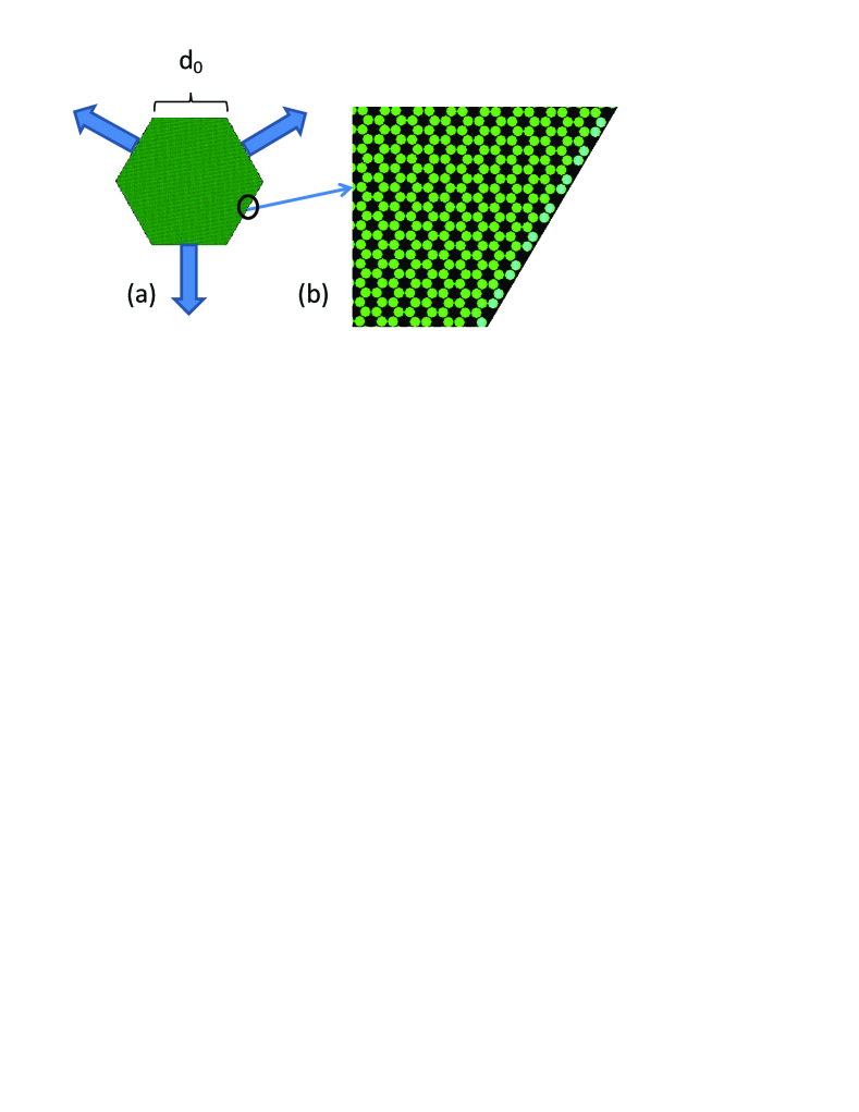
Figure 1: (Color online) (a) Hexagonal un-strained flake of graphene with armchair edges. The arrows in (a) indicate the triaxial strain directions. (b) The zoomed part of one of the edges.

Here both zig-zag and armchair hexagonal graphene flakes are studied separately. Notice that the three stressed edges (and also the free edges) should have only one type of edge: zig-zag or armchair. The zig-zag hexagonal flake is not shown in Fig. 1. In the following we present the methodology and compare our atomistic simulation results with those predicted by the above simple continuum elasticity theory.

III Molecular dynamics simulation with triaxial strain

We apply triaxial stress on the edges of an hexagonal flake of graphene as indicated in Fig. 1. Two different samples with armchair and zig-zag edges are considered and consist of 40234 and 40016 carbon atoms, respectively with optimized initial side i.e. $d_{0}=17.3$ nm. When applying stress, all atoms in the three none-alternative edges experience external constant force during each molecular dynamics simulation (MD) which causes them to move along the direction of the arrows shown in Fig. 1(a). The system reaches its equilibrium size under the applied force, resulting in different strains for different forces. In our MD simulations we have used the AIREBO potentialsStuart et al. (2000) which is in particular suitable for simulating hydrocarbons. The stretching process is done at low temperature (namely T=10 K). After reaching the desired strain (i.e. we study strains up to the breaking point) we performed energy minimization to find the minimum energy configuration using the conjugate gradient method under the constant force condition. We notice that there is no out-of-plane deformation in the final minimized samples. We consider a measure of the strain determined by $\epsilon=(d-d_{0})/d_{0}$ where $d$ is the distance between the center of the hexagonal flake and one of the edges under stress. The final strained samples are no longer perfect hexagons (see Fig. 2).

The applied stress changes the reciprocal lattice as well as the real space lattice. Using the two dimensional Fourier transformation of the final strained samples the change in the reciprocal lattice (Brillouin zone) is obtained. Figures 2(a,b,c) show the diffraction pattern of the original un-strained, strained zig-zag and armchair flakes, respectively where $\epsilon=13\%$. Notice that the original K and K^′ valleys are altered differently due to the in-plane triaxial strain. The variation in the diffraction pattern is different from that of corrugated suspended graphene due to intrinsic thermal ripplesMeyer et al. (2007). It is expected that such new patterns can be realized in experiment. The direct lattice and the reciprocal lattice deformations alter the hexagonal shape of the original Brillouin zone and will change the vector potentials Kitt et al. (2012); *kitt_erratum:_2013.

Figure 2: (Color online) Diffraction pattern for (a) un-deformed hexagonal flake (b) zig-zag (c) and armchair hexagonal flakes under triaxial stress.

IV Tight binding model for the gauge field

The electronic properties of graphene are described by a tight-binding Hamiltonian for the $\pi$ carbon orbitals. We employ the Hamiltonian that describes the low-energy band structureCastro Neto et al. (2009) ignoring the spin degrees of freedom which is motivated by the fact that no spin-flipping terms are present in the Hamiltonian. Strain is included in the modified hopping amplitudes between the $\pi$ orbitals, $t_{\pi}(r_{ij})$, according to the empirical relation $t_{\pi}(r_{ij})=t_{0}e^{-\beta(|\vec{\delta}_{ij}|/{a_{0}}-1)}$, where $\beta=-3.37$, $t_{0}=2.7eV$, $a_{0}=1.42$Å is the equilibrium inter-carbon distance and $\vec{\delta}_{ij}$ is the vector which connects the two neighboring atoms in the strained sample; here we consider both nearest and next-nearest neighbor terms. All neighbor distances are obtained from the relaxed MD sample. Since the applied strain is in-plane the effect of misalignment of the $\pi$ orbitals resulting from the finite curvature is negligible. More details of the used tight-binding model and the related numerical techniques for performing large system calculations can be found in our previous works Covaci and Peeters (2011); Covaci et al. (2010); Muñoz et al. (2012); *munoz_tight-binding_2013; Neek-Amal and Peeters (2012a).

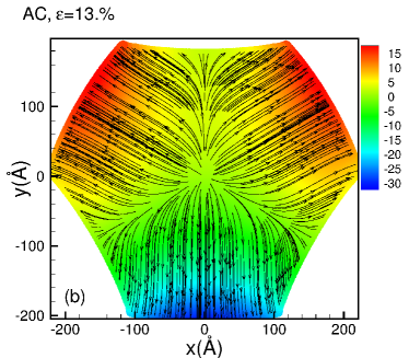
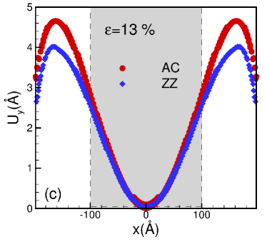
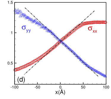
Figure 3: (Color online) The displacement vector pattern in strained (a) zig-zag (b) and arm-chair hexagonal graphene flakes. The variation of (c) $U_{y}$ versus $x$ where $|y|<2\,$Å  for zig-zag (circles) and armchair (triangles) hexagonal flakes subjected to an inhomogeneous strain of about $\epsilon=13\%$. In (d) the two diagonal elements of the stress tensor, i.e. $\sigma_{xx}$ and $\sigma_{yy}$ are compared to the prediction from elasticity theory (dashed lines) where $|y|<2\,$Å, see the text.

From a theoretical point of view, external forces deform graphene so that the nearest neighbor distances become non-equal and results in modified hopping parameters, which are now a function of the atomic positions $t(\textbf{r})$Neek-Amal et al. (2012); Castro Neto et al. (2009). The Fermi surface is displaced in reciprocal space ($\vec{k}\rightarrow\vec{k}-\frac{e}{\hbar}\vec{A}$), where $\vec{A}$ is the fictitious vector potential and $\vec{k}$ refers to the K-point) and consequently a pseudo-magnetic field ($\vec{B}=\frac{1}{e\,v_{F}}{\vec{\nabla}\times\vec{A}}$ where $e$ is the unit of charge and $v_{F}\sim 10^{6}m/s$ is the Fermi velocity in grapheneCastro Neto et al. (2009)) appearsLevy et al. (2010). The new term should be added to the original tight binding Hamiltonian due to the modification of the hopping parameters which includes the induced gauge field:

$$A_{x}+iA_{y}=\sum_{\vec{\delta}_{ab}}\delta t_{ab}(\vec{r})e^{-i\vec{k}.\vec{\delta}_{ab}},$$ (3)

where $\delta t_{ab}=t-t_{0}$ is the difference between the hopping parameters of the deformed and the original lattice. The position of the $\vec{K}$ valley in the original lattice is $\vec{K}=\frac{4\pi}{3\,a_{0}\sqrt{3}}(1,0)$ if the x-axis is taken along the zig-zag direction. We use Eq. (3) to calculate the pseudo-magnetic field which includes both changes in the hopping parameters and lattice deformations. As recently shown in Ref. [Sloan et al., 2013], this is the correct way to extract the pseudo-magnetic field from atomistic simulations.

Notice that one can use the displacement vectors given by Eq. (1) for producing a deformed hexagonal flake without molecular dynamics simulation relaxation. The latter can be used as the input coordinates for calculating the gauge field and the corresponding pseudo magnetic field. However we show in the appendix that the resulting Landau levels and the obtained lattice deformations are not consistent with those found here after fully relaxation of the coordinates using the true relaxation mechanism of the atomistic system.

V Results

V.1 Lattice deformation

In Fig. 3 we show the lattice deformation due to the triaxial strain (with $\epsilon=13\%$) in zig-zag terminated (a) and armchair terminated (b) hexagonal flakes, respectively. The arrows indicate the displacement vector streamlines, i.e. the vector field $\vec{U}$. In both cases the field refers to the triaxially stressed systems. The colors indicate the direction of the displacement vectors, i.e. red refers to upward and blue refers to downward displacements. The displacement vectors in zig-zag and armchair flakes are similar but the electronic properties will be rather different. The streamline vectors are perpendicular to the three stressed edges and are almost parallel to the free arc-shape edges. The larger the strain the larger the concavity of the edges.

In order to compare our numerical results with those predicted by Eq. (1), we plot the $U_{y}$ components of the resulted displacements from our MD simulations and the two main components of the stress tensor in panels (c) and (d) of Fig. 3. In Fig. 3(c) we show the variation of $U_{y}$ with $x$ for constant $y$ (i.e. $|y|<2$Å) in the strained armchair (blue diamonds) and zig-zag (red circles) which were subjected to the strain $\epsilon=13\%$. There is a clear deviation from linear behavior (see $U$ in Eq. (1)) which is very pronounced close to the borders of the sample. The same behavior is found for $U_{x}$ but is not shown. In Fig. 3(d) we show the variation of $\sigma_{yy}$ and $\sigma_{xx}$ with $x$ for a typical strain ($13\%$). The lines indicate the stress component from Eq. (2). It is again seen that there is considerable deviation from the prediction of continuum elasticity theory (Eq. (1)), in particularly beyond $|x|>$50Å  where the zig-zag and armchair profiles deviate from each other; notice that linear elasticity theory does not distinguish these two different lattice orientations. The reason for these deviations is the effect of the free edges on the lattice distortion which results in a complex strain distribution. The latter effect was neglected in the previous studiesGuinea et al. (2009); Vozmediano et al. (2010). Nevertheless, in most recent theoretical works the main attention was directed to the center of the flake which as we see from Figs. 3(c,d), for the region $|x|<50\,$Å,   agrees with elasticity theory.

V.2 Pseudo-magnetic field

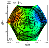
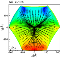
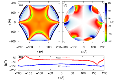
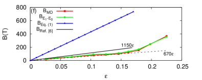
Figure 4: (Color online) Vector potential $\vec{A}$ for strained hexagonal zig-zag (a) and armchair (b) graphene where $\epsilon=13\%$. The corresponding pseudo-magnetic field is shown in (c) for zig-zag and (d) armchair flakes. (e) The pseudo-magnetic field profile along the $x$-axis for both armchair (red square) and zig-zag (blue cricles) flakes. (f) Comparison between the pseudo-magnetic field at the center of the zig-zag flake obtained from the deformation (red squares), from the electronic gap between the zero and first pseudo-Landau levels (green circles) and the prediction from linear elasticity theory given by Ref. [Guinea et al., 2009](blue triangles).

Using Eq. (3) we calculated the vector potential for the obtained lattice deformations from our MD simulations. It is interesting that the vector potential streamlines exhibit neither constant nor circular orbits. In the zig-zag flake the vector potential shows orbits having deformed triangular shape (there is a kind of three fold symmetry, see Fig. 4(a)) but surprisingly for the armchair flake they do not exhibit orbits and the vectors follow an hyperbolic function, Fig. 4(b). Therefore the corresponding pseudo-magnetic field for the two cases will be very different. The pseudo-magnetic field profiles as generated by the strain configurations are shown in Figs. 4(c) and 4(d) for the zig-zag and armchair flakes, respectively. The important effect is the variation of the field over the zig-zag flake, specially around the center of the flake (see Appendix B). For the armchair flake the induced magnetic field is close to zero and varies smoothly in the central part, see Fig. 4(d). For better visualization we plot in Fig. 4(e) the pseudo-magnetic field along the arrows shown in Figs. 4(c,d). It is interesting to note that the pseudo-magnetic field in the zig-zag flake exhibits three fold symmetry while for the armchair it shows a more complex pattern. We also present in Fig. 4(f) a comparison between the central pseudo-magnetic fields obtained directly from the deformation, the field obtained from the electronic gap between the zeroth and first pseudo-Landau levels and the prediction from Ref. [Guinea et al., 2009], and that of resulted using Eq. (1) ,i.e. $B=\frac{16\,C\,\hbar}{a_{0}\,e}$. A linear regime is found only for $\epsilon<15\%$, while beyond this value the pseudo-magnetic field behaves non-linearly with respect to $\epsilon$. The values obtained from the deformation and electronic properties are very similar but much smaller than the prediction of continuum elasticity theory (triangular symbols in Fig. 4(f)). We attribute this discrepancy to the change in the lattice structure due to the relaxation of the graphene sheet. We note that for the same $\epsilon$ the shape of the flake obtained from the MD simulation is very different from the one obtained from the deformation defined by Eq. (1).

V.3 Local density of states

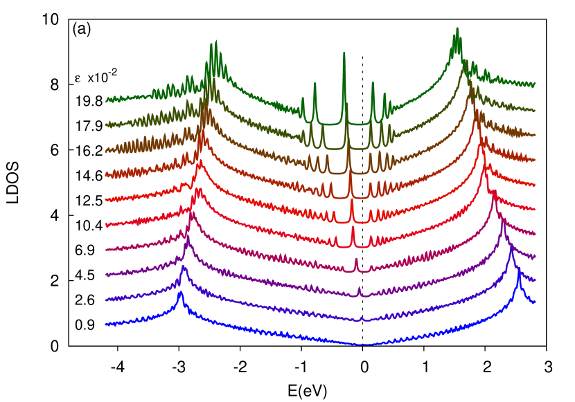
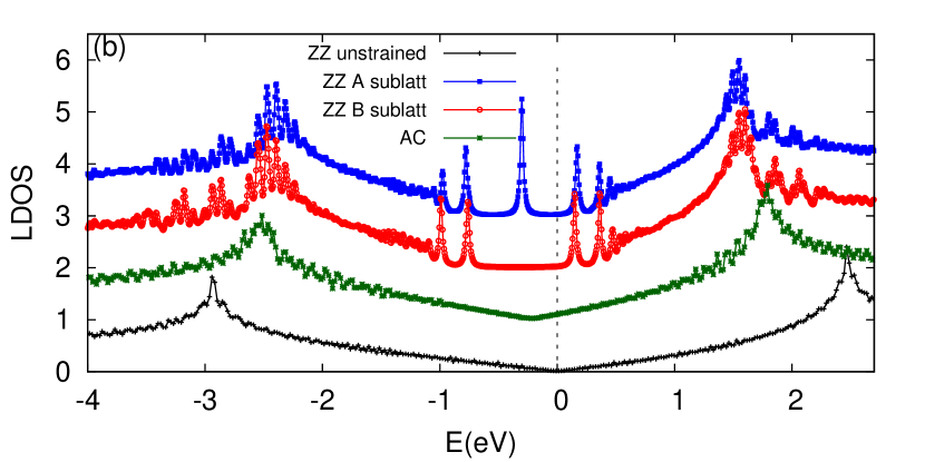
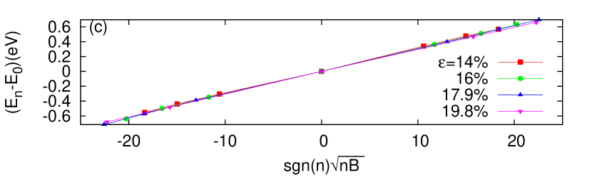
Figure 5: (Color online) (a) Local density of states in the center of the hexagon for the A-sublattice and various strains. (b) Comparison between the central LDOS of the unstrained zig-zag flake, strained zig-zag flake for both A and B sublattices and strained armchair flake with strain of 13$\%$. (c) Plot of the positions of the pseudo-Landau levels versus $sgn(n)\sqrt{nB}$, where $B$ is extracted from the difference between the position of the zeroth and first Landau level. Note that the energy is shifted such that the Dirac point of the unstrained configuration sits at the Fermi level.

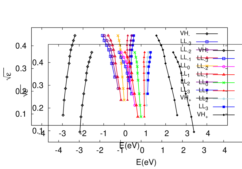
Figure 6: (Color online) Plot of the energies corresponding to the lower and higher van Hove singularities and the pseudo-Landau levels, $n=\pm 3,\pm 2,\pm 1,0$, as a function of $\sqrt{\epsilon}$ obtained from the peaks in the LDOS at the center of zig-zag strained hexagon.

In order to investigate the effect of strain on the electronic properties, we input the relaxed atomic positions obtained from our atomistic simulation into a real-space tight-binding model. Our main focus in this work is to find the LDOS maps, which could be directly accessed by STM experiments. The LDOS maps are obtained by expanding the Green’s function at each atomic position in terms of Chebyshev polynomials . The details of this expansion can be found in our previous works Covaci and Peeters (2011); Covaci et al. (2010); de Juan et al. (2012); Muñoz et al. (2012); *munoz_tight-binding_2013. Here we use both nearest neighbor and next-nearest neighbor contributions in the tight-binding Hamiltonian in order to account both for the strain induced vector potential (nearest neighbor) and the strain induced scalar potential (next-nearest neighbor).

First, in Fig. 5(a), we show the LDOS for an atom in the A-sublattice (which are under stress at the three edges) in the center of the hexagon for various applied force strengths. Several interesting effects can be observed. Because we also include next-nearest neighbor hopping amplitudes in the calculation, the Dirac point for the unstrained hexagon sits at a finite energy, $E_{D}=3\,t^{\prime}$, where $t^{\prime}$ is the next-nearest neighbor hopping amplitude. We therefore shift all the LDOS curves such that the Dirac point of the unstrained configuration sits at the Fermi level. We also observe an additional shift for the strained configurations because of the exponential suppression in $t^{\prime}$, which could be understood in terms of a strain induced scalar potential, which shifts the Dirac point downwards in energy Castro Neto et al. (2009). In addition, the reduction in the hopping amplitudes shift the van-Hove peaks, signaling also a change in the Fermi velocity. Another important effect, noted already in Ref. [Guinea et al., 2009], is the appearance of peaks in the LDOS for the strained zig-zag hexagon. These correspond to pseudo-Landau levels generated by the strong pseudo-magnetic field observed in the central region of the zig-zag hexagon. When compared to the regular Landau levels generated by real magnetic fields, one important difference can be seen: we find that the zeroth Landau level has a finite contribution to the LDOS only in one sub-lattice, i.e. the sublattice pertaining to the edge atoms under stress. For the non-zero pseudo-Landau levels the sublattice symmetry still holds. This can be seen in Fig. 5(b) where we show the LDOS in the center of the strained hexagon (with $\epsilon=13\%$) for the A and B sub-lattice and compare them with the LDOS for the unstrained zig-zag case and the LDOS in the center of the strained armchair hexagon. Since the pseudo-magnetic field at the center of the armchair hexagon is small, the LDOS does not show pseudo-Landau levels, but shows a strain induced shift of both the Dirac point and the van Hove peaks.

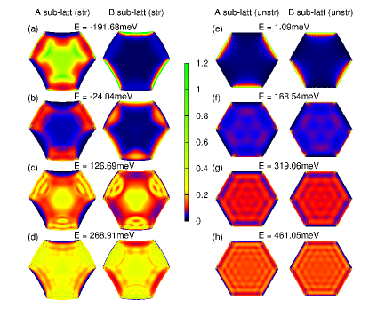
Figure 7: (Color online) LDOS maps for a strained zig-zag hexagon with $\epsilon=13\%$, panels (a)-(d), and for an unstrained one, panels (e)-(h). Panel (a) corresponds to the zero pseudo-Landau level, while panels (c) and (d) correspond to the first and second pseudo-Landau levels, respectively.

The relativistic nature of the pseudo-Landau levels is clearly apparent from Fig. 5(c), where we plot the energy of the pseudo-Landau levels for different strains as a function of $sgn(n)\sqrt{nB}$. Note that we shift the pseudo-Landau levels such that the zero-Landau level sits at zero energy. Surprisingly, the relationship is linear. Note that the pseudo-magnetic field (also shown in Fig. 4(f)) was extracted from the energy gap between the zero and first pseudo-Landau levels by using a constant Fermi velocity and the known relationship: $E_{1}=\sqrt{2e\hbar v_{F}^{2}B}\approx 30meV\sqrt{B(Tesla)}$. Even though for low strains the pseudo-magnetic field is proportional to $\epsilon$, the suppression of the Fermi velocity (signaled by the shift of the van Hove peaks) will lead to a non-linear dependence of the energy of the pseudo-Landau levels on $\sqrt{\epsilon}$. This becomes more drastic at high strains, where the pseudo-magnetic field does not follow anymore a linear relationship with respect to $\epsilon$ (see Fig. 4(f)). This can be seen more clearly in Fig. 6, where the energies of the van Hove peaks and of the pseudo-Landau levels are plotted as a function of $\sqrt{\epsilon}$. Although the spectrum of the unstrained graphene is not particle-hole symmetric, we fined that in the zig-zag strained graphene samples the higher-n pseudo-Landau levels are symmetric with respect to the zeroth pseudo-Landau level.

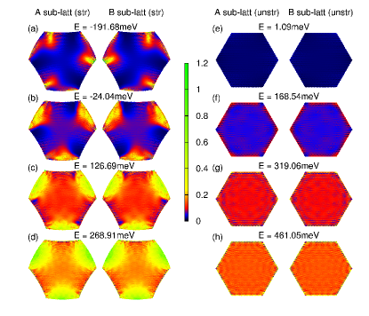
Figure 8: (Color online) LDOS maps for a strained armchair hexagon with $\epsilon=13\%$, panels (a)-(d), and for an unstrained one, panels (e)-(h).

Next we show in Fig. 7 the LDOS maps for various energies for a strained zig-zag hexagon with $\epsilon=13\%$. The contributions to each sub-lattice are plotted separately for clarity. In panels (a)-(d) we show the LDOS for the strained configuration, while in panels (e)-(h) the LDOS for the unstrained zig-zag hexagon is shown for corresponding energies. The energy of the LDOS map in panel (a) corresponds to the energy of the zero Landau level. We observe a large increase in the LDOS in sub-lattice A (which are under stress at the three edges) in the regions where the pseudo-magnetic field is large, together with a suppression of the LDOS in sub-lattice B. This effect shows the most important difference between pseudo-magnetic fields and real magnetic fields. Since a gap appears in the spectrum, and the time-reversal symmetry is not broken, this is a clear manifestation of a broken sub-lattice symmetry. If the hexagon would be pulled from the other three sides, the pseudo-magnetic field would change sign and the zero pseudo-Landau level will appear in the other sub-lattice.

The LDOS map shown in Fig. 7(b) corresponds to an energy close to the Dirac point of the unstrained configuration. The only noticeable contributions come from the edge-like states, which are again seen only in sub-lattice A. The energies of the LDOS maps shown in Fig. 7(c) and 7(d) correspond to the energies of the first and second pseudo-Landau levels, respectively. In this case, we observe that the sub-lattice symmetry is preserved in the central region of the hexagon. For these energies the real and pseudo-Landau levels are similar. Interesting features appear also at energies near the van Hove peaks, for which the LDOS maps show resonant peaks at the center of the hexagon. At these energies peaks start developing, while there is no broken sub-lattice symmetry. It is important to note that the low energy theory which relates the strain to a pseudo-vector potential is not valid near the van Hove peaks mainly because the dispersion is not linear anymore. Movies of the LDOS maps for all energies are presented as Supplementary Materials .

Next we show for comparison in Fig. 7(e)-(h) the LDOS maps for the unstrained zig-zag hexagon. Due to the symmetries of the system, i.e. $\pi/3$ rotational symmetry, the boundary conditions are such that the wave-function is zero in sub-lattice A in three non-consecutive sides and zero in sub-lattice B in the other three sides. At the Dirac point, panel (e), edge states with zero energy appear and are located in different sub-lattices on different sides of the hexagon. For all energies the LDOS map for the A sub-lattice is the same as the one for the B sub-lattice but rotated are $\pi/3$, as expected due to symmetry arguments.

The LDOS maps for the armchair hexagon are presented in Fig. 8, both for the strained, panels (a)-(d), and the unstrained configurations, panels (e)-(h). The boundary condition now sets the wave-function to zero in both sub-lattices at all hexagon edges. The main symmetry, which is preserved also in the strained configuration is the mirror symmetry plus a sub-lattice exchange with respect to $x=0$. The effect of strain on the LDOS maps is not so drastic as the one for the zig-zag hexagon. Besides the overall shift in energy due to the appearance of the scalar gauge field, the main modifications can be seen only at the edges of the hexagon where the pseudo-magnetic field is large. Since the field changes sign, we see localization of states at the Dirac point in both A and B sub-lattices.

VI Summary

In this paper we studied the effect of triaxial stress on the electronic and structural properties of hexagonal flakes of graphene with zig-zag and armchair edges. We combined molecular dynamics simulations to obtain the relaxed atomic positions and the tight binding method to describe the electronic properties. We found that lattice deformations under triaxial stress are well described by continuum elasticity theory only for small strains ($\epsilon<15\%$) and only in the central part of the sample. The pseudo gauge field was found to be neither circular symmetric nor homogeneous in space, i.e. there are modified triangular orbits for zig-zag flakes and none-orbital vectors for armchair flakes when the deformed lattice is fully relaxed. The corresponding pseudo-magnetic field is non-uniform over the sample and exhibits three fold symmetry for a zig-zag flake and a more complex variation for the armchair flake. Only for zig-zag flakes we find that in the central region the pseudo-magnetic field is large and while it varies significantly near the edges, while for the armchair flakes the field is very small in the center and oscillating near the edges. The local density of states are completely different at the different sub-lattices and are mostly affected by the pseudo-magnetic field distribution. In the zig-zag hexagon the appearance of pseudo-Landau levels breaks the sub-lattice symmetry in the zeroth pseudo-Landau level and all relaxed samples show a shift in the energy levels as compared to the undeformed case due to the appearance of a strain induced scalar potential resulting from the expansion of the graphene flake. We find that molecular dynamics relaxation changes strongly the pseudo-magnetic field and the local density of states as compared to the deformed none-relaxed samples from elasticity theory. The latter shows that relaxation of the atomistic structure of the deformed graphene under constraints plays an important role in the electronic properties and that predictions of elasticity theory applicable for continuum sheets should be modified, especially for large strains.

Appendix A Effect of lattice relaxation

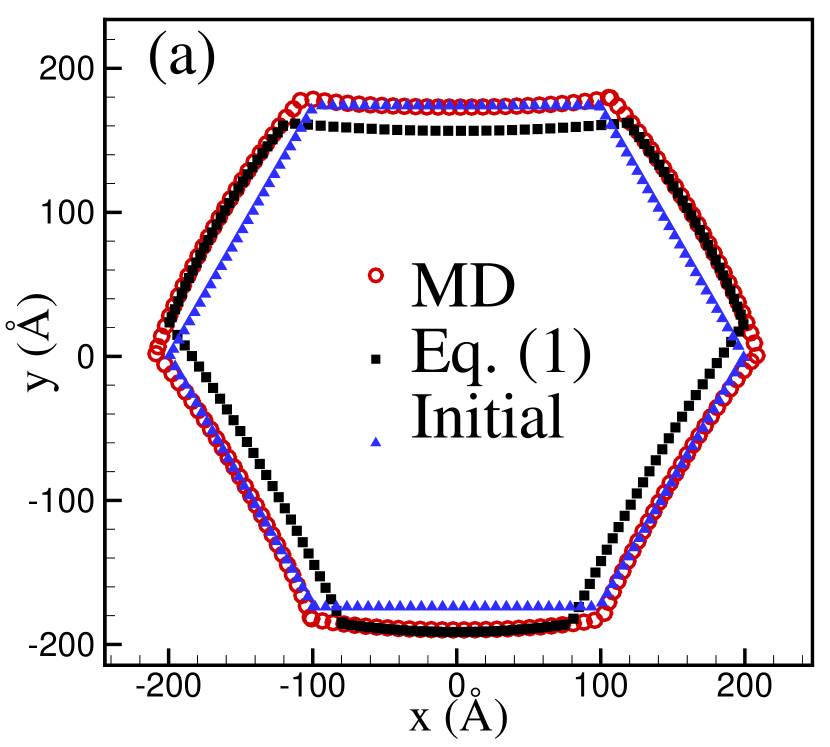
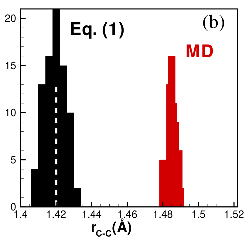
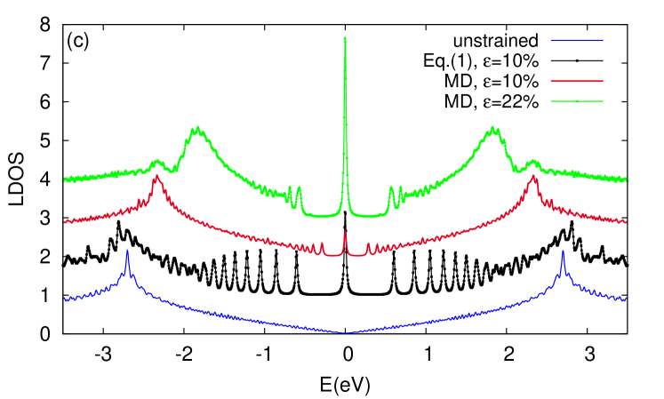
Figure 9: (Color online) (a) The boundary of the deformed lattice using Eq. (1) (black squares), MD relaxed flake (red circles) and undeformed lattice (blue triangles) for a hexagonal flake subjected to a strain of 10$\%$. (b) The C-C bond length histogram in the case of MD relaxation and using Eq. (1) which is the method used in Ref. [6]. (c) Comparison between the central LDOS of the unstrained zig-zag flake (blue curve), strained zig-zag flake for strain 22$\%$ (green curve) and 10$\%$ (red line) and that obtained by using deformation based on Eq. (1) (black curve).

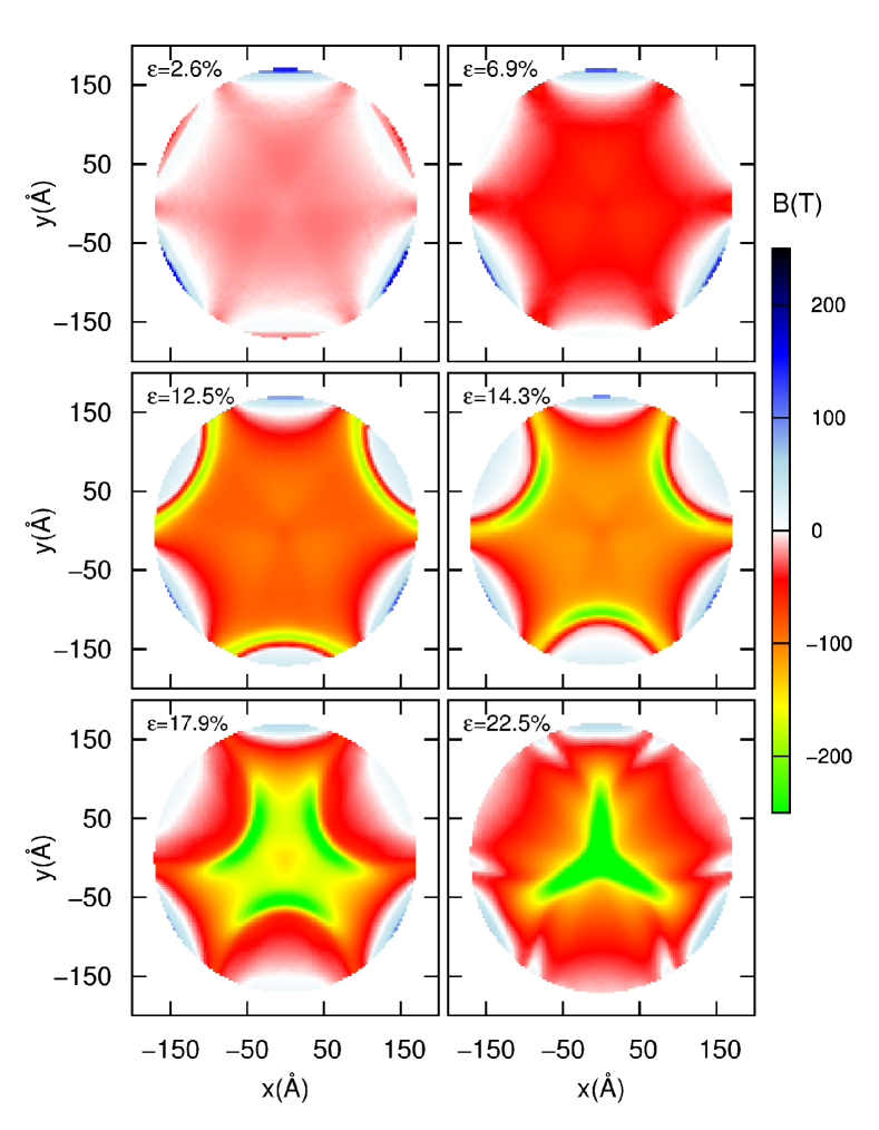
Figure 10: (Color online) The effect of strain on the pseudo-magnetic field in the central part of the zig-zag hexagonal graphene flake, $|\textbf{r}|<17$ nm.

In this appendix we discuss the important effect of the atomistic relaxation of nano-scale samples using bond order force field on the electronic properties of the studied hexagonal graphene flakes. One of the simplest way to deform the perfect graphene lattice non-uniformly (blue triangle in Fig. 9) is by using directly Eq. (1) (here the case of triaxial strain). The boundary of the resulting deformation for hexagonal graphene zig-zag flake subjected to 10$\%$ strain is shown in Fig.  9(a), see black square symbols. The corresponding result obtained when using the MD relaxation is shown as open red circles in Fig. 9(a). As obviously from the figure, the MD relaxation expands the area of flake, thus one expects longer C-C bond lengths. In order show the latter effect we plotted in Fig. 9(b) the histogram of C-C bond lengths in the central part ($|\textbf{r}|<$5Å) of hexagonal flakes for the two before mentioned methods. The shorter the bond lengths, the more compact the lattice and the higher the local stress in the central part will be, which results in higher pseudo-magnetic field, see blue triangles and red squares in Fig. 4(f) (see the results for triaxial stressed unrelaxed hexagonal flake in Ref. Ramezani Masir et al. which are more than ten times higher than those we report here). In order to reveal the large difference between the pseudo-magnetic fields and the consequent effects on the electronic spectrum we depicted in Fig. 9(c) the LDOS for two relaxed systems by MD method for $\epsilon=10\%,22\%$, a deformed system with $\epsilon=10\%$ (black curve) by using Eq. (1) and an undeformed hexagonal flake. Here we use only the nearest-neighbor hopping amplitudes since the only effect of the next-nearest neighbor term is to shift the Dirac point. The position of the pseudo-Landau levels and the shift of the van Hove peaks are not affected by the change in the next-nearest neighbor hopping. In the case of an undeformed sample (ordinary hexagonal flake shown by blue triangles in Fig. 9(a)), we see that there is no zero energy state at the Dirac point. By deforming the lattice following Eq. (1) with $\epsilon=10\%$ (hexagonal flake shown by black squares in Fig. 9(a)) pseudo-Landau levels with energy separation proportional to $\sqrt{n}$ appear for both electrons and holes. The MD relaxation changes significantly the LDOS profiles because of the mentioned lattice expansion. First, we observe that for the same deformation, $\epsilon=10\%$, the gap between the zero and first pseudo-Landau levels is much smaller, consistent with a much lower pseudo-magnetic field. We also find that fewer pseudo-Landau levels can be distinguished, even at high strains, e.g. $\epsilon=22\%$. This could be a consequence of the fact that at high strains the pseudo-magnetic field for the MD relaxed system is not constant, and therefore the high-$n$ pseudo-Landau levels are smeared out.

Appendix B Effect of strain on pseudo-magnetic field

Here we show the effect of strain on the pseudo-magnetic field for different strains in zig-zag hexagonal graphene flakes. The larger the strain the larger the pseudo-magnetic field. In Fig.  10 we show the pseudo-magnetic field for strains in the range of [2.6$\%$-22.5$\%$] in the central region, i.e $|\textbf{r}|<17$ nm. It is seen that in the central portion of the zig-zag hexagonal graphene flakes the pseudo-magnetic field is not constant which is in contrast to the continuum elasticity theory prediction [6], and the result obtains from Eq. (1), $B=\frac{16\,C\,\hbar}{a_{0}\,e}$.

Appendix C Alternative methods for applying stress on the edges

In addition to the method for applying the stress presented here, one can fix the boundary atoms and shift them gradually in the direction perpendicular to the edges. Since the boundary atoms are not allowed to be relaxed during the simulation, the inter-atomic distances at the edge remain constant giving high stress at the corners, which consequently affects the stress distribution through the system. The latter effect modifies both the pseudo-magnetic field and the LDOS. We found that in case of such a fixed boundary condition the pseudo-magnetic field is higher than the one found from the constant applied force method, as shown in Figs. 11(a-d). Moreover, the pseudo-magnetic is also more inhomogeneous. The recent experimental realization of triaxial strain in molecular graphene Gomes et al. (2012) confirms that the method used in the present work is realistic. The constant motion of the edges was recently used by Z. Qi et al. in order to study the resonant tunneling in hexagonal graphene Qi et al. quantum dots. This should be modified in order to have the relevant order of magnitude of the pseudo-magnetic field and consequently the correct position of the Landau levels.

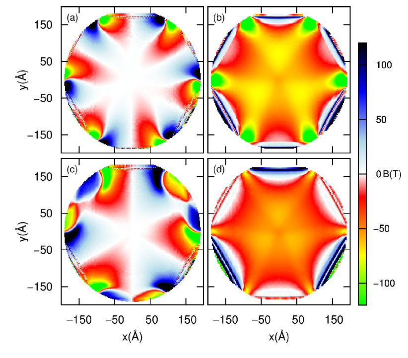
Figure 11: (Color online) Pseudo-magnetic field in the central part of the arm-chair (a),(c) and zig-zag (b),(d) hexagonal graphene flake, $|\textbf{r}|<17$ nm where $\epsilon=13\%$. The fields are obtained either by moving the edges (a),(b) or by applying a constant force on the edges (c),(d).

References

- Gomes et al. (2012) K. K. Gomes, W. Mar, W. Ko, F. Guinea, and H. C. Manoharan, Nature (London) 483, 306 (2012).
- Pereira et al. (2009) V. M. Pereira, A. H. Castro Neto, and N. M. R. Peres, Phys. Rev. B 80, 045401 (2009).
- Castro Neto et al. (2009) A. H. Castro Neto, F. Guinea, N. M. R. Peres, K. S. Novoselov, and A. K. Geim, Rev. Mod. Phys. 81, 109 (2009).
- Guinea et al. (2010) F. Guinea, A. K. Geim, M. I. Katsnelson, and K. S. Novoselov, Phys. Rev. B 81, 035408 (2010).
- Fogler et al. (2008) M. M. Fogler, F. Guinea, and M. I. Katsnelson, Phys. Rev. Lett. 101, 226804 (2008).
- Guinea et al. (2009) F. Guinea, M. I. Katsnelson, and A. K. Geim, Nat Phys 6, 30 (2009).
- Levy et al. (2010) N. Levy, S. A. Burke, K. L. Meaker, M. Panlasigui, A. Zettl, F. Guinea, A. H. C. Neto, and M. F. Crommie, Science 329, 544 (2010).
- Low and Guinea (2010) T. Low and F. Guinea, Nano Lett. 10, 3551 (2010).
- Vozmediano et al. (2010) M. Vozmediano, M. Katsnelson, and F. Guinea, Physics Reports 496, 109 (2010).
- Yamamoto et al. (2012) M. Yamamoto, O. Pierre-Louis, J. Huang, M. S. Fuhrer, T. L. Einstein, and W. G. Cullen, Phys. Rev. X 2, 041018 (2012).
- Klimov et al. (2012) N. N. Klimov, S. Jung, S. Zhu, T. Li, C. A. Wright, S. D. Solares, D. B. Newell, N. B. Zhitenev, and J. A. Stroscio, Science 336, 1557 (2012).
- Goerbig et al. (2008) M. O. Goerbig, J.-N. Fuchs, G. Montambaux, and F. Piéchon, Phys. Rev. B 78, 045415 (2008).
- Montambaux et al. (2009) G. Montambaux, F. Piéchon, J.-N. Fuchs, and M. O. Goerbig, Phys. Rev. B 80, 153412 (2009).
- (14) M. Ramezani Masir, D. Moldovan, and F. M. Peeters, arXiv:1304.0629(2013), to appear in Solid State Comm. .
- Neek-Amal and Peeters (2012a) M. Neek-Amal and F. M. Peeters, Phys. Rev. B 85, 195445 (2012a).
- Neek-Amal and Peeters (2012b) M. Neek-Amal and F. M. Peeters, Phys. Rev. B 85, 195446 (2012b).
- Kitt et al. (2012) A. L. Kitt, V. M. Pereira, A. K. Swan, and B. B. Goldberg, Phys. Rev. B 85, 115432 (2012).
- Kitt et al. (2013) A. L. Kitt, V. M. Pereira, A. K. Swan, and B. B. Goldberg, Phys. Rev. B 87, 159909 (2013).
- de Juan et al. (2012) F. de Juan, M. Sturla, and M. A. H. Vozmediano, Phys. Rev. Lett. 108, 227205 (2012).
- Linnik (2012) T. L. Linnik, J. Phys.: Condens. Matter 24, 205302 (2012).
- (21) M. Neek-Amal, J. Beheshtian, A. Sadeghi, K. H. Michel, and F. M. Peeters, To appear in J. Phys. Chem. C http://dx.doi.org/10.1021/jp402122c (2013).
- Heiskanen et al. (2008) H. P. Heiskanen, M. Manninen, and J. Akola, New J. Phys. 10, 103015 (2008).
- Zhang et al. (2008) Z. Z. Zhang, K. Chang, and F. M. Peeters, Phys. Rev. B 77, 235411 (2008).
- Zarenia et al. (2011) M. Zarenia, A. Chaves, G. A. Farias, and F. M. Peeters, Phys. Rev. B 84, 245403 (2011).
- (25) Z. Qi, D. Bahamon, V. Pereira, H. Park, D. Campbell, and A. Castro Neto, to appear in Nano Letters .
- Stuart et al. (2000) S. J. Stuart, A. B. Tutein, and J. A. Harrison, J. Chem. Phys. 112, 6472 (2000).
- Meyer et al. (2007) J. C. Meyer, A. K. Geim, M. I. Katsnelson, K. S. Novoselov, T. J. Booth, and S. Roth, Nature (London) 446, 60 (2007).
- Covaci and Peeters (2011) L. Covaci and F. M. Peeters, Phys. Rev. B 84, 241401 (2011).
- Covaci et al. (2010) L. Covaci, F. M. Peeters, and M. Berciu, Phys. Rev. Lett. 105, 167006 (2010).
- Muñoz et al. (2012) W. A. Muñoz, L. Covaci, and F. M. Peeters, Phys. Rev. B 86, 184505 (2012).
- Muñoz et al. (2013) W. A. Muñoz, L. Covaci, and F. M. Peeters, Phys. Rev. B 87, 134509 (2013).
- Neek-Amal et al. (2012) M. Neek-Amal, L. Covaci, and F. M. Peeters, Phys. Rev. B 86, 041405 (2012).
- Sloan et al. (2013) J. V. Sloan, A. A. P. Sanjuan, Z. Wang, C. Horvath, and S. Barraza-Lopez, Phys. Rev. B 87, 155436 (2013).
- Note (1) Movies of the LDOS maps for the whole spectrum are presented as Supplementary Materials.