Plasmons in a Superlattice of Fullerenes or Metallic Shells

Abstract

A theory for the collective plasma excitations in a linear periodic array of spherical two-dimensional electron gases (S2DEGs) is presented. This is a simple model for an ultra thin and narrow microribbon of fullerenes or metallic shells. Coulomb coupling between electrons located on the same sphere and on different spheres is included in the random-phase approximation (RPA). Electron hopping between spheres is neglected in these calculations. The resulting plasmon-dispersion equation is solved numerically. Results are presented for a superlattice of single-wall S2DEGs as a function of the wave vector. The plasmon dispersions are obtained for different spherical separations. We show that the one-dimensional translational symmetry of the lattice is maintained in the plasmon spectrum. Additionally, we compare the plasmon dispersion when the superlatice direction is parallel or perpendicular to the axis of quantization. However, because of anisotropy in the Coulomb matrix elements, there is anticrossing in the plasmon dispersion only in the direction perpendicular to the quantization axis. The S2DEG may serve as a simple model for fullerenes, when their energy bands are far apart.

I Introduction

Research on the properties of carbon-based materials has soared over the years mainly because it may be found in a variety of allotropic forms. These include graphite, graphene, carbon nanotubes and nanoscrolls as well as fullerenes. In particular, the discovery of fullerenes O1 ; O1b ; O2 ; O3 ; O4 ; O5 ; O6 has led to several impressive advances in the study of carbon nanoparticles XXX1 . The optical properties of fullerenes have been investigated from both an experimental and theoretical point of view EELS ; Apell ; expt1 ; expt2 . Since optical measurements are a non-invasive probe of the samples, they provide reliable information about the electronic properties of fullerenes.

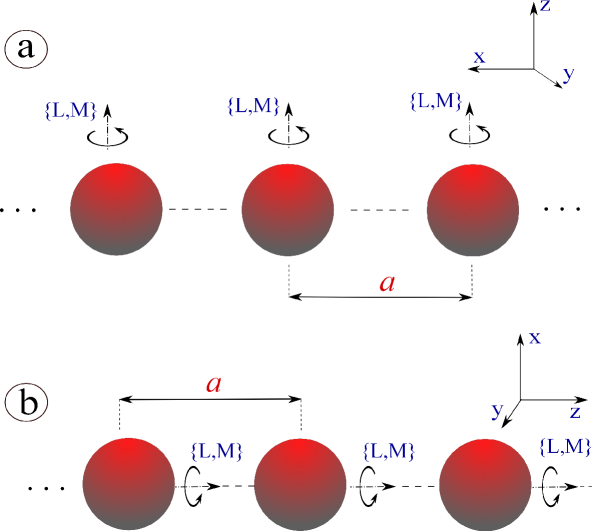
Figure 1: (Color online) Schematic representation of a superlattice of spherical two-dimensional electron gases (a) perpendicular and (b) along the axis of quantization.

As a result of the recent advances in techniques such as solvent-assisted self-assembly XXX2 , fullerenes can now be produced in abundant quantities even to form thin films of fullerene-like MoS nanoparticles XXX3 and have stimulated renewed interest in these materials. Additionally, the ability to control optical fields has now made it feasible to ascertain the plasmon excitations in pre-arranged arrays of fullerenes XXX2 ; XXX3 . We consider a simple model for an ultra narrow and thin film of fullerenes forming a microribbon by employing a one-dimensional superlattice. In this work, we investigate the photoexcitation of plasmons in a regular periodic array of fullerenes shown schematically in Fig. (1). Our goal is to thoroughly analyze the dependence of the plasma frequency on the relative orientation of the EM probe field with respect to the axis along which the periodicity occurs.

We demonstrate that the optical absorption spectra of such nano spheres exhibit a rich dependence on the magnitude and direction of the transfer momentum. The wave functions have spatial symmetry originating from those of the individual fullerenes. Therefore, the natural first step is to specify the model which we employ for each buckyball. For simplicity and ease of mathematical analysis, but at the same time retaining essential geometrical characteristics, we assume that an electron gas is confined to the surface of a sphere of chosen radius Inaoka ; Devreese ; Yannouleas . This spherical two-dimensional electron gas (S2DEG) is characterized by the electron effective mass $m^{\ast}$ and the number $N_{F}$ of occupied energy levels. Our model enables us to exploit spherical symmetry of the particulates in the Bloch-Floquet theorem for generating the wave functions in a linear array aizin . This effective mass model is suitable for “small” nano spheres, i.e., when the separation between energy levels is large. Additionally, the energy band structure may be included into our formalism through form factors for the Coulomb matrix elements and the polarization function. In this regard, we note that electron energy loss spectroscopy (EELS) has been used to probe the plasmon excitations for concentric-shell fullerenes embedded in a film EELS . Furthermore, perfectly spherical shells were used in the theoretical modeling of the EELS data and the agreement was good. The model of Lucas, et al. Lucas . was shown to be qualitatively adequate for understanding the optical data for multi-shell fullerenes. In that work Lucas , the ultraviolet dielectric tensor of monolayer graphene is adapted to the spherical geometry of a fullerene by averaging over the three possible orientations of the ${\bf c}$ axis. Thus, a continuum model was used by Lucas, et al. Lucas starting from the planar local dielectric function of planar monolayer graphene.

The rest of this paper is organized as follows. Section II contains our theoretical framework and the results based on it. Illustrative comparisons with data sets are given there as well. The last section, Sec. III, is devoted to a short summary and relevant comments.

II General Formulation of the Problem

Let us consider a linear array of spherical two-dimensional electron gases, with their centers located on the $x$ axis. The center of each shell is at $x=na$ ($n=0,\pm 1,\pm 2,\cdots$). Each “ball” consists of $N$ concentric shells with radii $R_{1}<R_{2}<\cdots<R_{N}$, where $a>2R_{N}$. For simplicity, we assume that each spherical shell is infinitesimally thin. We will construct the electron wave functions in the form of Bloch combinations as described by Huang and Gumbs for an array of rings huangandgumbs and by Gumbs and Aizin for an array of cylinders aizin . In the absence of tunneling between the shells, the single-particle Bloch wave functions for the array with the periodicity of the lattice are given by

$$<{\bf r}|\nu>=\frac{1}{N_{x}}\sum_{j=-\frac{N_{x}}{2}}^{\frac{N_{x}}{2}}e^{ik_{x}ja}\Psi_{lm}(\vec{r}-ja\hat{e}_{x})\ ,\ \ \ \Psi_{lm}(\vec{r}-ja\hat{e}_{x})=\frac{\mathcal{R}_{j}(r)}{R}Y_{lm}(\Omega),\ \ \$$ (1)

where $\nu=\{k_{x},l,m\}$ is a composite index for the electron eigenstates, $\Psi_{lm}(\vec{r})$ is the wave function for an electron, with angular momentum quantum numbers $l=0,1,2,\cdots$ and $|m|\leq l$, $\mathcal{R}_{j}^{2}(r)=\delta(r-R_{j})$. Additionally, $k_{x}=\frac{2\pi}{L_{x}}n$ with $n=0,\pm 1,\pm 2,\cdots,\pm\frac{N_{x}}{2}$. Here, $N_{x}=L_{x}/a$ is the number of nano balls in the array with periodic boundary conditions. Electron motion in the azimuthal direction around the shells is quantized and characterized by the angular momentum quantum number $l$. The electron spectrum in each shell is discrete and given by $\epsilon_{\nu}=\hbar^{2}l(l+1)/2\mu^{\ast}R^{2}$ . The spectrum does not depend on $m$ and $k_{x}$.

Plasmons may be obtained from the solution of the density matrix equation, as described above. We have

$\displaystyle{i\hbar\frac{\partial\hat{\rho}}{\partial t}=[\hat{{\cal H}},\hat{\rho}]}$ aizin . For $\hat{{\cal H}}=\hat{{\cal H}}_{0}-e\tilde{\varphi}$ and $\hat{\rho}=\hat{\rho}_{0}+\delta\hat{\rho}$, with $<i\nu|\hat{{\cal H}}_{0}|i^{\prime}\nu^{\prime}>=\epsilon_{i\nu}\delta_{\nu\nu^{\prime}}\delta_{ii^{\prime}}$, $<i\nu|\hat{\rho}_{0}|i^{\prime}\nu^{\prime}>=2f_{0}(\epsilon_{i\nu})\delta_{\nu\nu^{\prime}}\delta_{ii^{\prime}}$, we obtain in the lowest order of perturbation theory

$$<i\nu|\delta\hat{\rho}|i^{\prime}\nu^{\prime}>=2e\ \frac{f_{0}(\epsilon_{\nu})-f_{0}(\epsilon_{\nu^{\prime}})}{\hbar\omega-\epsilon_{\nu}+\epsilon_{\nu^{\prime}}}<i\nu|\tilde{\varphi}({\bf r})|i^{\prime}\nu^{\prime}>\ ,$$ (2)

where $f_{0}(\epsilon)$ is the Fermi function and $\tilde{\varphi}({\bf r})$ is the induced potential. The potential $\tilde{\varphi}({\bf r})$ satisfies Poisson’s equation

$$\nabla^{2}\tilde{\varphi}({\bf r})=\frac{4\pi e}{\epsilon_{s}}\delta n({\bf r},\omega)\ ,$$ (3)

where $\delta n({\bf r},\omega)$ is the fluctuation of electron density. Making use of the relation

$$\delta n({\bf r},\omega)=\sum_{ii^{\prime}}\sum_{\nu,\nu^{\prime}}<{\bf r}|i\nu><i\nu|\delta\hat{\rho}|i^{\prime}\nu^{\prime}><i^{\prime}\nu^{\prime}|{\bf r}>$$ (4)

and Eq. (2), we may write in Fourier representation

$$\delta n({\bf q},\omega)=\frac{2e}{V}\ \sum_{\nu,\nu^{\prime}}\frac{f_{0}(\epsilon_{\nu})-f_{0}(\epsilon_{\nu^{\prime}})}{\hbar\omega-\epsilon_{\nu}+\epsilon_{\nu^{\prime}}}<i^{\prime}\nu^{\prime}|e^{-i{\bf q}\cdot{\bf r}}|i\nu>\sum_{{\bf q}^{\prime}}\tilde{\varphi}({\bf q}^{\prime})<i\nu|e^{i{\bf q}^{\prime}\cdot{\bf r}}|i^{\prime}\nu^{\prime}>\ ,$$ (5)

where $\delta n({\bf q},\omega)$ and $\tilde{\varphi}({\bf q})$ are 3D Fourier transforms of $\delta n({\bf r},\omega)$ and $\tilde{\varphi}({\bf r})$, respectively and ${\bf q}=(q_{x},q_{y},q_{z})$. The matrix elements $<i\nu|e^{i{\bf q}\cdot{\bf r}}|i^{\prime}\nu^{\prime}>$ with wave functions $|i\nu>$ given in Eq. (1) may be evaluated as follows

$$<i\nu|e^{i{\bf q}\cdot{\bf r}}|i^{\prime}\nu^{\prime}>=4\pi\ \delta_{ii^{\prime}}\delta_{k_{x}^{\prime},k_{x}-q_{x}+G_{N}}\ \sum_{L,M}\ \ i^{L}j_{L}(qR_{i})Y_{LM}^{\ast}(\hat{\bf{q}})\int d\Omega\ \ Y^{\ast}_{lm}(\Omega)Y_{LM}(\Omega)\ Y_{l^{\prime}m^{\prime}}(\Omega)\ ,$$ (6)

where $G_{N}=2\pi N/a$ with $N=0,\pm 1,\pm 2,\cdots$. Substituting Eq. (6) into Eq.  (5), we obtain after some straightforward algebra

$$\delta n({\bf q})=\frac{8\pi e}{V}\frac{L_{x}}{a}\sum_{i}\ \sum_{L}\sum_{l,l^{\prime}}\frac{f_{0}(\epsilon_{l})-f_{0}(\epsilon_{l^{\prime}})}{\hbar\omega+\epsilon_{l^{\prime}}-\epsilon_{l}}\ (2l+1)(2l^{\prime}+1)\left(\begin{matrix}l&l^{\prime}&L\cr 0&0&0\cr\end{matrix}\right)^{2}$$

$$\times\sum_{M}\ \ j_{L}(qR_{i})Y_{LM}(\hat{\bf{q}})\$$

$$\times\sum_{N=-\infty}^{\infty}\sum_{q_{y}^{\prime},q_{z}^{\prime}}\ \tilde{\varphi}\left(q_{x}+G_{N},q_{y}^{\prime},q_{z}^{\prime}\right)Y_{LM}(\hat{\bf{q}}_{N}^{\prime})j_{L}\left(\sqrt{(q_{x}+G_{N})^{2}+q_{y}^{\prime\ 2}+q_{z}^{\prime\ 2}}\right)\ .$$ (7)

The potential $\tilde{\varphi}(q)$ may be written in terms of $\delta n({\bf q},\omega)$ as $\tilde{\varphi}(q)=-4\pi e\delta n({\bf q},\omega)/\epsilon_{s}q^{2}$. Using this relation in Eq.  (7), we obtain

$$\delta n({\bf q},\omega)=-\frac{32\pi^{2}e^{2}}{a^{2}\epsilon_{s}}\sum_{L,M}\Pi_{L}(\omega)Y_{LM}(\hat{\bf{q}})j_{L}(qR)\ U_{L,M}(q_{x})\ ,$$ (8)

where $\Pi_{L}(\omega)$ is the susceptibility function in a single spherical shell of radius $R$ given by

$$\Pi_{L}(\omega)=\sum_{l,l^{\prime}}\frac{f_{0}(\epsilon_{l})-f_{0}(\epsilon_{l^{\prime}})}{\hbar\omega+\epsilon_{l^{\prime}}-\epsilon_{l}}(2l+1)(2l^{\prime}+1)\left(\begin{matrix}l&l^{\prime}&L\cr 0&0&0\cr\end{matrix}\right)^{2}$$ (9)

and

$$U_{L,M}(q_{x}) = \frac{1}{L_{y}L_{z}}\sum_{N=-\infty}^{\infty}\sum_{q_{y},q_{z}}\frac{\delta n(q_{x}+G_{N},q_{y},q_{z},\omega)}{\left(q_{x}+G_{N}\right)^{2}+q_{y}^{2}+q_{z}^{2}}j_{L}\left(\sqrt{\left(q_{x}+G_{N}\right)^{2}+q_{y}^{2}+q_{z}^{2}}R\right)$$ (10)

$$\times Y_{LM}^{\ast}\left(\frac{(q_{x}+G_{N},q_{y},q_{z})}{\sqrt{(q_{x}+G_{N})^{2}+q_{y}^{2}+q_{z}^{2}}}\right)\ .$$

Substituting the expression for $\delta n({\bf q})$ given in Eq. (8) into Eq. (10), we obtain a set of linear equations which have nontrivial solutions provided their determinant is zero,

$$\sum_{L,M}\left[\delta_{LL^{\prime}}\delta_{MM^{\prime}}+\frac{8e^{2}}{a\varepsilon_{s}}\Pi_{L}\left(\omega\right)V_{L^{\prime}M^{\prime},LM}\left(q_{x},a\right)\right]U_{LM}\left(q_{x},\omega\right)=0$$ (11)

with $L,L^{\prime}=1,2,3,\cdots$ and $M,M^{\prime}=0,\pm 1,\pm 2,\cdots,\pm L$. Also, we have

$$V_{L^{\prime}M^{\prime},LM}\left(q_{x},a\right)=\sum\limits_{N=-\infty}^{\infty}V_{L^{\prime}M^{\prime},LM}^{\left(N\right)}\left(q_{x},a\right),\\$$ (12)

is the matrix for the Fourier transform of the Coulomb interaction potential between electrons on the spherical shells and

$$V_{L^{\prime}M^{\prime},LM}^{\left(N\right)}\left(q_{x},a\right) = \int_{-\infty}^{\infty}dq_{y}\int_{-\infty}^{\infty}dq_{z}\frac{j_{L}\left(q_{N}R\right)j_{L^{\prime}}\left(q_{N}R\right)}{q_{N}^{2}}Y_{L^{\prime}M^{\prime}}^{\ast}\left(\hat{\bf q}_{N}\right)Y_{LM}\left(\hat{\bf q}_{N}\right),$$ (13)

$${\bf q}_{N} = \left(q_{x}+N\frac{2\pi}{a}\right){\bf i}+q_{y}{\bf j}+q_{z}{\bf k}\ .$$ (14)

It follows that $V_{L^{\prime}M^{\prime},LM}\left(q_{x},a\right)=V_{LM,L^{\prime}M^{\prime}}^{\ast}(q_{x},a)$ and therefore we have only six independent matrix elements for the Coulomb interaction. when $L=L^{\prime}=1$ and $M,M^{\prime}=0,\pm 1$. Equation (12) gives the Coulomb interaction matrix elements in between two electron states with quantum numbers $\{L,M\}$ and $\{L^{\prime},M^{\prime}\}$. In the case when the external probe uses circularly polarized light, only $L=L^{\prime}=1$ and $M,M^{\prime}=0,\pm 1$ are included in the dispersion equation.

Equation (11) determines the dispersion equation for the collective plasmon excitations. The frequencies of these excitations are dispersive, unlike the case for a single shell, a pair of concentric shells, or a pair of non-overlapping shells not sharing a common center. Additionally, a new feature is that for the superlattice, the plasmon modes not only depend on $L$ but $M$ as well. At $T=0$ K, it is a straightforward matter to evaluate numerically the susceptibility function $\Pi_{L}(\omega)$. Equation (11) shows that the symmetry of the lattice is maintained in the dispersion equation and that the plasmon excitations depend on the wave vector $q_{x}$ in the $x$ direction with period $G=2\pi/a$ as well as the wave vector $q_{y}$. At this point, it should be clear that there is no change in the formal expression for the dispersion equation arising from (11) by interchanging $q_{x}$ and $q_{z}$. However, the numerical values for the Coulomb matrix elements are not equal axis of quantization is in the same direction or perpendicular to the axis of quantization.

In the limit $a\to\infty$, the sum over reciprocal lattice vectors in Eq. (11) gets transformed into an integral, and the determinantal matrix in Eq. (11) becomes diagonal in the indices $L$ and $L^{\prime}$ by using the result

$$\overline{V}_{LM,L^{\prime}M^{\prime}}\left(R\right)\equiv\int\frac{d^{3}\textbf{q}}{q^{2}}\ Y_{LM}(\hat{\textbf{q}})j_{L}(qR)Y_{L^{\prime}M^{\prime}}(\hat{\textbf{q}})j_{L^{\prime}}(qR)=\frac{\pi}{2(2L+1)R}\ \delta_{LL^{\prime}}\delta_{MM^{\prime}}.$$ (15)

In this limit, we obtain the following equation to solve for plasmons, i.e.,

$$\prod_{L=1,2,\cdots}\mbox{Det}\left[1+\frac{2e^{2}}{\epsilon_{s}}\frac{1}{(2L+1)R}\Pi_{L}(\omega)\right]\delta_{LL^{\prime}}=0,\$$ (16)

by making use of the orthogonality of spherical harmonics and the relation $\int_{0}^{\infty}dx\ j_{L}^{2}(x)=\pi/2(2L+1)$ for spherical Bessel functions. Equation (16) shows that the angular momentum quantum numbers are completely decoupled and the plasmon equation for a single S2DEG depends on the angular momentum quantum number $L$ and not on its projection $M$ on the axis of quantization Inaoka ; Devreese ; Yannouleas . Furthermore, these angular momenta are decoupled from one another so that $L$ is a good quantum number for labeling plasmons on isolated shells.

In the next section, we solve Eq. (11) numerically for $L,L^{\prime}=1$ and $M,M^{\prime}=0,\pm 1$. This would correspond to an external perturbation using circularly polarized light. The higher angular momentum with $L>1$ may be achieved by a special light beam, such as, a helical light beam. However, when two S2DEGs have their centers well separated so that the Coulomb coupling is negligible, a non-circularly polarized light source may excite several modes.

III Numerical Results

We now present our numerical results for the cases that the microribbon lies either parallel to the $z$ axis or the $x$ axis. All calculations were carried out at zero temperature. The radius of each spherical shell was taken to be $R=10$ nm and the angular momentum quantum number for the highest occupied state at the Fermi level for each S2DEG was chosen as $l_{F}=10$. The corresponding Fermi energy is 0.168 eV.

In Fig. (2), we plotted the non-zero elements of the Coulomb interaction matrix as functions of the dimensionless wave vector $q_{x}a/2\pi$ for a linear chain of shells that lie along the $z$ direction. Only the diagonal matrix elements corresponding to $M^{\prime}=M=0,\pm 1$ are finite. The off diagonal matrix elements are zero so there is no Coulomb interaction between electrons of different azimuthal quantum number. We note that there are crossings for the interaction matrix elements at the points $q_{x}\alpha/2\pi=0.23$ and $0.77$.

We next plot in Fig. (3), our results for the plasmon dispersion relation in the first Brillouin zone for a periodic array of S2DEGs extended along the $z$ axis. We see that there are two plasmon branches, one corresponding to $M^{\prime}=M=0$ and a degenerate one which corresponds to the case where $M^{\prime}=M=\pm 1$. The two branches cross at the same points where the crossing occurs in Fig. (2). There is no interaction between them due to the zero value of the off diagonal matrix elements. The horizontal solid line in the figure shows the energy of the single shell plasmon for $L=1$.

Figure (4) displays the variation of the plasmon frequencies with the separation $a$ along the $z$ direction. The wave vector is fixed given by $q_{z}R=2$. We note that we have oscillations of the plasmon energies with decaying amplitude as the separation increases. The horizontal dotted line indicates the single shell plasmon energy for $L=1$. The oscillatory behavior of the plasmon branches shows that for some range of separation between shells the repulsive Coulomb interaction dominates over the negative exchange energy, thereby resulting in a larger plasmon energy than that for a single S2DEG. In other ranges of separation $a$, it is the exhange interaction which makes the dominant contribution, resulting in the plasmon oscillations.

In Fig. (5), we plot the five non-zero Coulomb interaction matrix elements as functions of the dimensionless wave vector $q_{x}a/2\pi$ for a periodic array of S2DEGs whose centers lie on the $x$ axis. Contrary to the case of the fullerenes along the $z$ axis there are now nonzero off diagonal matrix elements $M^{\prime}\neq M$. Comparing Figs. (4) and (5) we conclude that there is anisotropy in the Coulomb interaction energy between electrons based in the orientation of the fullereness.

We present in Fig. (6) the results of our calculations for the plasmon excitation energy for a superlattice of S2DEGs extending along the $x$ axis. There are now three plasmon branches instead of two which we obtained in Fig (3), due to the lifting of the degeneracy by the off diagonal Coulomb matrix elements. The extra plasmon mode originates from the interaction between electrons with $M^{\prime}=-1,M=1$ or $M^{\prime}=1,M=-1$. We see in the same figure that there is a strong interaction between plasmon modes at the points $q_{x}\alpha/2\pi=0.225$ and $0.775$ which leads to the opening of a gap in the plasmons energy. This effect of anticrossing of the branches is more clearly presented in Figs. (7a) and (7a). The dependence of the plasmon energies on the separation between the centers of adjacent S2DEGs on a linear chain along the $x$-axis is shown in Fig. (8). The oscillations in the plasmon branches exhibited in Fig. (8) arise as a consequence of the competition between the direct Coulomb interaction and the exchange interaction between spheres, as we explained for the results in Fig. (4). The anticrossings appear at several values of the inter-sphere separation and are due to the presence of the Coulomb interaction between shells. Furthermore, these results show the significance of the Coulomb interaction for the superlattice compared with the plasma mode frequencies for the single shell for the chosen range. We notice that the anticrossings in Fig. (8) occur at the single shell plasmon energy. This is where the repulsive Coulomb and attractive exchange interactions between shells for two plasmon branches cancel each other. We chose $q_{x}R=2$ in these calculations but the described characteristics are not restricted to our choice of wave vector.

IV Concluding Remarks

This paper is devoted to a model calculation of the plasmon dispersion relation for a narrow microribbon of fullerene atoms or metallic shells which we simulate by a linear periodic array of S2DEGs. The neglect of the width of the ribbon means that our study does not investigate edge effects. The work explores the coupling between plasmon excitations in the 2D electron gases occupying the surfaces of an infinite number of spheres. By adopting the quantization axis to be perpendicular to the inter-particle axis of the chain, we were able to calculate the Coulomb matrix elements, resulting in a strong anisotropy in the plasmon coupling with respect to the direction of the probe field. While the applications to fullerenes have been emphasized, we believe that the results also have broader implications to metallic particulates. The data we obtained reveal significant new information for the area of plasmonics. Our result on the spatial correlation may be experimentally observable. In this connection, there have already been some experimental reports pointing to a similar effect in nanoparticles Yang1 . Additionally, it seems that there exists a relation between this work and the theory of hybridization for surface plasmons in metallic dimers Nordlander ; GG2014 with regard to whether the quantization axis is parallel or perpendicular to the inter-particle axis.

There have been several examples when anisotropic properties of condensed matter systems have been demonstrated. Among these, we mention the electrical, thermal, mechanical and chemical properties of graphite along the $a,\ b$ and $c$ directions n21 as well as elastic properties of carbon nanotube bundles n22 . In addition, the dispersion relation of the high energy optical $\pi$-plasmons for graphite was calculated by Chiu, et al., n23 who showed that the plasmon frequency depends on whether the momentum transfer is parallel or perpendicular to the hexagonal plane within the Brillouin zone. The anisotropic conductivity of epitaxial graphene on SiC was presented in Ref.[n24, ]. There have been attempts to exploit the anisotropy of these properties to device applications. For example, the authors of Ref. [n42, ] explored the possibility of employing the tuning of surface plasmon frequencies to more efficient optical sensors.

Figure 2: Non-zero Coulomb interaction matrix elements for a linear chain of spherical shells along the $z$ axis when the separation between the centers of consecutive spheres is chosen as $a=3R$, and $L=L^{\prime}=1$ with $M,M^{\prime}=0,\pm 1$.

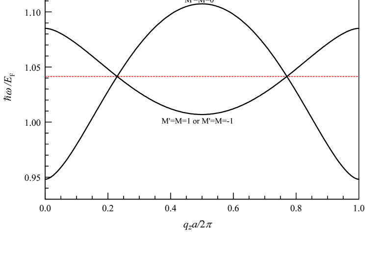
Figure 3: Plasmon dispersion relation in the first Brillouin zone for a periodic array of S2DEGs along the $z$ axis with period $a=3R$. The radius of each sphere is $R=10$ nm and $l_{F}=10$ is the angular momentum quantum number for the highest occupied electron state on each sphere. The horizontal solid line corresponds to the plasmon energy for the single shell with $L=1$.

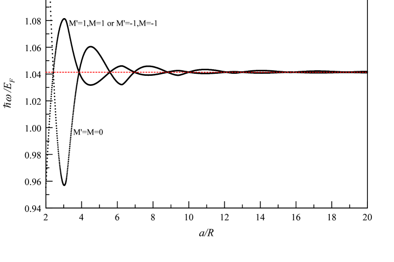
Figure 4: Plasmon variation for fixed $q_{z}R=2$ as a function of the separation $a$ of the shells along the $z$ axis.The horizontal dotted line gives the single shell plasmon energy for $L=1$.

Figure 5: Coulomb interaction matrix elements for a linear array of shells along the $x$ axis for the case when $L=L^{\prime}=1$ and $M,M^{\prime}=0,\pm 1$. The radius of each sphere is $R=10$ nm.

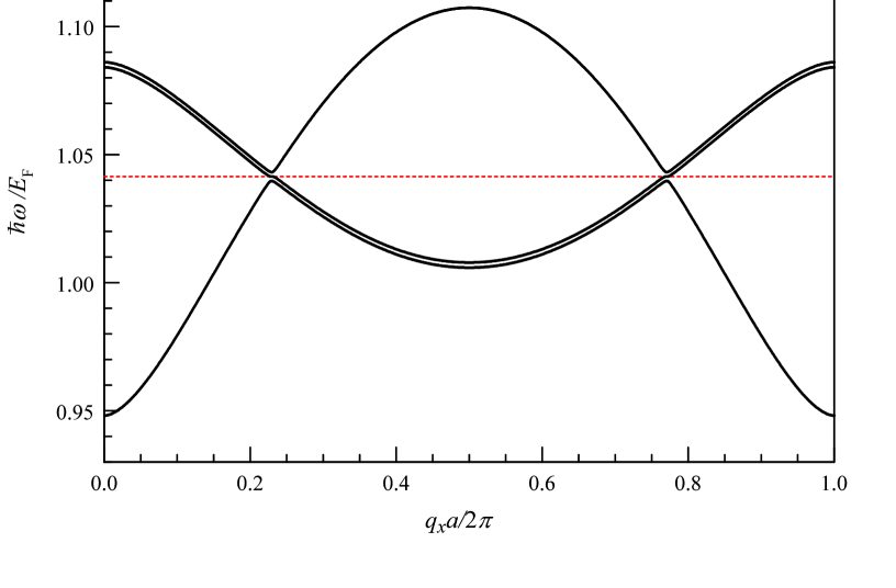
Figure 6: Plasmon dispersion relation for a linear array of spherical shells of radius $R=10$ nm separated by a distance $a=3R$ along the $x$ axis.

Figure 7: Anticrossing of the plasmon modes of Fig. 6 in the vicinity of the points (a) $q_{x}/2\pi a=0.23$ and (b) $q_{x}/2\pi a=0.77$.

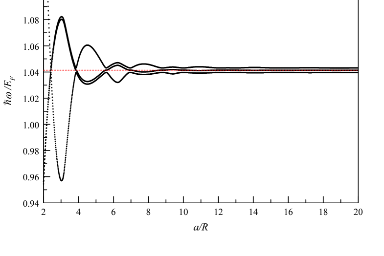
Figure 8: Variation of the plasmon excitation energies with separation between adjacent S2DEGs on a linear chain on the $x$ axis for chosen $q_{x}R=2$. The horizontal dashed line corresponds to the plasmon mode frequency for a S2DEG in isolation.

- (1) E. Osawa, Kagaku (Kyoto) 25, 854 (1970) [in Japanese].
- (2) J. F. Anacleto and M. A. Quilliam, Anal. Chem. 65, 2236 (1993).
- (3) H. W. Kroto, J. R. Heath, S. C. O’Brien, R. F. Curl and R. E. Smalley, Nat. 318, 162 (1985).
- (4) S. Iijima, J. Crystal Growth 50, 675 (1980).
- (5) P. R. Buseck, S. J. Tsipursky and R. Hettich, Sci. 257, 215 (1992).
- (6) J. Cami, J. Bernard-Salas, E. Peeters and S. E.Malek, Sci. 329, 180 (2010).
- (7) C. A. Poland, R. Duffin, I. Kinloch, A. Maynard, W. A. H. Wallace, A. Seaton, V. Stone, S. Brown, W. MacNee and K. Donaldson, Nat. Nanotechn. 3, 423 (2008).
- (8) Plinio Innocenzi and Giovanna Brusatin, Chem. Mater., 13, 3126 (2001).
- (9) L. Henrard,* F. Malengreau, P. Rudolf, K. Hevesi, R. Caudano, and Ph. Lambin, Th. Cabioc h, Phys. Rev. B59, 5832 (1999).
- (10) D. Östling, P. Apell and A. Rosen, Europhys. Lett. 21, 539 (1993).
- (11) G. Gensterblum, J. J. Pireaux, R. Gaudano, J. P. Vigneron, A. A. Lucas and W. Krätschmer, Phys. Rev. Lett. 67, 2171 (1991).
- (12) E. Schmen, J. Fink and W. Krätschmer, Europhys. Lett., 17, 51 (1992).
- (13) Lang Wei, Jiannian Yao, and Hongbing Fu, ACS Nano, 7 (9), pp 7573 7582 (2013).
- (14) Manish Chhowalla and Gehan A. J. Amaratunga, Nature 407, 164 (2000).
- (15) Takeshi Inaoka, Surface Science 273, 191 (1992).
- (16) J. Tempere, I. F. Silvera, and J. T. Devreese, Phys. Rev. B65, 195418 (2002).
- (17) Constantine Yannouleas, Eduard N. Bogachek, and Uzi Landman, Phys. Rev. B53, 10225 (1996).
- (18) D. Huang and G. Gumbs, Phys. Rev. B 46, 4147 (1992).
- (19) Godfrey Gumbs and G. R. Aǐzin, Physical Review B 65, 195407 (2002).
- (20) A. A. Lucas, L. Henrard, and Ph. Lambin, Phys. Rev. B 49, 2888 (1994).
- (21) Yang, Shu-Chun and Kobori, Hiromu and He, Chieh-Lun and Lin, Meng-Hsien and Chen, Hung-Ying and Li, Cuncheng and Kanehara, Masayuki and Teranishi, Toshiharu and Gwo, Shangjr, Nano Letters, 10, 2 (2010).
- (22) Nordlander, P. and Oubre, C. and Prodan, E. and Li, K. and Stockman, M. I., Nano Letters, 4, 5 (2004).
- (23) Godfrey Gumbs, Andrii Iurov, Antonios Balassis, and Danhong Huang, Journal of Physics: Condensed Matter 26, 135601 (2014).
- (24) M. S. Dresselhaus, G. Dresselhaus, P. C. Eklund,, Science of Fullerenes and Carbon Nanotubes: Their Properties and Applications, (Academic Press, 1995).
- (25) Li-Feng Wang and Quan-Shui Zheng, Appl. Phys. Lett. 90, 153113 (2007).
- (26) C. W. Chiu, F. L. Shyu, M. F. Lin, Godfrey Gumbs, and Oleksiy Roslyak, J. Phys. Soc. Jpn. 81, 104703 (2012).
- (27) Michael K. Yakes, Daniel Gunlycke, Joseph L. Tedesco, PaulM. Campbell, Rachael L.Myers-Ward, Charles R. Eddy, Jr., D. Kurt Gaskill, Paul E. Sheehan, and Arnaldo R. Laracuente, Nano Lett. 10, 15591562 (2010).
- (28) Nengjiu Ju, Aurel Bulgac, and John W. Phys. Rev. B 48, 9071, (1993).
- (29) R Singhal, D C Agarwal, Y K Mishra, F Singh, J C Pivin, R. Chandra and D K Avasthi, J. Phys. D: Appl. Phys. 42 155103 (2009).