New general approach in few-body scattering calculations:
Solving discretized Faddeev equations on a graphics processing unit

Abstract

Background:

The numerical solution of few-body scattering problems with realistic interactions is a difficult problem that normally must be solved on powerful supercomputers, taking a lot of computer time. This strongly limits the possibility of accurate treatments for many important few-particle problems in different branches of quantum physics.

Purpose:

To develop a new general highly effective approach for the practical solution of few-body scattering equations that can be implemented on a graphics processing unit.

Methods:

The general approach is realized in three steps: (i) the reformulation of the scattering equations using a convenient analytical form for the channel resolvent operator; (ii) a complete few-body continuum discretization and projection of all operators and wave functions onto a $L_{2}$ basis constructed from stationary wave packets and (iii) the ultra-fast solution of the resulting matrix equations using graphics processor.

Results:

The whole approach is illustrated by a calculation of the neutron-deuteron elastic scattering cross section below and above the three-body breakup threshold with a realistic $NN$ potential which is performed on a standard PC using a graphics processor with an extremely short runtime.

Conclusions:

The general technique proposed in this paper opens a new way for a fast practical solution of quantum few-body scattering problems both in non-relativistic and relativistic formulations in hadronic, nuclear and atomic physics.

I Introduction.

It is well known that a sharp contrast exists today in the quantum-mechanical treatment of few- and many-body systems between very effective and fast bound-state calculations, on the one hand, and very time-consuming few-particle scattering calculations on the other hand. Practical solutions for a discrete spectrum may incorporate many hundreds or even thousands particles with simple Coulomb-like interactions in atomic or molecular physics, or up to 20-25 nucleons with complicated realistic $NN$ interactions in nuclear physics, while even the solution of the four-nucleon scattering problem with realistic $NN$-interactions, especially above the three-body breakup threshold, represent a strong challenge for modern theorists Lazauskas_rep . There are at least two reasons for such a strong contrast. First, the few-body scattering problem includes complicated boundary conditions, especially above the three- or four-body breakup thresholds, and second, the multi-particle Hamiltonian has a degenerate continuous spectrum, so that each pair or triple of particles can be in infinite number of states at the same energy.

The first problem has been solved mathematically by formulation of the Faddeev–Yakubovsky equations whose full solution satisfies, as has been strictly proved Faddeev , all of the necessary boundary conditions. However, the price for this correct formulation is a very sophisticated form of these integral equations, whose kernels have complicated moving singularities. Therefore, in the previous four decades a lot of exact and approximate methods for solving the Faddeev–Yakubovsky equations were proposed. However, due to the complexity of realistic few-body scattering problems, practical solutions usually require a massively parallel implementation, so that even now exact Faddeev-like scattering calculations are performed mainly on powerful supercomputers (see e.g. the recent $3N$-calculations gloeckle12 ). The complexity of the few-body equations leads to the fact that an accurate numerical treatment for realistic few-body scattering problems remains available only to a limited number of experts.

The most effective way to treat the second key problem related to degeneracy of few-body continuous spectra of the total and channel Hamiltonians is their discretization by one or another method and usage of $L_{2}$ normalized states as approximations for exact continuum states. Nowadays, many such discretization methods exist (see, for example, a recent comprehensive review Lazauskas_rep ). However, it is still not clear whether these particular discretization methods give a discrete form of scattering equations, which permit a high degree of parallelism in a numerical solution. The last point is crucially important for further progress in few-body scattering calculations because even powerful supercomputers can not give essential acceleration of the calculations if the solution method does not permit an effective parallelization for all parts of the algorithm.

Quite recently, a new computational technique has been introduced based on the general-purpose graphics processing unit (GPGPU). This technique utilizes a graphics processing unit (GPU) which has been initially designed to carry out computations for computer graphics. Nowadays, GPUs are specialized to perform ultra-fast general purpose computations and they can replace a supercomputer realization in many particular cases. Also, special extensions of standard programming languages are developed to use GPU facilities in tedious scientific calculations (see e.g. CUDA ).

This technique has been actively pursued and successfully used in quantum chemistry CUDA_ch , in lattice QCD calculations CUDA_QCD , Monte-Carlo simulations etc. Recently, ab-initio nuclear structure GPU-calculations Vary have been performed as well as GPU treatments of Faddeev equations for quantum trimer systems yarevsky . It is of great interest to apply such GPU-techniques to realistic few-body scattering calculations. This would open new possibilities for accurate few-body studies in general and could make them more accessible to a wider number of researchers. However, the GPU realization requires an appropriate and specific formulation for scattering problems because this realization is most effective for the algorithms with a high degree of parallelism and minimal interdependence between data processing in parallel threads.

The present authors suggested in previous years the wave-packet continuum discretization technique nd1 ; nd2 which has been tested carefully for the model $NN$ interactions and found to be very efficient. One of the important features of the above discrete approach is that the resulting discretized form of the scattering equations is well suited for such a parallel realization. Below we show that such a massively parallel implementation of the whole solution can be made on a standard PC with a modern graphics processor that can perform all of the calculations using many thousands of parallel threads.

In the present paper we have also made a generalization of the wave-packet approach to few-body equations with fully realistic $NN$ interaction which is not a trivial problem and requires a new determination for the multi-channel resolvent in an analytical form. So we included a section with this description in the present paper .

The paper is organized as follows. In Sect. II we summarize the main features of the WP approach and describe how it is used to solve three-body scattering problem. In Sect. III the case of the coupled-channel two-body input interaction is discussed and formulas for the three-body channel resolvent are given. The results for the $nd$ elastic scattering problem are represented in Sect. IV. Section V is dedicated to a description of our first GPU tests for the problem in question and a comparison of the corresponding computational efficiency of the CPU and GPU realizations on the same PC. The main results of the paper are summarized in the conclusion.

II New general approach in few-body scattering calculations.

The present work discusses the solution few- and many-body scattering problems in atomic, molecular, nuclear and hadronic physics. Here we discuss in detail all of the steps needed to implement our new approach and we illustrate the whole technique using a non-trivial example — the solution of the Faddeev equations for $n-d$ scattering below and above the three-body breakup threshold with a realistic $NN$ interaction.

II.1 The basic features of the approach

In our approach, we change all of the steps used in the conventional procedure for solving the Faddeev equations in momentum space.

(i) The first step is to replace the conventional form of the Faddeev integral equation, e.g. for a transition operator $U$ describing elastic $nd$ scattering gloeckle ,

$$U=PG_{0}^{-1}+Pt_{1}G_{0}U,$$ (1)

with the half-shell equivalent form

$$U=Pv_{1}+Pv_{1}G_{1}U.$$ (2)

Here $v_{1}$ is the two-body interaction, $t_{1}$ is the two-body $t$-matrix, $G_{0}$ is the resolvent of the free three-body Hamiltonian, $H_{0}$, $P=P_{12}P_{23}+P_{13}P_{23}$ is the particle permutation operator and $G_{1}=[E+i0-H_{1}]^{-1}$ is the resolvent of the channel Hamiltonian

$$H_{1}=h_{1}\oplus h_{0}^{1},$$ (3)

where $h_{1}=h_{0}+v_{1}$ is the two-body $NN$ sub-Hamiltonian and $h_{0}^{1}$ is sub-Hamiltonian describing free motion of the third nucleon relative to the $NN$ subsystem. The index $1$ is the Jacobi-set index of the initial state.

One of the main purposes for such a replacement is to change the required two-body input: instead of fully off-shell two-body $t$-matrices at many energies, we suggest employing two-body interactions $v_{1}$ in combination with the channel resolvent $G_{1}$. However, in such a replacement, one has to evaluate additionally the channel resolvent operator $G_{1}$. Fortunately, in the wave-packet approach, the finite-dimensional approximation for this operator is calculated easily in a closed analytical form nd1 .

Moreover, the whole energy dependence appears now in the channel resolvent operator (rather than in the off-shell $t$-matrix, as in the conventional formulation), which is calculated explicitly. So that, with such a replacement, we can find a solution of few-body scattering equations at many energies almost with the same computational effort that is needed for a single energy.

Another important advantage of our approach is a new treatment of three-body breakup. Contrary to the conventional approach, we treat three- or many-body breakup processes as particular cases of inelastic excitations (into states of the discretized continuum) nd2 . Such a treatment strongly facilitates breakup calculations.

(ii) The second step is to project the integral kernels of the reformulated Faddeev equations and the solution onto a special orthogonal basis of the stationary wave packets (WPs), which corresponds to a formulation of the scattering problem on a momentum lattice. Such basis is very appropriate for constructing normalized analogs of continuum states for the channel Hamiltonian $H_{1}$. It follows that the solution of the three-body scattering problem is described in the terms of asymptotic channel states, in contrast to conventional approach which employs free three-body states (the plane waves).

Such a projection of the three-body scattering equations onto a three-body WP basis results in matrix equations which allow us to circumvent the main difficulties that arise in the conventional solution of the initial singular integral equation. Firstly, the use of a finite matrix for the permutation operator in a discrete WP basis eliminates the need for the very numerous multi-dimensional interpolations of a given solution into the “rotated” Jacobi set during iterations. Further, all singularities of the Faddeev kernel (in the form $Pv_{1}G_{1}$) are isolated now in the channel resolvent $G_{1}$ and thus can be easily smoothed and averaged when using the WP representation nd1 . At last, the resulting matrix equations can be solved directly at real energies without any contour rotations or deformations onto complex plane, which are often employed in the solution of singular integral equations.

The resulting matrix equation (of high dimension) obtained in the WP approach is solved by simple iterations when they converge or otherwise by applying an additional Pade-approximant summation. The computational scheme turns out to be very efficient and thus the whole calculation can be performed even on a standard PC.

Following these steps, in our previous papers, nd1 ; nd2 , we studied elastic scattering and breakup cross sections in a $3N$ system with a central $NN$ potential. But it was still unclear if the advantages of the above computational scheme remain valid for realistic $NN$ interactions including tensor, spin-orbit etc. components and in the particularly when the number of contributing spin-orbital partial channels is large. To investigate this question we will apply our approach to a three-nucleon system interacting with a realistic $NN$ interaction, including a tensor component (the Nijmegen $NN$ potential nijm ), at energies below and above three-body breakup threshold.

(iii) To further extend the complexity of scattering problems that can be treated accurately, it is desirable to develop a highly parallel algorithm for the solution of the resulting matrix equations of large dimension. The third step is to parallelize the algorithm to adapt it for computations by a GPU. Such a GPU realization is shown in the present paper to make the solution of resulting matrix equations (derived from multi-channel system of integral Faddeev equations) extremely fast even on a standard PC.

II.2 Discrete form of the Faddeev equation in wave-packet representation.

Here we briefly describe our approach based on a continuum discretization using the stationary wave packets. We illustrate this using the example of the Faddeev equation (2) for the transition operator $U$ for $nd$ scattering (further details see in nd1 ; nd2 ).

II.2.1 Definition of momentum lattice basis functions

To construct the three-body WP basis functions, we start from the two-body case and introduce partitions of the continua of two free sub-Hamiltonians, $h_{0}$ and $h_{0}^{1}$, onto non-overlapping intervals $\{\mathfrak{D}_{i}\equiv[\epsilon_{i-1},\epsilon_{i}]\}_{i=1}^{M}$ and $\{\bar{\mathfrak{D}}_{j}\equiv[{\cal E}_{j-1},{\cal E}_{j}]\}_{j=1}^{N}$ respectively. These sub-Hamiltonians describe the free motion of particles 2 and 3 with relative momentum $p$ and the free motion of particle 1 with momentum $q$ relative to the center of mass of the pair (23), respectively. Thus the free stationary wave packets $|\mathfrak{p}_{i}\rangle$ and $|\mathfrak{q}_{j}\rangle$ are built as integrals of free solutions $|p\rangle$ and $|q\rangle$ over the discretization bins:

$$|\mathfrak{p}_{i}\rangle=\frac{1}{\sqrt{B_{i}}}\int_{\mathfrak{D}_{i}}f(p)|p\rangle dp,\ |\mathfrak{q}_{j}\rangle=\frac{1}{\sqrt{\bar{B}_{j}}}\int_{\bar{\mathfrak{D}}_{j}}\bar{f}(q)|q\rangle dq,$$ (4)

where $B_{i},\bar{B}_{j}$ and $f(p),\bar{f}(q)$ are normalization factors and weight functions respectively nd1 ; nd2 . Here and below we denote the functions and values corresponding to $q$-variable with additional bar mark to distinguish them from the functions corresponding to the $p$-variable.

When constructing the three-body WP basis one should take into account spin and angular parts of the basis functions. We use the following quantum numbers for the subsystems and the whole three-body system according to the $(jj)$-coupling scheme:

$$\alpha=\{l,s,j\};\qquad\beta=\{\lambda,I\};\qquad\Gamma=\{J,\pi,T\},$$ (5)

where $l,s$ and $j$ are $NN$ quantum numbers: $l$ is an orbital momentum, $s$ is a spin and ${\bf j}={\bf l}+{\bf s}$ is a total angular momentum of the subsystem (the interaction potential depends on the value of $j$). The other quantum numbers are the following: $\lambda$ is an orbital momentum and ${\bf I}=\mbox{\boldmath$\lambda$}+\mbox{\boldmath$\sigma$}$ is a total momentum of the third nucleon, where $\sigma={\frac{1}{2}}$ is its spin. Finally, ${\bf J}={\bf j}+{\bf I}$ is a total angular momentum of the three-body system, $T$ is the total isospin and $\pi$ is parity, all of them are conserved. Let’s also note that the pair isospin $t$ can be defined by values of $l$ and $s$, because the sum $l+s+t$ must be odd.

The free WP states should be defined for each partial wave $l$ and $\lambda$ and further they are multiplied by appropriate spin-angular states. Thus the three-body basis function can be written as:

$$|X_{ij}^{\Gamma\alpha\beta}\rangle=|\mathfrak{p}_{i}^{l}\rangle\otimes|\mathfrak{q}_{j}^{\lambda}\rangle|\alpha,\beta:\Gamma\rangle,$$ (6)

where $|\alpha\rangle$ is a spin-angular state of the $NN$ pair, $|\beta\rangle$ is a spin-angular state of the third nucleon, and $|\Gamma\rangle$ is a set of three-body quantum numbers.

The state (6) is the WP analog of the exact plane wave state in three-body continuum $|p,q;\alpha,\beta:\Gamma\rangle$ for the three-body free Hamiltonian $H_{0}=h_{0}\oplus h_{0}^{1}$.

The free stationary wave packets defined in eq. (4) with unit weights are step-like functions in the momentum representation nd1 ; nd2 while the three-body free WP basis functions are constant inside the cells of the lattice built by a convolution of two one-dimensional cells $\{\mathfrak{D}_{i}\}_{i=1}^{M}$ and $\{\bar{\mathfrak{D}}_{j}\}_{j=1}^{N}$. We refer to the free WP basis as a lattice basis. We denote the two-dimensional bins (i.e. the lattice cells) by $\mathfrak{D}_{ij}=\mathfrak{D}_{i}\otimes\bar{\mathfrak{D}}_{j}$.

II.2.2 The wave-packet basis for the channel Hamiltonian

In the case of a single-channel two-body input interaction (e.g. the central one), we have demonstrated nd1 ; nd2 that it is possible to define scattering WPs corresponding to the exact scattering wave functions $|\psi_{p}\rangle$ of the sub-Hamiltonian $h_{1}$:

$$|z_{k}\rangle=\frac{1}{\sqrt{C_{i}}}\int_{{\Delta}_{i}}w(p)|\psi_{p}\rangle dp,$$ (7)

where $\Delta_{i}$ are partition intervals and $C_{i}$ and $w(p)$ are a normalization factor and a weight function.

To use the states (7) practically, one can approximate them with the pseudostates of the sub-Hamiltonian $h_{1}$ in some $L_{2}$ basis nd1 ; nd2 . Also it has been shown that the free WP basis is very appropriate to approximate scattering states because the respective functions have a very long-range behavior in configuration space. So we can calculate the eigenstates (the bound and pseudostates) of the sub-Hamiltonian $h_{1}$ matrix in the two-body WP-basis $\{|\mathfrak{p}_{i}\rangle\}_{i=1}^{M}$ via a diagonalization procedure. As a result one gets the eigenstates of the $h_{1}$ sub-Hamiltonian expanded in the free WP basis (for each partial wave $l$):

$$|z_{k}^{l}\rangle\approx\sum_{i=1}^{M}O_{ki}^{l}|\mathfrak{p}_{i}^{l}\rangle.$$ (8)

For the case of a central interaction, the three-body quantum numbers for the channel Hamiltonian $H_{1}$ are the same as those for the three-body free Hamiltonian $H_{0}$, so that total three-body WP states corresponding to the channel Hamiltonian $H_{1}$ (three-body scattering wave packets — SWP) are built as direct products of the two-body WPs with the same spin-angular quantum numbers $\alpha,\beta,\Gamma$:

$$|Z_{kj}^{\Gamma\alpha\beta}\rangle\equiv|z_{k}^{l}\rangle\otimes|\mathfrak{q}_{j}^{\lambda}\rangle|\alpha,\beta:\Gamma\rangle.$$ (9)

The main advantage of the basis constructed from SWP (9) is that one gets an explicit analytical and even diagonal form for the matrix of three-body channel resolvent $G_{1}$ nd1 ; nd2 .

Having the WP basis for the channel-Hamiltonian (9) at our disposal, it is possible to project all of the constituents of the integral equation (2) and find its finite-dimensional, i.e. matrix, analog. As an important result of the projecting of the channel operator $G_{1}v_{1}$ onto the SWP-basis, one gets the main part of the Faddeev kernel matrix in a convenient analytical form, with a completely analytical energy dependence, in sharp contrast to a conventional approach with a fully off-shell $t$-matrix in a numerical form.

II.2.3 The matrix of the permutation operator

The permutation operator matrix $\mathbb{P}$ in the three-body SWP basis $|Z_{kj}^{\Gamma\alpha\beta}\rangle$ can be expressed through the overlap matrix ${\mathbb{P}}^{0}$ in the free WP basis $|X_{ij}^{\Gamma\alpha\beta}\rangle$ using the rotation matrices $\mathbb{O}$ from the expansion (8) :

$$\langle Z_{kj}^{\Gamma\alpha\beta}|P|Z_{k^{\prime}j^{\prime}}^{\Gamma\alpha^{\prime}\beta^{\prime}}\rangle\approx\sum_{ii^{\prime}}O_{ki}^{l}O_{k^{\prime}i^{\prime}}^{l^{\prime}*}\langle X_{ij}^{\Gamma\alpha\beta}|P|X_{i^{\prime}j^{\prime}}^{\Gamma\alpha^{\prime}\beta^{\prime}}\rangle.$$ (10)

A matrix element of the operator $P$ in the free WP basis is equal to the overlap between basis functions defined in different Jacobi sets. Such a matrix element can be calculated by integration with the basis functions over the momentum lattice cells:

$$\langle X_{ij}^{\Gamma\alpha\beta}|P|X_{i^{\prime}j^{\prime}}^{\Gamma\alpha^{\prime}\beta^{\prime}}\rangle=\int_{\mathfrak{D}_{ij}}p^{2}dpq^{2}dq\int_{\mathfrak{D}^{\prime}_{i^{\prime}j^{\prime}}}(p^{\prime})^{2}dp^{\prime}(q^{\prime})^{2}dq^{\prime}\times$$

$$\frac{f^{*}(p)\bar{f}^{*}(q)f(p^{\prime})\bar{f}(q^{\prime})}{\sqrt{B_{i}B_{i^{\prime}}\bar{B}_{j}\bar{B}_{j^{\prime}}}}\langle pq,\alpha\beta:\Gamma|P|p^{\prime}q^{\prime},\alpha^{\prime}\beta^{\prime}:\Gamma\rangle,\qquad\qquad$$ (11)

where the prime on the lattice cell $\mathfrak{D}^{\prime}_{i^{\prime}j^{\prime}}$ indicates that the cell belongs to the other Jacobi set while $\langle pq,\alpha\beta:\Gamma|P|p^{\prime}q^{\prime},\alpha^{\prime}\beta^{\prime}:\Gamma\rangle$ is the kernel of particle permutation operator in momentum space. This kernel, as is well known gloeckle , is proportional to the product of a Dirac delta and a Heaviside theta function. However, due to integration in the eq. (11), these singularities get averaged over the momentum lattice cells and, as a result, the elements of the permutation operator matrix in the WP basis are finite and regular.

The matrix element in the eq. (11) can be calculated using a double numerical integration. The practical technique of such calculation is described in the Appendix to the present paper.

II.2.4 Matrix analog of the Faddeev equation for elastic $nd$ scattering and breakup

Having evaluated the matrix of permutation operator $P$, the calculation of the kernel $Pv_{1}G_{1}$ matrix becomes fast and straightforward.

As a result of projecting the integral equation (2) onto the three-body SWP basis, one gets its matrix analog (for the each set of three-body quantum numbers $\Gamma$):

$${\mathbb{U}}={\mathbb{P}}{\mathbb{V}}_{1}+{\mathbb{P}}{\mathbb{V}}_{1}{\mathbb{G}}_{1}{\mathbb{U}}.$$ (12)

Here ${\mathbb{P}}$, ${\mathbb{V}}_{1}$ and ${\mathbb{G}}_{1}$ are matrices of the permutation operator, the pair interaction and the channel resolvent respectively defined in the SWP basis.

The on-shell elastic amplitude for the $nd$ scattering in the WP representation is defined by a diagonal matrix element of the $\mathbb{U}$-matrix nd1 ; nd2 :

$$A_{\rm el}^{\Gamma\alpha_{0}\beta}(q_{0})\approx\frac{2m}{3q_{0}}\frac{\langle Z^{\Gamma\alpha_{0}\beta}_{0j_{0}}|\mathbb{U}|Z^{\Gamma\alpha_{0}\beta}_{0j_{0}}\rangle}{\bar{d}_{j_{0}}},$$ (13)

where $m$ is the nucleon mass, $q_{0}$ is the initial two-body momentum and $|Z^{\Gamma\alpha_{0}\beta}_{0j_{0}}\rangle=|z_{0}^{\alpha_{0}},{\mathfrak{q}}_{j_{0}}^{\lambda};\alpha_{0},\beta:\Gamma\rangle$ is the SWP basis state corresponding to the initial scattering state. Here $|z_{0}^{\alpha_{0}}\rangle$ is the bound state of the pair (the deuteron, in our case), the index $j_{0}$ denotes the bin $\bar{\mathfrak{D}}_{j_{0}}$, including the on-shell momentum $q_{0}$, and $\bar{d}_{j_{0}}$ is the momentum width of this bin.

It should be noted here that in our discrete WP approach the three-body breakup is treated as a particular case of an inelastic scattering nd2 (defined by the transitions to the specific two-body discretized continuum states), so that the breakup amplitude can be defined in terms of the same matrix $\mathbb{U}$ determined from eq. (12).

For the case of the tensor components of the $NN$ interaction (or other coupled-channel two-body interactions $v_{1}$), the generalization of the whole formalism is straightforward. However, it is necessary to take into account some new aspects related to the discretized spectrum of the two-body multichannel Hamiltonian $h_{1}$ to build the correct approximation for the discretized resolvent $G_{1}$.

III Channel resolvent in case of a coupled-channel interaction.

III.1 Construction of SWP basis for a coupled-channel sub-Hamiltonian

The three-body SWP states corresponding to the channel Hamiltonian $H_{1}$ can be defined similarly to the one-channel two-body interaction case, i.e. as direct products of two-body WP states for the $h_{0}^{1}$ and $h_{1}$ sub-Hamiltonians (jointly with the bound-state) multiplied by spin-angular functions of the system. However, here the possible spin-angular couplings in the $\{23\}$ subsystem due to the tensor component in a pairwise interaction $v_{1}$ should be taken into account.

Recently, the present authors have developed a convenient approach for solving multichannel scattering problems via a straightforward diagonalization of the multichannel Hamiltonian in a WP basis — the discrete spectral-shift (DSS) formalism KPRF . In this approach, the multichannel Hamiltonian pseudostates have been shown to correspond to scattering wave functions defined in the so called eigenchannel representation (ER) greiner for which the multichannel $S$-matrix is diagonal.

Let’s introduce two types of scattering states of the sub-Hamiltonian $h_{1}$: the scattering states $|\psi_{p}^{l}\rangle$ (which include radial and orbital parts) corresponding to the initial wave with a definite orbital momentum $l$ and the scattering states defined in the ER $|\psi^{\varkappa}_{p}\rangle$, where $\varkappa$ is an eigenchannel index. In case of a tensor $NN$ interaction, the scattering states $|\psi^{\varkappa}_{p}\rangle$ are linear combinations of states $|\psi_{p}^{l}\rangle$, e.g. the coupled pairs ${}^{3}S_{1}-{}^{3}D_{1}$, ${}^{3}P_{2}-{}^{3}F_{2}$ etc.

The main advantage of the ER formalism is that one gets the following spectral expansion for the resolvent of the pair sub-Hamiltonian $g_{1}(E)\equiv[E+i0-h_{1}]^{-1}$ (see e.g. KPR_Yaf14 ):

$$g_{1}(E)=\frac{|z_{0}\rangle\langle z_{0}|}{E-\epsilon_{0}}+\sum_{\varkappa}\int_{0}^{\infty}\frac{|\psi^{\varkappa}_{p}\rangle\langle\psi^{\varkappa}_{p}|}{E+i0-\frac{p^{2}}{m}}dp,$$ (14)

which is diagonal in the eigenchannel index $\varkappa$. In eq. (14), $\epsilon_{0}$ is an energy of the bound state $|z_{0}\rangle$ and $m$ is the nucleon mass.

Thus, it is convenient to construct multi-channel two-body SWP’s as integrals of exact scattering wave functions of the sub-Hamiltonian $h_{1}$ defined in the ER:

$$|z_{\varkappa,i}\rangle=\frac{1}{\sqrt{C_{i}^{\varkappa}}}\int_{\Delta_{i}^{\varkappa}}w(p)|{\psi}_{p}^{\varkappa}\rangle dp,\quad i=1,\ldots,M^{\varkappa},$$ (15)

where $\Delta_{i}^{\varkappa}\equiv[E_{i-1}^{\varkappa},E_{i}^{\varkappa}]$ are new partition intervals whose parameters might be different for different $\varkappa$.

The crucial feature of the DSS formalism defined in KPRF is that these multichannel SWP can be constructed (jointly with the deuteron bound state wave function) as pseudostates of the Hamiltonian $h_{1}$ matrix in the multichannel free WP basis $|{\mathfrak{p}}_{i}^{l}\rangle$ (where radial and angular parts of wave functions included). Because $l$ is not conserved, for each value of total momentum $j$, the two-channel $h_{1}$ sub-Hamiltonian states are constructed from free WP bases $\{|{\mathfrak{p}}_{i}^{l}\rangle\}_{l=l_{1},l_{2}}$ defined for both possible values of $l_{1}$ and $l_{2}$.

Finally, we have at our disposal the multichannel SWP basis functions which are related to the free WPs by a simple orthogonal transformation as in the one-channel case (8):

$$|z_{\varkappa_{\tilde{\alpha}},k},{\tilde{\alpha}}\rangle=\sum_{i=1}^{M}\sum_{l}O_{ki}^{\varkappa_{\tilde{\alpha}}l}|\mathfrak{p}_{i}^{l},\alpha\rangle,$$ (16)

where the spin-angular parts of wave functions are taken into account as well and the multi-index ${\tilde{\alpha}}=\{\varkappa_{\tilde{\alpha}},s,j\}$ related to the ER is introduced. Below we will not detail the index $\varkappa_{\tilde{\alpha}}$ which is a part of the multi-index ${\tilde{\alpha}}$.

In this way, we construct the three-body SWP basis functions for the channel Hamiltonian $H_{1}$ as direct products of the two-body ones for the $h_{0}^{1}$ and $h_{1}$ sub-Hamiltonians:

$$|Z^{\Gamma{\tilde{\alpha}}\beta}_{kj}\rangle\equiv|z_{\varkappa_{\tilde{\alpha}},k}^{{\tilde{\alpha}}}\rangle\otimes|\mathfrak{q}_{j}^{\beta}\rangle|{\tilde{\alpha}},\beta:\Gamma\rangle.$$ (17)

These states are WP analogs of the three-body ER scattering states $|\psi^{\varkappa_{\tilde{\alpha}}}_{p},q;{\tilde{\alpha}},\beta:\Gamma\rangle$ of the channel Hamiltonian $H_{1}$.

Hence, starting from free WP bases for each two-body sub-Hamiltonian one gets a set of basis states both for the three-body free and channel Hamiltonians, $H_{0}$ and $H_{1}$ respectively, which are related to each other by a simple matrix rotation.

III.2 Resolvent of the channel Hamiltonian

The spectral expansion of the three-body channel resolvent $G_{1}$ in the ER can be found straightforwardly by making a convolution of the multi-channel subresolvent $g_{1}$ with the resolvent $g_{1}^{0}(E)=[E+i0-h_{0}^{1}]^{-1}$ for the free sub-Hamiltonian $h_{0}^{1}$ of the third nucleon

$$G_{1}(E)=\frac{1}{2{\pi\rm i}}\int_{-\infty}^{\infty}{\rm d}\varepsilon g_{1}(\varepsilon)g_{0}^{1}(E-\varepsilon).$$ (18)

This leads to the following representation for the multi-channel three-body resolvent operator $G_{1}$ via the scattering eigenfunctions of the $NN$ subsystem defined in the ER:

$$G_{1}(E)=\sum_{\Gamma,{\tilde{\alpha}}_{0},\beta}\int_{0}^{\infty}{\rm d}q\frac{|z_{0},q,{\tilde{\alpha}}_{0}\beta:\Gamma\rangle\langle z_{0},q,{\tilde{\alpha}}_{0}\beta:\Gamma|}{E+{\rm i}0-\epsilon_{0}-\frac{3q^{2}}{4m}}+$$

$$\sum_{\Gamma,{\tilde{\alpha}},\beta}\int_{0}^{\infty}{\rm d}p{\rm d}q\frac{|\psi^{\varkappa_{\tilde{\alpha}}}_{p},q;{\tilde{\alpha}},\beta:\Gamma\rangle\langle\psi^{\varkappa_{\tilde{\alpha}}}_{p},q;{\tilde{\alpha}},\beta:\Gamma|}{E+{\rm i}0-\frac{p^{2}}{m}-\frac{3q^{2}}{4m}}.$$ (19)

The first term (the bound-continuum part) in eq. (19) is a spectral sum over three-body states corresponding to the free motion of the third nucleon relative to the deuteron. The second term (the continuum-continuum part) in eq. (19) for the channel resolvent includes channel three-body states with $NN$ pair interacting in the continuum (in the ER) and its imaginary part is defined by a discontinuity across the three-body cut on the Riemann energy surface.

By projecting the channel resolvent operator onto the three-body SWP basis defined in eq. (17), one can find analytical formulas for matrix elements of operator $G_{1}$ in such a basis. The respective matrix is diagonal in all wave-packet and spin indices:

$$\langle Z_{kj}^{\Gamma{\tilde{\alpha}}\beta}|G_{1}(E)|Z^{\Gamma{\tilde{\alpha}}^{\prime}\beta^{\prime}}_{k^{\prime}j^{\prime}}\rangle=\delta_{kk^{\prime}}\delta_{jj^{\prime}}\delta_{{\tilde{\alpha}}{\tilde{\alpha}}^{\prime}}\delta_{\beta\beta^{\prime}}G^{\Gamma{\tilde{\alpha}}\beta}_{kj}(E).$$ (20)

Here the diagonal matrix elements $G^{\Gamma{\tilde{\alpha}}\beta}_{kj}(E)$ depend, in general, on the spectral partition parameters (i.e. $\Delta_{k}^{\varkappa_{\tilde{\alpha}}}$ and $\bar{D}_{j}$ values) and total energy $E$ only. These matrix elements do not depend explicitly on the interaction potential $v_{1}$.

The matrix elements $G^{\Gamma{\tilde{\alpha}}\beta}_{kj}(E)$ are defined as integrals over the respective momentum intervals for the bound-continuum part of the whole operator:

$$G^{\Gamma{\tilde{\alpha}}_{0}\beta}_{0j}(E)=\frac{1}{{\bar{B}}_{j}}\int_{\bar{\mathfrak{D}}_{j}}\frac{|\bar{f}(q)|^{2}{\rm d}q}{E+{\rm i}0-\epsilon_{n}^{\alpha}-\frac{3q^{2}}{4m}},$$

and for the continuum-continuum part:

$$G^{\Gamma{\tilde{\alpha}}\beta}_{kj}(E)=\frac{1}{C_{k}^{\varkappa_{\tilde{\alpha}}}\bar{B}_{j}}\int_{\Delta_{k}^{\varkappa_{\tilde{\alpha}}}}\int_{\bar{\mathfrak{D}}_{j}}\frac{|w(p)|^{2}|\bar{f}(q)|^{2}{\rm d}p{\rm d}q}{E+{\rm i}0-\frac{p^{2}}{m}-\frac{3q^{2}}{4m}}.$$

If the solution of the scattering equations in the finite-dimensional WP basis converges with increasing the basis dimension, the final result turns out to be independent of the particular spectral partition parameters.

Representations (20a) and (20b) for the channel resolvent are the basis of the wave-packet approach, since, after a straightforward analytical evaluation of the integrals in (20a) and (20b), one gets explicit formulas for the three-body resolvent and thus a drastic simplification of the solution of a general three-body scattering problem. These analytical expressions can be used directly to solve the matrix Faddeev equation in eq. (12).

IV Solution of the n-d scattering problem with a realistic $NN$ interaction

In this section the effectiveness of the new approach in few-body calculations will be illustrated by solving the Faddeev equations for $nd$ scattering with the realistic Nijmegen $NN$ potential nijm .

The $S$-matrix of elastic $Nd$ scattering is usually parameterized by the eigen phase shifts and mixing angles in the total channel spin $\mbox{\boldmath$\Sigma$}={\mathbf{s}}+\mbox{\boldmath$\sigma$}$ representation (here $s$ is the $NN$ pair spin and $\sigma$ is a spin of the third nucleon). Unitary transformation between amplitudes defined in the representation of the total angular momentum of the third nucleon $I$ and the $\Sigma$-representation is given by the matrix gloeckle :

$$U^{J}_{\lambda^{\prime}\Sigma^{\prime},\lambda\Sigma}=\sum_{I,I^{\prime}}\sqrt{\hat{I}^{\prime}\hat{\Sigma}^{\prime}}\,(-1)^{J-I^{\prime}}\left\{\begin{array}[]{ccc}\lambda^{\prime}&1/2&I^{\prime}\\ j&J&\Sigma^{\prime}\end{array}\right\}\times$$ (23)

$$\sqrt{\hat{I}\hat{\Sigma}}\,(-1)^{J-I}\left\{\begin{array}[]{ccc}\lambda&1/2&I\\ j&J&\Sigma\end{array}\right\}U^{J}_{\lambda^{\prime}I^{\prime},\lambda I}.$$ (26)

In the Figs. 1-3 the results of our fully discrete calculations for elastic $nd$ scattering with the Nijm I $NN$ interaction performed within the WP approach are compared with the results of conventional Faddeev calculations of the Bochum–Krakow group gloeckle .

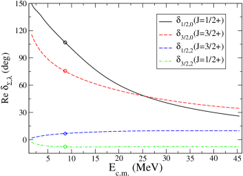
Figure 1: (Color online) Some of $S$- and $D$-wave partial phase shifts of the elastic $nd$ scattering obtained within the WP approach (solid lines) and within the standard Faddeev calculations (circles) gloeckle .

In the example, we restricted ourselves to the total isospin value $T=1/2$ and took into account all of the pairwise $NN$ channels with two-body total angular momentum $j\leq 3$ (this gives up to 54 spin-angular channels).

In Fig. 1 the results for the lowest even partial phase shifts $\delta^{J\pi}_{\Sigma\lambda}$ of elastic $nd$ scattering both below and above a three-body breakup threshold are shown. In the example, we employed WP bases with dimensions $M=N=144$ along two Jacobi coordinates. This gives a matrix system with the dimension $144\times 144=20736$ which has been handled easily on an ordinary PC in contrast to typical conventional calculations for similar Faddeev system which require supercomputer facilities (see e.g. gloeckle12 ). It should be especially emphasized that the calculation of the phase shifts at 100 different energy values displayed in Fig. 1 takes in our approach only about twice as much time as the calculation for a single energy because for all energies we employ the same permutation matrix $\mathbb{P}$ which is calculated only once.

In Fig. 2 our results for the differential cross section for elastic $nd$ scattering at 13 MeV are compared to the results of conventional Faddeev calculations gloeckle . While in Fig. 3 the same comparison is given for the neutron vector analyzing powers $A_{y}$ for the elastic $nd$ scattering at 35 MeV. Here the WP basis with dimension $M\times N=100\times 100$ has been used and the partial waves with the total angular momentum up to $J\leq 17/2$ have been taken into account.

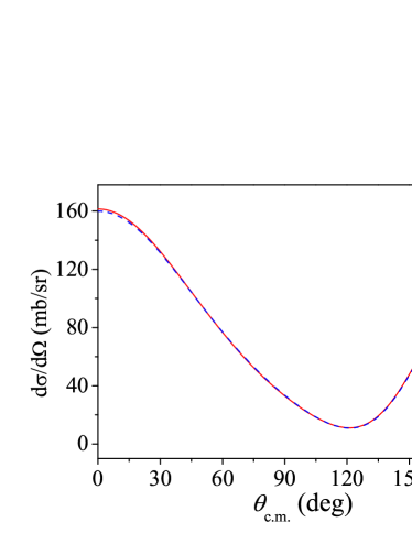
Figure 2: (Color online) The differential cross section for elastic $nd$ scattering at 13 MeV obtained via the WP technique (solid line) and within the standard Faddeev calculations gloeckle (dashed line).

It is clear from all of the above illustrative examples that one can achieve almost perfect agreement between our results and the results of the standard Faddeev calculations gloeckle performed on a powerful supercomputer.

The present calculations were performed on the serial PC with an Intel i7-3770K (3.50GHz) processor with 32 GB of RAM. The real CPU computational time (which includes the permutation matrix evaluation), i.e. the total calculation which starts from two-body interaction potential and ends with partial three-body amplitudes for a 54-channel calculation with the basis dimension $10^{4}$ for a single value of the total angular momentum $J$ and parity takes about 7 minutes.

Although the whole calculation for many partial waves will take a longer time, there is the possibility within the present approach to accelerate the whole calculation and thus solve more complicated scattering problems already using an ordinary PC. So, keeping in mind our general aim to simplify and accelerate drastically realistic many-body scattering calculations in nuclear, atomic, molecular etc. studies by using a discrete matrix reduction of the integral scattering equations in the WP scheme, we propose to employ the ultra-fast GPGPU technique to further optimize the solution of the resulting matrix equations.

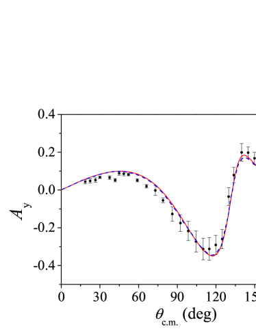
Figure 3: (Color online) The neutron vector analyzing power $A_{y}$ for the elastic $nd$ scattering at 35 MeV obtained within WP approach (solid line) compared to the result from gloeckle (dashed line) and the experimental $pd$ data pd_exp .

V Solution of the Faddeev matrix equation using GPU

In this section, we demonstrate a high efficiency of using a graphics processor in numerical solution of the above matrix equation for the three-body scattering problem.

V.1 Parallelization of a numerical algorithm.

First we describe the overall numerical scheme for solving the three-body scattering problem in the WP formalism, paying particular attention to those aspects that are important for an efficient parallelization.

The use of a fixed matrix for the permutation operator completely eliminates the necessity of the numerous and time consuming interpolations of a current solution in the iterations. These computations take the majority of the computing time in the standard integral approach. Contrary to this, in our approach, the main computational effort (in case of CPU-calculations) are spent on a calculation of the permutation matrix ${\mathbb{P}}^{0}$ in the lattice WP basis. However, the matrix ${\mathbb{P}}^{0}$ is independent of energy, and therefore, being calculated once, it can be used to solve the scattering problem at many energies, as well as for various two-particle input interactions. While in the standard approach, the whole calculation must be repeated for each energy and for each type of two-body interaction.

The main difficulty which is met in the practical solution of the matrix equation (12) is its large dimension. So, it is impossible even to store the entire matrix of the kernel $\mathbb{K}={\mathbb{P}}{\mathbb{V}}_{1}{\mathbb{G}}_{1}$ in a RAM of a computer. However, one can effectively employ the fact that the matrix $\mathbb{K}$ can be represented as a product of four matrices: a very sparse matrix ${\mathbb{P}}^{0}$ (only about 1 % of its matrix elements are nonzero nd2 ), a diagonal matrix $G_{1}$ and two block matrices. So that, it is sufficient to store only factors of the matrix $\mathbb{K}$ instead of all its matrix elements ( only the nonzero elements of the sparse matrix are stored). In this way, the required memory can be reduced by about 100 times. This eliminates the need for an external memory in the process of iteration, which in turn reduces a computational time by an order of magnitude even for a conventional CPU realization.

So, our overall numerical scheme should be quite suitable for parallelization and implementation on the multiprocessor systems, particularly on a GPU. The optimized algorithm for the solution of the realistic $nd$ scattering problem consists of the following main steps:

1. Construction of the three-body SWP basis including preparation of two-body bases (via diagonalization of the pairwise $NN$ sub-Hamiltonian matrix in the free WP basis); the calculation of the algebraic coefficients $g_{\gamma,\gamma^{\prime}}$ (49) for the coupling of different spin-angular channels.
2. Selection of the nonzero elements of the overlap matrix ${\mathbb{P}}^{0}$.
3. Calculation of the nonzero elements of ${\mathbb{P}}^{0}$.
4. Calculation of the channel resolvent $G_{1}$.
5. Solution of the resulting matrix equation by iteration using the Pade-approximant technique.

The runtimes for the steps 1 and 4 are negligible in comparison with the total running time, so that we can leave these steps for sequential execution on the CPU. The main computational effort (in the CPU realization) is spent just on the calculation of the matrix elements of ${\mathbb{P}}^{0}$-matrix (i.e. the step 3) which are calculated independently of each other. So this step is ideal for parallelization and we primarily parallelized only the corresponding part of the computer code. However, since the matrix ${\mathbb{P}}^{0}$ is very sparse, in order to reach the high efficiency of its parallel computation, the preliminary selection of its nonzero elements should be carried out (step 2). The execution of the 5th step — iteration solution of the matrix equation — can certainly be accelerated using linear algebra routines implemented on the GPU, but as its execution time takes no more than 20% of the total time for solving the whole problem we did not optimize this step in the present study. Thus, in this calculation we have only parallelized the time-consuming steps 2 and 3 for the GPU.

V.2 Comparison of the GPU and CPU realizations

In this section we compare the runtimes for the CPU and GPU realizations of realistic $nd$ elastic scattering calculations. For our GPU calculations we used an ordinary NVIDIA GTX-670 video card, which is not specialized for general-purpose computing.

First we compare the CPU and GPU realizations of the above algorithm for case of the $S$-wave MT I-III $NN$ interaction . This example clearly demonstrates the advantage of the GPU acceleration.

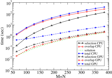
Figure 4: (Color online) The dependence of the computing time on CPU (solid lines) and GPU (dashed lines) (for the full solution and separate steps) on dimension of the basis $M=N$ for the $nd$ scattering problem with $S$-wave $NN$ interaction.

Fig. 4 shows the dependence of the CPU- and GPU-computing times for the above steps 2, 3, 5 and the complete solution for dimensions $M$ and $N$ of the WP bases chosen along both Jacobi variables. We take for simplicity $M=N$ in all of our tests so that, the total dimension of the matrix kernel is equal to $M^{2}$.

It is clear from Fig. 4 that the complete solution of $nd$ scattering problem in our approach for a basis of the large dimension $M=400$ takes only ca. 7 sec on a serial PC using GPU! This ultra-fast solution handles a huge matrix $160000\times 160000$ including the calculation of the ca. $M^{4}/100=256$ millions nonzero elements of matrix ${\mathbb{P}}^{0}$ where each matrix element is reduced to a integral of a rather complicated algebraic function. The integrals are calculated numerically with a 48-grid-point Gaussian quadrature.

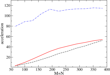
Figure 5: (Color online) The dependence of the GPU-acceleration ratio $\eta$ on the dimension of the basis $M=N$ in the calculation of the $nd$ scattering problem with a $S$-wave $NN$ interaction: dashed line shows the acceleration for the step 2 (selection), dot-dashed line — for the step 3 (calculation of ${\mathbb{P}}^{0}$), solid line — acceleration for the complete solution.

From Fig. 4 it is seen that all of these 256 million integrals can be computed on GPU in just 2.3 seconds compared to 255 seconds on the CPU. This demonstrates the real very high speed of GPU computations for the case discussed here.

In Fig. 5 we present the dependence of the GPU acceleration ratio $\eta=t(CPU)/t(GPU)$ on the dimension of the basis $M=N$ for the solution of the $S$-wave Faddeev problem. The total acceleration for the complete solution varies from 10 to 50 times depending on the basis dimension, while the time for calculating the nonzero elements of the matrix ${\mathbb{P}}^{0}$ (the step 3) which takes the main part of the CPU-computing time is reduced by a factor of more than 100.

We now turn to the case of the realistic $nd$ scattering problem with the Nijmegen $NN$ potential. Taking into account higher partial waves leads to the system of coupled two-dimensional integral Faddeev equations. Now the calculation of each matrix element of ${\mathbb{P}}^{0}$ for partial waves with nonzero angular momenta includes several tens of double numerical integrals with some trigonometric functions and uses a large set of algebraic coefficients $g^{l_{1}l^{\prime}_{1}k}_{\gamma\gamma^{\prime}}$ (49). The proper parallelization for this calculation with pre-selection of the nonzero matrix elements leads again to rather fast algorithm realized on GPU. Fig. 6 demonstrates the GPU acceleration ratio $\eta=t(CPU)/t(GPU)$ for the complete solution (solid line) and for the steps 2 (dashed line) and 3 (dot-dashed) as a function of the basis dimension $M=N$ for the solution of the 18-channel Faddeev equations for the $J=\frac{1}{2}^{+}$ partial $nd$ elastic amplitude.

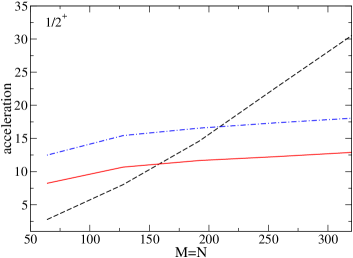
Figure 6: (Color online) The dependence of the GPU acceleration ratio $\eta$ on the dimension of the basis $M=N$ for the realistic $nd$ scattering problem for $J=\frac{1}{2}^{+}$: dashed line shows the acceleration for the step 2 (selection), dot-dashed line — for the step 3 (calculation of ${\mathbb{P}}^{0}$), solid line – the acceleration for the complete solution.

It is evident from the results presented that the passing from CPU- to GPU-realization on the same PC allows one to obtain a significant acceleration of whole three-body calculation by an order of magnitude or higher. It is clear also that the use of a more powerful specialized graphics processor, like the Tesla K40, would lead even to a considerably higher acceleration of calculations. However, it should be emphasized that the total acceleration which can be achieved by using GPU depends crucially on the method used, the numerical scheme and parallelization implementation.

VI Conclusion

In conclusion, let’s summarize the most important points of the proposed new general approach for the solution of few-body scattering problems.

1. First, we rewrite the initial Faddeev equations, which include an off-shell $t$-matrix, in a fully equivalent form which incorporates the product of the channel resolvent and the interaction operator. This allows us to simplify the required two-body input and also to fix all of the energy singularities in the channel resolvent operator. We note here that the four- and more particle integral Faddeev-Yakubovsky equations have, in principle, some similar structure as compared to three-body Faddeev equations (surely being more complicated and having a higher dimension). Therefore the discrete WP technique outlined in this paper can be employed for solving these general equations as well.

2. After that, we project out the transition and interaction operators onto a discrete wave-packet basis and employ a specific analytical form for one- and multi-channel resolvent operators. This discrete form is extremely convenient for few-body calculations because we get a fixed matrix form (with fully regular matrix elements) for the scattering equations (of Lippmann–Schwinger, Faddeev or Faddeev-Yakubovsky types). The most important improvement in such a WP projection is the fact that we can replace the permutation operators by fixed matrices, thus completely avoiding the numerous and time consuming interpolations at every iteration step. Moreover, this matrix is energy- and interaction-independent and, being calculated once, can be used to solve various scattering problems with different potentials and at many energies.

These two steps lead to a rather effective numerical scheme which is realized on a standard PC for realistic $3N$ scattering calculations.

3. At last, we perform a proper parallelization of the solution and eventually we employ the ultra-fast GPU technique to make very effective parallel calculations on a serial PC. This GPU realization for realistic scattering problems reduces the computational time by at least one order of magnitude (while for separate parts of the numerical scheme the total acceleration could reach two orders).

All of the above points open a new way for doing extensive many-body scattering calculations via continuum discretization e.g. in quantum chemistry, nuclear reaction theory, solid state theory etc..

There is little doubt that a similar (but surely more tedious) approach can also be applied to other scattering problems, e.g. to solve the relativistic Faddeev equations, Bethe–Salpeter equations etc.

Acknowledgments The authors thank Dr. A.V. Boreskov for discussions of problems associated with a use of the GPU. The authors are also deeply grateful to Prof. W. Polyzou for careful reading of the manuscript and valuable comments. This work has been supported partially by the Russian Foundation for Basic Research, grants Nos. 12-02-00908 and 13-02-00399.

Appendix A Calculation of permutation matrix elements.

The kernel of the permutation operator in momentum space has the form gloeckle

$$\langle pq\gamma|P|p^{\prime}q^{\prime}\gamma^{\prime}\rangle=\int_{-1}^{1}dx\frac{\delta(p^{\prime}-\pi_{1})\delta(p-\pi_{2})}{(p^{\prime})^{l^{\prime}+2}p^{l+2}}G_{\gamma\gamma^{\prime}}(q,q^{\prime},x),$$ (27)

where the multi-indices $\gamma$ and $\gamma^{\prime}$ include all possible spin-angular quantum numbers for the three-body states (as they are detailed in the Sec.IV , i.e. $\gamma=l,s,j,\lambda,I,J,\pi,t,T$) and the following notations

$$\pi_{1}=\sqrt{q^{2}+{\frac{1}{4}}(q^{\prime})^{2}+qq^{\prime}x},\ \pi_{2}=\sqrt{{\frac{1}{4}}q^{2}+(q^{\prime})^{2}+qq^{\prime}x},$$ (28)

are used. The spin-angular coefficients $G$ can be found from the formula

$$G_{\gamma\gamma^{\prime}}(q,q^{\prime},x)=\sum_{l_{1},l^{\prime}_{1},k}q^{l_{2}+l^{\prime}_{2}}(q^{\prime})^{l_{1}+l^{\prime}_{1}}P_{k}(x)g^{l_{1}l^{\prime}_{1}k}_{\gamma\gamma^{\prime}},\ \begin{array}[]{c}l_{1}+l_{2}=l,\\ l^{\prime}_{1}+l^{\prime}_{2}=l^{\prime},\\ \end{array}$$ (29)

where $l$ and $l^{\prime}$ are two-body subsystem orbital momenta and the indices $l_{1},l_{2},k,l^{\prime}_{1},l^{\prime}_{2}$ arise from intermediate triangle sums. The sum in (29) runs according to the triangle rules in partial coefficient $g^{l_{1}l^{\prime}_{1}k}_{\gamma\gamma^{\prime}}$ which have the following explicit form gloeckle :

$$g_{\gamma\gamma^{\prime}}^{l_{1}l^{\prime}_{1}k}=-\sqrt{\hat{l}\hat{s}\hat{j}\hat{t}\hat{\lambda}\hat{I}\hat{l^{\prime}}\hat{s^{\prime}}\hat{j^{\prime}}\hat{t^{\prime}}\hat{\lambda^{\prime}}\hat{I^{\prime}}}\left\{\begin{array}[]{ccc}\frac{1}{2}&\frac{1}{2}&t^{\prime}\\ \frac{1}{2}&T&t\end{array}\right\}\sum_{LS}(\hat{L}\hat{S})\times$$ (32)

$$\left\{\begin{array}[]{ccc}\frac{1}{2}&\frac{1}{2}&s^{\prime}\\ \frac{1}{2}&S&s\end{array}\right\}\left\{\begin{array}[]{ccc}l&s&j\\ \lambda&\frac{1}{2}&I\\ L&S&J\end{array}\right\}\left\{\begin{array}[]{ccc}l^{\prime}&s^{\prime}&j^{\prime}\\ \lambda^{\prime}&\frac{1}{2}&I^{\prime}\\ L&S&J\end{array}\right\}\times$$ (41)

$$\hat{k}\left(\frac{1}{2}\right)^{l^{\prime}_{2}+l_{1}}\sqrt{\frac{(2l+1)!}{(2l_{1})!(2l_{2})!}}\sqrt{\frac{(2l^{\prime}+1)!}{(2l^{\prime}_{1})!(2l^{\prime}_{2})!}}\times$$

$$\sum_{ff^{\prime}}\left\{\begin{array}[]{ccc}l^{\prime}_{1}&l^{\prime}_{2}&l^{\prime}\\ \lambda^{\prime}&L&f^{\prime}\end{array}\right\}\left\{\begin{array}[]{ccc}l_{2}&l_{1}&l\\ \lambda&L&f\end{array}\right\}\langle l^{\prime}_{2}0\lambda^{\prime}0|f^{\prime}0\rangle\langle l_{1}0\lambda 0|f0\rangle\times$$ (46)

$$\left\{\begin{array}[]{ccc}f^{\prime}&l^{\prime}_{1}&L\\ f&l_{2}&k\end{array}\right\}\langle k0l^{\prime}_{1}0|f0\rangle\langle k0l_{2}0|f^{\prime}0\rangle,$$ (49)

where the summation is done over all allowed intermediate quantum numbers. Projection of free three-body wave-functions $|p,q\rangle$ (plane waves) onto the WP states can be found (for the case of unit weights $f(p)$ and $\bar{f}(q)$) from the formula nd2 :

$$\langle p,q|{\mathfrak{p}}_{i}{\mathfrak{q}}_{j}\rangle=\frac{1}{\sqrt{d_{i}\bar{d}_{j}}}\frac{\theta(p\in\mathfrak{D}_{i})\theta(q\in\bar{\mathfrak{D}}_{j})}{pq}.$$ (50)

Here $d_{i}$, $\bar{d}_{j}$ are the widths of momentum intervals and function $\theta$ is analog of the Heaviside step-function: $\theta(p\in\mathfrak{D}_{i})=1$ if $p$ belongs to the interval $\mathfrak{D}_{i}$ and $\theta(p\in\mathfrak{D}_{i})=0$ otherwise.

To obtain the permutation matrix elements in the lattice basis (11), one should integrate kernel (27) over the lattice cells $\mathfrak{D}_{ij}$ and $\mathfrak{D}_{i^{\prime}j^{\prime}}$. These matrix elements are defined by the following integrals:

$$[{\mathbb{P}}_{0}]_{ij,i^{\prime}j^{\prime}}^{\gamma\gamma^{\prime}}\equiv\langle X_{ij}^{\gamma}|P|X_{i^{\prime}j^{\prime}}^{\gamma^{\prime}}\rangle=\sum_{kl_{1}l^{\prime}_{1}}\frac{g_{\gamma\gamma^{\prime}}^{kl_{1}l^{\prime}_{1}}}{\sqrt{d_{i}\bar{d}_{j}d_{i^{\prime}}\bar{d}_{j^{\prime}}}}\times$$

$$\int_{\mathfrak{D}_{ij}}dpdq\int_{\mathfrak{D}_{i^{\prime}j^{\prime}}}dp^{\prime}dq^{\prime}\int_{-1}^{1}dx\frac{q^{l_{2}+l^{\prime}_{2}+1}(q^{\prime})^{l_{1}+l^{\prime}_{1}+1}}{(p^{\prime})^{l^{\prime}+1}p^{l+1}}\times$$

$$\delta(p^{\prime}-\pi_{1})\delta(p-\pi_{2})P_{k}(x).\qquad$$ (51)

Using the Dirac delta-functions, the integrals over $p$ and $p^{\prime}$ are evaluated analytically:

$$[{\mathbb{P}}_{0}]_{ij,i^{\prime}j^{\prime}}^{\gamma\gamma^{\prime}}=\sum_{kl_{1}l^{\prime}_{1}}\frac{g_{\gamma\gamma^{\prime}}}{\sqrt{d_{i}\bar{d}_{j}d_{i^{\prime}}\bar{d}_{j^{\prime}}}}\int_{\bar{\mathfrak{D}}_{j}}dq\int_{\bar{\mathfrak{D}}_{j^{\prime}}}dq^{\prime}\int_{-1}^{1}dx\times$$

$$\frac{q^{l_{2}+l^{\prime}_{2}+1}(q^{\prime})^{l_{1}+l^{\prime}_{1}+1}}{(\pi_{1})^{l^{\prime}+1}(\pi_{2})^{l+1}}P_{k}(x)\theta(\pi_{1}\in\mathfrak{D}_{i^{\prime}})\theta(\pi_{2}\in\mathfrak{D}_{i}).\qquad$$ (52)

Further, the residual integrals can be evaluated in polar coordinates:

$$q=Q\cos\phi,\quad q^{\prime}=Q\sin\phi.$$ (53)

Then the matrix element takes the form:

$$[{\mathbb{P}}_{0}]_{ij,i^{\prime}j^{\prime}}^{\gamma\gamma^{\prime}}=\sum_{kl_{1}l^{\prime}_{1}}\frac{g_{\gamma\gamma^{\prime}}}{\sqrt{d_{i}\bar{d}_{j}d_{i^{\prime}}\bar{d}_{j^{\prime}}}}I,$$ (54)

where

$$I=\int_{-1}^{1}dxP_{k}(x)\int_{\phi_{1}}^{\phi_{2}}d\phi\frac{(\cos\phi)^{l_{2}+l^{\prime}_{2}+1}(\sin\phi)^{l_{1}+l^{\prime}_{1}+1}}{(\zeta_{1})^{l^{\prime}+1}(\zeta_{2})^{l+1}}\times$$

$$\int_{Q_{1}(\phi)}^{Q_{2}(\phi)}QdQ\ \theta\left(Q\in\frac{\mathfrak{D}_{i^{\prime}}}{\zeta_{1}}\right)\theta\left(Q\in\frac{\mathfrak{D}_{i}}{\zeta_{2}}\right),\qquad$$ (55)

and the following notations are employed:

$$\zeta_{1}=\sqrt{\cos^{2}\phi+{\frac{1}{4}}\sin^{2}\phi+x\cos\phi\sin\phi},$$

$$\zeta_{2}=\sqrt{{\frac{1}{4}}\cos^{2}\phi+\sin^{2}\phi+x\cos\phi\sin\phi}.$$ (56)

The boundaries of the integral area in $(Q,\phi)$-plane are defined by transformation of the rectangle in the $(q,q^{\prime})$-plane, so that:

$$\begin{array}[]{ll}\phi_{1}=\arctan\left(\frac{q^{\prime}_{j^{\prime}-1}}{q_{j}}\right),&Q_{1}(\phi)=\max\left(\frac{q_{j-1}}{\cos\phi},\frac{q^{\prime}_{j^{\prime}-1}}{\sin\phi}\right),\\ \phi_{2}=\arctan\left(\frac{q^{\prime}_{j^{\prime}}}{q_{j-1}}\right),&Q_{2}(\phi)=\min\left(\frac{q_{j}}{\cos\phi},\frac{q^{\prime}_{j^{\prime}}}{\sin\phi}\right).\\ \end{array}$$ (57)

Evaluating the $Q$-integral analytically, one gets the expression for the integral $I$:

$$I=\int_{-1}^{1}dxP_{k}(x)\int_{\phi_{1}}^{\phi_{2}}d\phi F_{ij,i^{\prime}j^{\prime}}(\phi,x)\times$$

$$\frac{(\cos\phi)^{l_{2}+l^{\prime}_{2}+1}(\sin\phi)^{l_{1}+l^{\prime}_{1}+1}}{(\zeta_{1})^{l^{\prime}+1}(\zeta_{2})^{l+1}},$$ (58)

where the following function is introduced:

$$F_{ij,i^{\prime}j^{\prime}}(\phi,x)={\frac{1}{2}}\left[\min\left(\frac{q_{j}}{\cos\phi},\frac{q^{\prime}_{j^{\prime}}}{\sin\phi},\frac{p^{\prime}_{i^{\prime}}}{\zeta_{1}},\frac{p_{i}}{\zeta_{2}}\right)\right]^{2}-$$

$${\frac{1}{2}}\left[\max\left(\frac{q_{j-1}}{\cos\phi},\frac{q^{\prime}_{j^{\prime}-1}}{\sin\phi},\frac{p^{\prime}_{i^{\prime}-1}}{\zeta_{1}},\frac{p_{i-1}}{\zeta_{2}}\right)\right]^{2}.\qquad\qquad$$ (59)

Finally, one gets the eventual formula for the permutation matrix

$$[{\mathbb{P}}_{0}]_{ij,i^{\prime}j^{\prime}}^{\gamma\gamma^{\prime}}=\sum_{kl_{1}l^{\prime}_{1}}\frac{g_{\gamma\gamma^{\prime}}^{kl_{1}l^{\prime}_{1}}}{\sqrt{d_{i}\bar{d}_{j}d_{i^{\prime}}\bar{d}_{j^{\prime}}}}\int_{-1}^{1}dxP_{k}(x)\times$$

$$\int_{\phi_{1}}^{\phi_{2}}d\phi F_{ij,i^{\prime}j^{\prime}}(\phi,x)\frac{(\cos\phi)^{l_{2}+l^{\prime}_{2}+1}(\sin\phi)^{l_{1}+l^{\prime}_{1}+1}}{(\zeta_{1})^{l^{\prime}+1}(\zeta_{2})^{l+1}}.$$ (60)

In practical treatments these integrals are evaluated numerically.

References

- (1) J. Carbonell, A. Deltuva, A.C. Fonseca, R. Lazauskas, Progr. Part. Nucl. Phys. 74, 55 (2014).
- (2) L.D. Faddeev, Sov. Phys.- JETP 12, 1014 (1961); O.A. Yakubovsky, Sov. J. Nuclear. Phys. 5, 937 (1967).
- (3) H. Witała, W.Glöckle, Phys. Rev. C 85, 064003 (2012).
- (4) https://developer.nvidia.com/cuda-zone
- (5) K.A. Wilkinson, P. Sherwood, M.F. Guest, K.J. Naidoo, J. Comp. Chem. 32, 2313 (2011).
- (6) M.A. Clark, R. Babich, K. Barrose, R.C. Brower, C. Rebbi, Comp. Phys. Com. 181, 1517 (2010).
- (7) H. Potter et al., Proceedings of NTSE-2013 (Ames, IA, USA, May 13-17 2013), Eds. A.M. Shirokov and A.I. Mazur, Khabarovsk, Russia, p. 263 (2014); http://www.ntse-2013.khb.ru/Proc/Sosonkina.pdf.
- (8) E. Yarevsky, LNCS 7125, Mathematical Modeling and Computational Science, Eds. A. Gheorghe, J. Buša and M. Hnatic, p. 290 (2012).
- (9) V.N. Pomerantsev, V.I. Kukulin, O.A. Rubtsova, Phys. Rev. C 79, 064602 (2009); ibid. 79, 034001 (2009).
- (10) O.A. Rubtsova, V.N. Pomerantsev, V.I. Kukulin, A. Faessler, Phys. Rev. C 86, 034004 (2012).
- (11) W. Glöckle, H. Witała, D.Hüber, H. Kamada, J. Golack, Phys. Rep. 274, 107 (1996).
- (12) V.G.J. Stoks, R.A.M. Klomp, C.P.F. Terheggen, J.J de Swart, Phys. Rev. C 49, 2950 (1994).
- (13) O.A. Rubtsova, V.I. Kukulin, V.N. Pomerantsev, A. Faessler, Phys. Rev. C 81, 064003 (2010).
- (14) M. Danos, W. Greiner, Phys. Rev. 146, 708 (1966).
- (15) O.A. Rubtsova, V.I. Kukulin, V.N. Pomerantsev, Physics of Atomic Nuclei 77, 486 (2014).
- (16) V.I. Kukulin, V.N. Pomerantsev, O.A. Rubtsova, Theor. Math. Phys. 150, 403 (2007).
- (17) S.N. Bunker et al., Nucl. Phys. A 113, 461 (1968).