The relation between gas density and velocity power spectra in galaxy clusters: qualitative treatment and cosmological simulations

Abstract

We address the problem of evaluating the power spectrum of the velocity field of the ICM using only information on the plasma density fluctuations, which can be measured today by Chandra and XMM-Newton observatories. We argue that for relaxed clusters there is a linear relation between the rms density and velocity fluctuations across a range of scales, from the largest ones, where motions are dominated by buoyancy, down to small, turbulent scales: $(\delta\rho_{k}/\rho)^{2}=\eta_{1}^{2}(V_{1,k}/c_{s})^{2}$, where $\delta\rho_{k}/\rho$ is the spectral amplitude of the density perturbations at wave number $k$, $V_{1,k}^{2}=V_{k}^{2}/3$ is the mean square component of the velocity field, $c_{s}$ is the sound speed, and $\eta_{1}$ is a dimensionless constant of order unity. Using cosmological simulations of relaxed galaxy clusters, we calibrate this relation and find $\eta_{1}\approx 1\pm 0.3$. We argue that this value is set at large scales by buoyancy physics, while at small scales the density and velocity power spectra are proportional because the former are a passive scalar advected by the latter. This opens an interesting possibility to use gas density power spectra as a proxy for the velocity power spectra in relaxed clusters, across a wide range of scales.

1. Introduction

Spectacular data accumulated by X-ray observatories on the nearest X-ray brightest clusters of galaxies allow us to probe inhomogeneities in the intracluster medium (ICM) over a broad range of spatial scales. These clusters typically show $\sim 5-10$% density fluctuations on scales from a few tens to a few hundred kpc (Churazov et al., 2012; Sanders & Fabian, 2012, see also Schuecker et al. 2004 for earlier work). At the same time, the dynamics of the ICM remain largely unknown. For relaxed clusters, numerical simulations predict predominantly subsonic motions of the ICM on scales from $\sim$Mpc down to a few tens of kpc with approximately Kolmogorov power spectra (PS) of the velocity field (see, e.g., Norman & Bryan, 1999; Dolag et al., 2005; Nagai et al., 2007b; Iapichino et al., 2011; Vazza et al., 2011).

The relatively low energy resolution ($\sim 130-150$ eV) of current X-ray CCD-type detectors precludes accurate measurements of gas velocities (see, e.g., Zhuravleva et al., 2013b; Tamura et al., 2014). The gain in resolution can be achieved in cool cores of clusters by using grating spectrometers. Such observations provide mostly upper limits on the gas velocities $\sim$ a few hundred km/s (e.g., Werner et al., 2009; Sanders & Fabian, 2013; Churazov et al., 2004). One can also use Faraday Rotation measurements to probe the ICM turbulence indirectly (e.g., Vogt & Enßlin, 2003).

The future Japanese-US X-ray observatory Astro-H (see Takahashi et al., 2010, launch in 2015) should provide high-resolution ($\sim 4-7$ eV) X-ray spectra, allowing one for the first time to measure gas velocities directly. However, it will not be trivial to extract the PS of the velocity field (see methods developed in Zhuravleva et al., 2012). The full power of the methods can only be used once the next generation of X-ray observatories, such as SMART-X and Athena+, are operating.

In the meantime, are there ways to probe the velocity PS with existing and near-term data? In this Letter, we argue that, for subsonic motions in relaxed clusters, there is a linear relation between the PS of density fluctuations derived from X-ray images, and the velocity PS. Using analytical description of a passive scalar advected by fluid motions in stratified medium, we show that the linearity holds from large scales, where motions are dominated by buoyancy, down to small, turbulent scales, with the same coefficient of proportionality. In turbulent regime linear dependence was found in simulations of massive cluster with solenoidal forcing in Gaspari & Churazov (2013). It is interesting that similar situations arise in the context of solar wind, Earth atmosphere, and the ISM (see, e.g. Armstrong et al., 1995).

Churazov et al. (2012) list the following contributions to measured density variations in clusters: (1) perturbations of the gravitational potential; (2) deviations from the oversimplified model profiles; (3) entropy fluctuations caused by infalling low-entropy gas or by gas advection; (4) pressure variations associated with gas motions and sound waves; (5) metallicity variations; (6) the presence of non-thermal and spatially variable components. Cosmological simulations of relaxed clusters (Section 3), which include effects (1)–(4), illustrate that predicted linearity holds approximately in the case of “natural” cosmological driving. In the companion paper (Gaspari et al., 2014, hereafter G14), high-resolution simulations in a static gravitational potential with solenoidal forcing of turbulence are used to investigate items (3) and (4) and the role of isotropic thermal conduction.

2. Velocity field and density fluctuations

Let us consider slow, subsonic gas motions in a cluster potential. Two different regimes can be distinguished: (i) a large-scale limit, where the dynamics are governed by buoyancy and (ii) a turbulent regime at small scales, where the eddy turnover time is shorter than the characteristic buoyancy time scale. Below, we argue that there is a linear relation with the same constant of proportionality between the amplitudes of the gas density and velocity fluctuations in both regimes.

2.1. Buoyancy-dominated regime (large scales)

Assuming that the ICM can be described by standard hydrodynamics (or magnetohydrodynamics), the entropy $s=P/\rho^{\gamma}$ (where $P$ is pressure, $\rho$ density and $\gamma=5/3$ the adiabatic index) satisfies

$$\frac{\partial s}{\partial t}+{\bf V}\cdot\nabla s=0,$$ (1)

where ${\bf V}$ is the flow velocity and we have neglected any heat fluxes, heating or cooling of the ICM. In a static equilibrium, the entropy has a radial profile $s_{0}(r)$ (a stratified atmosphere in a gravitational well). As the ICM is turbulent, this profile will be perturbed on scales that are smaller than the scale height $H_{s}=(d\ln s_{0}/dr)^{-1}$ — and if we assume that the ICM motions are subsonic, $V\ll c_{s}=\sqrt{\gamma P_{0}/\rho_{0}}$, these perturbations will be small: $s=s_{0}+\delta s$, $\delta s/s_{0}\ll 1$. They satisfy

$$\left(\frac{\partial}{\partial t}+{\bf V}\cdot\nabla\right)\frac{\delta s}{s_{0}}=-\frac{V_{r}}{H_{s}},$$ (2)

where $V_{r}$ is the radial velocity perturbation.

If all perturbations, including $V/c_{s}$, were infinitesimal, the restoring buoyancy force on a gas element displaced in the radial direction would result in oscillatory motions — gravity waves, or g-modes. Their frequency is

$$\omega=\frac{k_{\perp}}{k}\,N,\quad N=\sqrt{\frac{g}{\gamma H_{s}}}=\frac{c_{s}}{\gamma\sqrt{H_{s}H_{p}}},$$ (3)

where $k$ is the wave number of the oscillations, $k_{\perp}$ its projection perpendicular to the radial direction, $N$ is the Brunt-V$\ddot{\rm a}$is$\ddot{\rm a}$l$\ddot{\rm a}$ frequency, $g$ is the acceleration of gravity, $H_{p}=(d\ln P_{0}/dr)^{-1}$ is the pressure scale height, and the last equality follows from the hydrostatic force balance, $dP_{0}/dr=\rho_{0}g$. The density perturbations associated with these motions are

$$\left(\frac{\delta\rho}{\rho}\right)^{2}=\left(\frac{1}{\gamma}\frac{\delta s}{s}\right)^{2}=\left(\frac{V_{r}}{\gamma\omega H_{s}}\right)^{2}=\frac{H_{p}}{H_{s}}\frac{k^{2}}{k_{\perp}^{2}}\left(\frac{V_{r}}{c_{s}}\right)^{2},$$ (4)

which follows from equation (2) if the advection term is neglected; we have suppressed $0$’s in the subscripts of equilibrium quantities. The relationship between $\delta\rho/\rho$ and $\delta s/s$ is a consequence of local pressure balance ($\delta P/P\ll\delta\rho/\rho$), which holds for subsonic motions.

In reality, perturbations are not infinitesimal and the question is to what extent the linear relationship between density and velocity survives in the strongly nonlinear regime, when the advection term in equation (2) is not negligible. The argument that this relationship does survive depends somewhat nontrivially on the strength of the ICM turbulence at the outer (energy-injection) scale. The key parameter is the Froude number,

$${\rm Fr}=\frac{V_{\rm rms}}{L_{\perp}N}={\rm Ma}\,\frac{\gamma\sqrt{H_{s}H_{p}}}{L_{\perp}},$$ (5)

the ratio of the nonlinear decorrelation and linear Brunt-V$\ddot{\rm a}$is$\ddot{\rm a}$l$\ddot{\rm a}$ frequencies at the outer scale ($V_{\rm rms}$ is the rms velocity of the turbulent motions, ${\rm Ma}=V_{\rm rms}/c_{s}$ is the Mach number and $L_{\perp}$ is the outer scale perpendicular to the radial direction).

If ${\rm Fr}\ll 1$, the turbulence will tend to a stratified, anisotropic regime, in which $k_{\perp}\ll k\approx k_{r}$ and the gravity-wave frequency $\omega=Nk_{\perp}/k\ll N$ stays comparable to the nonlinear decorrelation rate $k_{\perp}V_{\perp}$ (a type of “critically balanced” state; see Lindborg, 2006; Nazarenko & Schekochihin, 2011). In this regime, buoyancy remains important scale by scale ($k$ by $k$) as the energy cascades to smaller scales (larger $k$), the relationship (4) is approximately satisfied, and the typical velocity of the motions is dominated by the perpendicular velocity: $V\sim V_{\perp}\sim(k_{r}/k_{\perp})V_{r}\gg V_{r}$ (by incompressibility). Therefore, we deduce, at each $k$,

$$\left(\frac{\delta\rho_{k}}{\rho}\right)^{2}=\eta^{2}\left(\frac{V_{k}}{c_{s}}\right)^{2},$$ (6)

where $\eta$ is a scale-independent dimensional constant of order unity. Here $\delta\rho_{k}$ and $V_{k}$ are some suitably defined fluctuation amplitudes at scale $k^{-1}$ (see Section 3.2), rather than Fourier components, they are related to the 3D spectrum $E_{k}$ by $|V_{k}|^{2}\sim kE_{k}$.

For this kind of turbulence, it is possible to show (see Lindborg, 2006; Nazarenko & Schekochihin, 2011, and references therein) that the energy spectrum of the perpendicular motions (and, therefore, of the density perturbations) is Kolmogorov in the perpendicular direction, $E_{k}\sim\varepsilon^{2/3}k_{\perp}^{-5/3}$, where $\varepsilon$ is the energy flux, and much steeper in the radial direction, $E_{k}\sim N^{2}k_{r}^{-3}$ (Dewan, 1997; Billant & Chomaz, 2001), but that as the turbulent cascade proceeds to smaller scales, turbulence becomes less anisotropic, eventually reaching isotropy ($k_{\perp}\sim k_{r}$, $V_{\perp}\sim V_{r}$) at the so-called Ozmidov scale, $k\sim k_{\rm O}=N^{3/2}\varepsilon^{-1/2}$, where the perpendicular and radial spectra meet and the “local” Froude number is $V_{k_{\rm O}}k_{\rm O}/N\sim 1$ (Ozmidov 1992; for the latest numerical results, see Augier et al. 2012). Beyond this scale ($k>k_{\rm O}$), the stratified cascade turns into the usual isotropic Kolmogorov cascade, in which $k_{\perp}\sim k_{r}$, $V_{r}\sim V_{\perp}$, $E_{k}\sim\varepsilon^{2/3}k^{-5/3}$, the nonlinear decorrelation rate becomes dominant compared to the linear gravity-wave frequency $\omega\sim N$ — and the relation (6) continues to be satisfied, but for reasons unrelated to the buoyancy physics and considered in Section 2.2.

If ${\rm Fr}\sim 1$ at the outer scale, the turbulence can be assumed isotropic, with $k_{\perp}\sim k_{r}\sim k$ and $V_{r}\sim V_{\perp}\sim V_{\rm rms}$ already at $kL_{\perp}\sim 1$, and so the relation (6) is satisfied at the outer scale. Again, it will continue to be satisfied at $kL>1$, as we are about to explain. This is probably the more common situation: in relaxed clusters (see Table 1), ${\rm Fr}\sim 0.3\left(L_{\perp}/300~{}{\rm kpc}\right)^{-1}\sim 0.3-1$.

Thus, in the entire interval of scales where buoyancy matters (which may or may not extend beyond the outer scale, depending on the value of ${\rm Fr}$), one can expect a linear relation between the velocity and the density perturbation with a coefficient of order unity, equation (6).

2.2. Turbulent regime (small scales)

Consider now the limit of small scales, $k>k_{\rm O}$. At these scales (the “inertial range”), the nonlinear decorrelation (eddy turnover) rate becomes increasingly (with $k$) greater than the Brunt-V$\ddot{\rm a}$is$\ddot{\rm a}$l$\ddot{\rm a}$ frequency. This means that the right-hand side of equation (2) can be neglected and so the entropy fluctuations are a passive scalar field. Since $\delta\rho/\rho=-(1/\gamma)\delta s/s$, so are the density fluctuations.

A scaling theory for such passive fluctuations in the inertial range can be constructed along the lines of the Obukhov–Corrsin theory (Obukhov, 1949; Corrsin, 1951). The total variance of $\delta\rho/\rho$ is conserved, and so there should be a constant flux $\varepsilon_{\rho}$ of it towards smaller scales:

$$\left(\frac{\delta\rho_{k}}{\rho}\right)^{2}\sim\frac{\varepsilon_{\rho}\tau_{k}}{c_{s}^{2}},$$ (7)

where $\varepsilon_{\rho}$ is the scalar dissipation rate, $\tau_{k}$ is the typical “cascade time” and $c_{s}^{2}$ appears in the right-hand side simply to ensure convenient normalization of the flux $\varepsilon_{\rho}$ to energy units. Similarly, for the turbulent motions themselves,

$$V_{k}^{2}\sim\varepsilon_{V}\tau_{k},$$ (8)

where $\varepsilon_{V}$ is the flux of the kinetic energy and $\tau_{k}$ is the same cascade time as in equation (7) because both $\delta\rho/\rho$ and ${\bf V}$ are mixed by the same velocity field. From equation (8), $\tau_{k}\sim V_{k}^{2}/\varepsilon$ and, therefore, from equation (7),

$$\left(\frac{\delta\rho_{k}}{\rho}\right)^{2}\sim\frac{\varepsilon_{\rho}}{\varepsilon_{V}}\left(\frac{V_{k}}{c_{s}}\right)^{2}.$$ (9)

Thus, the spectrum of the passive scalar follows the spectrum of the velocity field in the inertial range. The constant of proportionality in equation (9), $\varepsilon_{\rho}/\varepsilon_{V}$, depends on how much scalar variance, compared to kinetic energy, arrives into the inertial range from the larger, buoyancy-dominated scales. Therefore, the relationship (9) should be matched with (6): $\varepsilon_{\rho}/\varepsilon_{V}\sim\eta^{2}$.

Note that these conclusions are independent of what precisely the spectrum of the turbulence is because the argument above was based only on the assumption that the cascade times are the same for the passive scalar and for the turbulence that advects it. This is reassuring because ICM turbulence is certainly not a simple hydrodynamic Kolmogorov turbulence of an inertial fluid. At the very least, it is magnetohydrodynamic, as clusters are known to host dynamically significant magnetic fields (see e.g., Schekochihin & Cowley, 2006; Enßlin & Vogt, 2006, and references therein). Since $\beta=8\pi P/B^{2}\sim 10^{2}\gg 1$, these fields do not significantly modify buoyancy physics at large scales. In the inertial range, the turbulence may be MHD rather than hydrodynamic, but density fluctuations continue to behave as a passive scalar in Alfvénic MHD and even kinetic turbulence (Schekochihin & Cowley, 2007; Schekochihin et al., 2009) and so the above argument continues to hold.

Thus, the conclusion from this section is that the relation (6) holds with the same proportionality constant both at scales where buoyancy physics matters and at those where it does not and independently of whether ${\rm Fr}$ is small or order unity (i.e., independently of how vigorous the turbulence is and of whether it is isotropic Kolmogorov turbulence or anisotropic stratified one). Below, we verify these arguments using a sample of cosmological hydrodynamic simulations of galaxy clusters.

Table 1Sample of simulated galaxy clusters

ClusterID	r500c, kpc	M500c, 1014$\cdot$M⊙	Ma
CL149	814.4	1.83	0.48
CL21	1215.2	6.08	0.21
CL223	824	1.9	0.29
CL25	1095.8	4.46	0.32
CL27	1154.5	5.21	0.23
CL42	1297.7	7.4	0.27

Note. — Mach number ${\rm Ma}=V_{\rm rms}/c_{s}$ is calculated as the RMS of the velocity in the central 500 kpc after subtracting the mean velocity in this region.

3. Calibration with cosmological simulations

3.1. Simulations and sample of galaxy clusters

We use high-resolution cosmological simulations of galaxy clusters in a flat $\Lambda$CDM model with WMAP five-year cosmological parameters: $\Omega_{m}=1-\Omega_{\Lambda}=0.27$, $\Omega_{b}=0.0469$, $h=0.7$ and $\sigma_{8}=0.82$. The simulations are performed using the Adaptive Refinement Tree (ART) $N$-body+gas-dynamics code (Kravtsov, 1999; Kravtsov et al., 2002; Rudd et al., 2008), which is an Eulerian code that uses adaptive refinement in space and time and non-adaptive refinement in mass (Klypin et al., 2001) to achieve the dynamic ranges necessary to resolve the cores of halos formed in self-consistent cosmological simulations. Details of the zoom-in simulations used here can be found in Nelson et al. (2014, Section 3.1).

Our sample includes 6 relaxed clusters at $z=0$. Their X-ray morphology exhibits spherical or elliptical symmetry with no filamentary or clumpy substructures within $r_{500c}$ (see Nagai et al., 2007a). We analyze non-radiative (NR) runs only, because these involve physical processes directly relevant to those discussed in Section 2.

We analyze fluctuations in the central $\sim 500$ kpc (radius) region. The gas motions are subsonic with ${\rm Ma}\sim 0.2-0.5$ (Table 1). X-ray images of the NR relaxed clusters do not show any prominent subhaloes or clumpy structures within $\sim 500$ kpc (Fig. 1, inset). Only cluster CL25 has a small subhalo, which we remove from the analysis. Subhaloes/clumps, which are present in 3D data and are not visible in projection, only slightly affect our results. E.g., for cluster CL149 the exclusion of clumps with $\delta\rho/\rho>1$ removes $\sim$1.8% of the volume and changes the total rms of $\delta\rho/\rho$ by $\sim$10%. The changes in ${\rm Ma}$ are less than 1%.

Figure 1.— X-ray surface brightness (2$\times$2 Mpc) of simulated cluster CL21 (inset), and its radial profile (main plot, red points). Black curve: best-fitting $\beta$ model. Vertical dash lines: the fitting interval.

3.2. Power spectra of density and velocity fluctuations

For each cluster in our sample, we calculated the 3D emissivity-weighted electron density as $\displaystyle n_{e,X}=n_{e}\sqrt{\Lambda(T)}$, where $\Lambda(T)$ is the gas emissivity (Sutherland & Dopita, 1993), and three components of the normalized velocity field, $V_{x,y,z}/c_{s}$. Projecting the squared density along one of the directions, the X-ray surface brightness (SB), $I_{X}(x,y)\propto\displaystyle\int n_{e,X}^{2}(x,y,z)dz$, is obtained. We calculate the spherically-symmetric radial profile of the SB, and approximate it with a $\beta$ model (Fig. 1). Dividing the density by the corresponding 3D $\beta$ model and subtracting unity, the 3D density fluctuations ${\delta\rho}/{\rho}$ are obtained. The center of each cluster is chosen as the peak of the gas density within the central $\sim 50$ kpc region and confirmed by the visual inspection.

We then use the modified $\Delta-$variance method (Arévalo et al., 2012) to calculate $P_{3D}(k)$, the PS of the 3D density fluctuations and velocity. These spectra are converted to fluctuations amplitudes $A_{k}=\sqrt{4\pi P_{3D}(k)k^{3}}$. Fig. 2 shows an example of such amplitudes of the density fluctuations $\delta\rho_{k}/\rho$ and of rms velocity component $V_{1,k}=\sqrt{(V_{x,k}^{2}+V_{y,k}^{2}+V_{z,k}^{2})/3}$ for cluster CL21. These amplitudes follow each other over a broad range of scales. Their ratio $\eta_{1}=({\delta\rho_{k}}/{\rho})/({V_{1,k}}/c_{s})$ is close to unity with $\sim 10$% deviations.

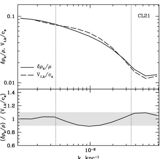
Figure 2.— Amplitudes of density and velocity fluctuations (top panel) and their ratio (bottom panel) for CL21 cluster. A convention $k=1/\lambda$ without a factor $2\pi$ is used throughout. The ratio is consistent with unity with a scatter $<$ 10% (gray shaded region) at scales $\sim 30-300$ kpc (vertical dotted lines), which are least affected by numerical artifacts (see Section 3.2).

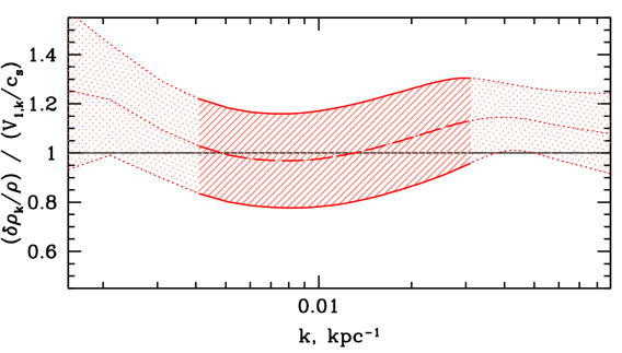
Figure 3.— Sample-averaged ratio of the amplitudes of density and velocity fluctuations. Shaded region: scatter over the sample. Solid curves and shadows: the range of scales least affected by numerical artifacts (see Section 3.2). The ratio is $\eta_{1}=1\pm 0.3$ at scales $\sim 30-300$ kpc^-1.

Even though the relationship (6) is found to hold over a broad range of scales, the amplitudes at the smallest and the largest scales are affected by several artifacts. At $k\gtrsim 4\cdot 10^{-2}$ kpc^-1, the limit of numerical resolution is reached. At the largest scales, the amplitude is (a) sensitive to the underlying model used to correct for the global structure of the cluster; (b) affected by uncertainties due to stochastic nature of perturbations. The sensitivity to (a) is estimated by experimenting with different underlying models (e.g., non-spherical $\beta$ models, averaged profiles). In order to evaluate the uncertainties (b), we experimented with multiple realizations of a Gaussian field that had a PS similar to that of density/velocity fluctuations in simulated clusters. As expected there are large variations at $k\sim 1/L$, where $L=1000$ kpc is the size of the box. At $k\geq 3/L\sim 3\cdot 10^{-3}~{}{\rm kpc}^{-1}$ the variations drop down to $\sim 5-10$%.

The ratio $\eta_{1}$ of the amplitudes of density and velocity fluctuations averaged over a sample of relaxed clusters is shown in Fig. 3. It is consistent with $\eta_{1}=1$ at scales $\sim 30-300$ kpc, with a relatively modest scatter $\lesssim$30%. There are many possible reasons for this scatter. In particular, the presence of individual subhaloes, the choice of the cluster center and the underlying model, effects of AMR resolution and of finite ${\rm Ma}$ (see G14) can all contribute to variations at this level.

In order to assess the effects of the AMR resolution on our results, we resimulated one cluster, varying the maximum refinement levels from 6 to 9 (the default one is 8). In the lowest-resolution runs, both density and velocity fluctuations are suppressed compared to the high-resolution runs at all scales, except for the largest $\sim 300$ kpc. The amplitudes of density fluctuations in simulations with the refinement levels 8 and 9 globally follow each other at scales $\sim$ 50-300 kpc. However, at some scales, deviations are up to a factor 1.3. The velocity amplitudes are the same at scales $\sim 300-100$ kpc and differ by a factor 1.5 at $\sim 50$ kpc. Despite individual PS varying with the AMR resolution, the ratio of density and velocity fluctuations in all runs is still close to unity, with the scatter up to 25% at scales $\sim 50-300$ kpc.

4. Conclusions

In this Letter, we have addressed the problem of constraining the gas velocity PS in relaxed galaxy clusters using the observed density fluctuations. We argue that

• the rms of density and velocity fluctuations are linearly related across a broad range of scales in both buoyancy-dominated and turbulent regimes;

• the constant of proportionality between them is set at large scales by gravity-wave physics and remains approximately the same in the non-linear turbulent regime;

• cosmological simulations of relaxed clusters give a proportionality coefficient $\eta_{1}\sim 1\pm 0.3$ between the amplitude of the density fluctuations and the rms component of the flow velocity;

It is an interesting conclusion that, if the energy-injection scales are large enough (e.g., $\sim 10^{2}$ kpc for merger-driven turbulence), stratification leads to anisotropy ($V_{\perp}\gg V_{r}$, $k_{\perp}\ll k_{r}$), whereas turbulence driven at small scales (e.g., $\sim 10$ kpc, as in the AGN-driven case) will be isotropic—these are the ${\rm Fr}\ll 1$ and ${\rm Fr}\sim 1$ cases discussed in Section 2.1. Indeed, in cosmological simulations, where turbulence is primarily driven by mergers, we see perpendicular velocities slightly larger than the radial ones in the central 500 kpc.

Admittedly, our simulations suffer from insufficient dynamic range and do not include all relevant physical processes. For instance, thermal conduction could erase some of the temperature/density fluctuations and break the relation (6). Some of these effects are considered in the companion paper (G14), where a series of high-resolution hydrodynamic simulations is carried out, with varying ${\rm Ma}$ and isotropic conductivity.

It should be possible to verify the relation (6) using future direct velocity measurements with Astro-H (combining with current observations). Strong deviations from $\eta\sim 1$ would suggest interesting microphysics or the dominance of other sources of density fluctuations.

In conclusion we have shown that the analysis of SB fluctuations in X-ray images offers a novel way to estimate the velocity PS in relaxed galaxy clusters. In general, proportionality between the density and velocity amplitudes for subsonic motions is probably a generic feature of small perturbations in stratified atmospheres.

References

- Arévalo et al. (2012) Arévalo, P., Churazov, E., Zhuravleva, I., Hernández-Monteagudo, C., & Revnivtsev, M. 2012, MNRAS, 426, 1793
- Armstrong et al. (1995) Armstrong, J. W., Rickett, B. J., & Spangler, S. R. 1995, ApJ, 443, 209
- Augier et al. (2012) Augier, P., Cmomaz, J.-M., & Billant, P. 2012, J. Fluid Mech., 713, 86
- Balbus (2000) Balbus, S. A. 2000, ApJ, 534, 420
- Billant & Chomaz (2001) Billant, P. & Cmomaz, J.-M., 2001, Phys. Fluids, 13, 1645
- Churazov et al. (2004) Churazov, E., Forman, W., Jones, C., Sunyaev, R., Böhringer, H. 2004, MNRAS, 347, 29
- Churazov et al. (2012) Churazov, E., Vikhlinin, A., Zhuravleva, I., et al. 2012, MNRAS, 421, 1123
- Corrsin (1951) Corrsin S. 1951, Journal of Applied Physics, 22, 469
- Dewan (1997) Dewan, E., 1997, J. Geophys. Res., 102, 29799
- Dolag et al. (2005) Dolag, K., Vazza, F., Brunetti, G., & Tormen, G. 2005, MNRAS, 364, 753
- Enßlin & Vogt (2006) Enßlin, T. A. & Vogt, C. 2006, A&A, 453, 447
- Gaspari & Churazov (2013) Gaspari, M., & Churazov, E. 2013, A&A, 559, A78
- Iapichino et al. (2011) Iapichino, L., Schmidt, W., Niemeyer, J. C., & Merklein, J. 2011, MNRAS, 414, 2297
- Klypin et al. (2001) Klypin, A., Kravtsov, A. V., Bullock, J. S., & Primack, J. R. 2001, ApJ, 554, 903
- Kravtsov (1999) Kravtsov, A. V. 1999, Ph.D. Thesis, New Mexico State Univ.
- Kravtsov et al. (2002) Kravtsov, A. V., Klypin, A., & Hoffman, Y. 2002, ApJ, 571, 563
- Kunz (2011) Kunz, M. W. 2011, MNRAS, 417, 602
- Lindborg (2006) Lindborg, E., 2006, J. Fluid Mech., 550, 207
- Nagai et al. (2007a) Nagai, D., Kravtsov, A. V., & Vikhlinin, A. 2007, ApJ, 668, 1
- Nagai et al. (2007b) Nagai, D., Vikhlinin, A., & Kravtsov, A. V. 2007, ApJ, 655, 98
- Nazarenko & Schekochihin (2011) Nazarenko, S. V., Schekochihin, A. A., 2011, J. Fluid Mech., 677, 134
- Nelson et al. (2014) Nelson, K., Lau, E. T., Nagai, D., Rudd, D. H., & Yu, L. 2014, ApJ, 782, 107
- Norman & Bryan (1999) Norman, M. L., & Bryan, G. L. 1999, The Radio Galaxy Messier 87, 530, 106
- Obukhov (1949) Obukhov, A. M. 1949, Izv. Akademii Nauk SSSR, Geogr. Geofiz., 13, 58
- Ozmidov (1992) Ozmidov, R. V., 1992, Oceanology, 32, 259
- Rudd et al. (2008) Rudd, D. H., Zentner, A. R., & Kravtsov, A. V. 2008, ApJ, 672, 19
- Quataert (2008) Quataert, E. 2008, ApJ, 673, 758
- Sanders & Fabian (2012) Sanders, J. S., & Fabian, A. C. 2012, MNRAS, 421, 726
- Sanders & Fabian (2013) Sanders, J. S., & Fabian, A. C. 2013, MNRAS, 429, 2727
- Schuecker et al. (2004) Schuecker, P., Finoguenov, A., Miniati, F., Böhringer, H., & Briel, U. G. 2004, A&A, 426, 387
- Schekochihin & Cowley (2006) Schekochihin, A. A. & Cowley, S. C. 2006, Phys. Plasmas, 13, 056501
- Schekochihin & Cowley (2007) Schekochihin, A. A. & Cowley, S. C. 2007, in Magnetohydrodynamics: Historical Evolution and Trends, ed. by S. Molokov, R. Moreau and H. K. Moffatt. (Dordrecht: Springer) p. 85
- Schekochihin et al. (2009) Schekochihin, A. A., Cowley, S. C., Dorland, W., Hammett, G. W., Howes, G. G., Quataert, E., & Tatsuno, T. 2009, ApJS, 182, 310
- Sutherland & Dopita (1993) Sutherland, R. S., & Dopita, M. A. 1993, ApJS, 88, 253
- Takahashi et al. (2010) Takahashi, T., Mitsuda, K., Kelley, R., et al. 2010, Proc. SPIE, 7732,
- Tamura et al. (2014) Tamura, T., Yamasaki, N. Y., Iizuka, R., et al. 2014, ApJ, 782, 38
- Vazza et al. (2011) Vazza, F., Brunetti, G., Gheller, C., Brunino, R., & Brüggen, M. 2011, A&A, 529, A17
- Vogt & Enßlin (2003) Vogt, C., & Enßlin, T. A. 2003, A&A, 412, 373
- Werner et al. (2009) Werner, N., Zhuravleva, I., Churazov, E., et al. 2009, MNRAS, 398, 23
- Zhuravleva et al. (2012) Zhuravleva, I., Churazov, E., Kravtsov, A., & Sunyaev, R. 2012, MNRAS, 422, 2712
- Zhuravleva et al. (2013b) Zhuravleva, I., Churazov, E., Sunyaev, R., et al. 2013, MNRAS, 435, 3111