Catastrophe versus instability for the eruption of a toroidal solar magnetic flux rope

Abstract

The onset of a solar eruption is formulated here as either a magnetic catastrophe or as an instability. Both start with the same equation of force balance governing the underlying equilibria. Using a toroidal flux rope in an external bipolar or quadrupolar field as a model for the current-carrying flux, we demonstrate the occurrence of a fold catastrophe by loss of equilibrium for several representative evolutionary sequences in the stable domain of parameter space. We verify that this catastrophe and the torus instability occur at the same point; they are thus equivalent descriptions for the onset condition of solar eruptions.

1. Introduction

The force-free equilibrium of a coronal magnetic flux rope that carries a net current requires the presence of an external poloidal field perpendicular to the current (Shafranov, 1966; van Tend & Kuperus, 1978). Magnetic flux associated with the current is squeezed between the current and the photospheric boundary. This can be described as an induced current in the boundary or, equivalently, as an oppositely directed image current, implying an upward Lorentz force on the coronal flux (Kuperus & Raadu, 1974). The force is balanced by a Lorentz force from the external poloidal field.

As the photospheric flux distribution and the corresponding external field gradually change, the configuration evolves quasi-statically along a sequence of stable equilibria for most of the time. However, it may encounter an end point of such a sequence, where continuing photospheric changes trigger a dynamic evolution. The transition of an equilibrium flux rope to a state of non-equilibrium has become a standard model for the onset of eruptive phenomena, including the eruption of prominences, coronal mass ejections, and flares. It has been formulated as a catastrophe or as an instability in the framework of ideal magnetohydrodynamics (MHD).

The formulation as catastrophe involves a sequence of equilibria, i.e., the equilibrium manifold in parameter space, and an “evolutionary scenario” for the motion of the system point on the manifold as a control parameter evolves continuously (representing gradual changes at the boundary). Thus, it includes a model for the pre-eruptive evolution. A catastrophe occurs if the system point encounters a critical point on the equilibrium manifold. Most relevant for solar eruptive phenomena is the case that the critical point is an end point, or nose point, of the equilibrium manifold in the direction of the changing parameter. The catastrophe then occurs by a loss of equilibrium, sometimes also referred to as “non-equilibrium”.

The formulation as instability considers the evolution of a small perturbation acting on an equilibrium at any point on the equilibrium manifold. A full description of instability includes the temporal evolution of the perturbation, but in order to find a criterion for onset of eruption, only the point(s) of marginal stability must be located in parameter space. As a parameter changes, the system point moves from the stable part of the equilibrium manifold across a point of marginal stability to the unstable part, i.e., in this formulation the equilibrium is not lost but turns to an unstable equilibrium. A model for the pre-eruptive evolution does not enter here; the points of marginal stability are independent of the pre-eruptive evolution.

The modeling of solar eruptions has so far mostly used either a catastrophe formulation or an instability formulation, although they are related to each other. An analysis of this relationship should be helpful for unifying some of the independent developments in the modeling, which we summarize next.

A model of eruption onset from the force-free equilibrium of a flux rope was established by van Tend & Kuperus (1978) who focused on instability, but also related the instability to the fact that the equilibrium may be lost (see also Molodenskii & Filippov, 1987). They considered a translationally invariant coronal current in the center of a magnetic flux rope above a plane photospheric surface. The current was approximated as a line current immersed in an external poloidal field $B_{\mathrm{e}}$, and only its external, large-scale equilibrium was analyzed. It was found that the height dependence $B_{\mathrm{e}}(h)$ determines whether the configuration is stable or unstable. The current is unstable to an upward displacement if $B_{\mathrm{e}}$ decreases sufficiently rapidly with height $h$ above the boundary surface. In the two-dimensional (2D) translationally invariant geometry, the “decay index” $n=-d\ln B_{\mathrm{e}}/d\ln h$ must exceed $n_{\mathrm{cr}}=1$ for instability. This critical value was derived under the assumption that any change of current produced by the perturbation can be neglected, which is consistent with conservation of magnetic flux between the current channel and the boundary surface in the limit of vanishing current channel radius $a$ (Forbes, 1990). A slightly higher value results if the constraint of flux conservation is imposed for $a>0$; then $n_{\mathrm{cr}}=1+1/(2c)$, where $c=\ln(2h/a)+1$ (Démoulin & Aulanier, 2010).

An MHD description of the configuration, including internal force-free equilibrium of the current channel, was developed by Priest & Forbes (1990) and Forbes & Isenberg (1991) and further elaborated in a series of papers by Isenberg et al. (1993), Forbes & Priest (1995), Lin & Forbes (2000), and Lin & van Ballegooijen (2002). All of these investigations described the onset of eruption as the occurrence of a catastrophe. The condition of flux conservation between the current channel and the photosphere was adopted in some cases, but other assumptions were considered as well, in order to model the changes in photospheric flux budget (flux cancellation or emergence) which are often observed in the pre-eruption phase (Martin et al., 1985; Feynman & Martin, 1995). Various evolutionary scenarios and external field models were analyzed. Accordingly, various locations of the critical point in parameter space were obtained.

More recently, Longcope & Forbes (2014) have found that a flux rope in quadrupolar external field can reach a catastrophe along various evolutionary paths, depending on the detailed form of the initial equilibrium. Some equilibria can be driven to a catastrophe and instability through reconnection at a lower, vertical current sheet, a process often referred to as “tether cutting” (Moore et al., 2001). While other equilibria can be driven to a catastrophe and instability through reconnection at an upper, horizontal current sheet, a process referred to as “breakout” (Antiochos et al., 1999). Some equilibria can be destabilized by both processes, but others only by one and not the other. Still other equilibria undergo no catastrophe and instability, but evolve at an increasingly rapid rate in response to slow steady driving.

The occurrence of a catastrophe has also been demonstrated for toroidal current channels. Lin et al. (1998) considered a toroidal flux rope encircling the Sun in the equatorial plane with an induced current in the solar surface, or equivalently, an image inside the Sun of the current channel. Lin et al. (2002) studied a toroidal current channel one half of which is submerged below the (plane) photosphere. In this geometry, the submerged half of the channel represents the image current, but the evolution of the channel’s major radius implies that the footpoints move across the solar surface. The latter unsatisfactory feature was remedied by Isenberg & Forbes (2007); however, the resulting complex expressions for line-tied equilibrium of a partial torus have not yet allowed a determination of the location of catastrophe or the onset of instability in general form.

The freely expanding toroidal current channel investigated in Lin et al. (2002) is essentially a tokamak equilibrium (or Shafranov equilibrium, Shafranov, 1966) whose external poloidal field is due to a pair of point sources. This equilibrium was first explicitly given in Titov & Démoulin (1999). The expansion instability of the Shafranov equilibrium is referred to in fusion research as one of the axisymmetric tokamak modes (the other one being a rigid displacement along the axis of symmetry). Its first consideration (Osovets, 1959) gave the threshold for instability as $n=-d\ln B_{\mathrm{e}}/d\ln R>n_{\mathrm{cr}}=3/2-(c-1)/[2c(c+1)]$, where $c=\mathcal{L}/(\mu_{0}R)=\ln(8R/a)-2$, and $\mathcal{L}$, $R$, and $a$ are the inductance and the major and minor radii of the torus, respectively. The derivation used the large aspect ratio approximation $R\gg a$ for the inductance $\mathcal{L}$, neglected the internal inductance of the current channel, and assumed that the minor radius does not change as the torus expands in a vacuum field. The term $(c-1)/[2c(c+1)]<0.1$ for all $c>1$, so the threshold of instability lies close to $3/2$. The instability was also considered by Titov & Démoulin (1999), who estimated $n_{\mathrm{cr}}\sim 2$, and by Kliem & Török (2006), who obtained $n_{\mathrm{cr}}=3/2-1/(4c)$, assuming that the minor radius expands proportionally to the major radius, and they called the instability a “torus instability”; both investigations were performed without awareness of the original work by Osovets. An instability of this type was also realized (without quantifying it) as a possible cause of eruptions by Krall et al. (2000). Olmedo & Zhang (2010) proposed an analytical model for the instability of a line-tied partial torus, and found $n_{\mathrm{cr}}\to 2$ in the limit of a full torus but surprisingly low values for $n_{\mathrm{cr}}$ (even below unity) if one half or less of the torus extends above the boundary. Numerical verifications of the instability for line-tied partial tori found threshold values in the range $n_{\mathrm{cr}}\approx 1.5\mbox{--}2$ (Török & Kliem, 2007; Fan & Gibson, 2007; Aulanier et al., 2010; Fan, 2010).

Démoulin & Aulanier (2010) extended the consideration of both catastrophe and instability to arbitrary geometry of the current channel, intermediate between linear and toroidal shapes. They estimated that the instability threshold then typically falls in the range $n_{\mathrm{cr}}\sim 1.1\mbox{--}1.3$ and argued that catastrophe and instability are “compatible and complementary. In particular, they agree on the position of the instability if no significant current sheets are formed during the long-term evolution of the magnetic configuration.” Their arguments are based on the facts that catastrophe and instability are related in general and that the investigations cited above employed the same force balance determining the external equilibrium of the current channel. This suggests that torus instability (and its 2D variant) could possibly occur at the critical point in these catastrophe models.

Here we perform a detailed consideration of the relationship between catastrophe and instability in toroidal geometry, verifying that torus instability is indeed the instability occurring at the catastrophe studied by Priest, Forbes, Lin and co-workers. The catastrophe point is located exactly at the major torus radius $R$ where $n(R)=n_{\mathrm{cr}}$, for all cases considered. We also show a case in which the change of a control parameter (i.e., a certain evolutionary scenario) leads to neither a catastrophe nor an onset of instability. However, another control parameter in this system does yield catastrophic/unstable behavior.

For simplicity, we will use solar nomenclature in the following, bearing in mind that the situation is generic for eruptions originating in the low-density hot atmosphere of a magnetized, dense star or accretion disk (Yuan et al., 2009). Similarly, we will use “expansion” of the current channel to represent any change of the current channel’s major radius in response to changes at the photospheric boundary. Typically, expansion is observed prior to solar eruptions, and the models considered here all exhibit expansion.

We present a discussion of the general relationship between catastrophe and instability in Section 2, introduce the basic eruption model in Section 3, and then study a number of catastrophe scenarios in bipolar (Section 4) and quadrupolar (Section 5) ambient field. Section 6 gives the conclusion.

2. Catastrophe and instability

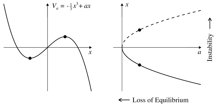
Figure 1.— Fold catastrophe. (Left) Potential $V_{a}(x)=-\frac{1}{3}x^{3}+ax$ for $a=1$. (Right) Equilibrium manifold $x^{2}-a=0$; the stable (unstable) branch is plotted solid (dashed). The two equilibrium positions are marked in both plots.

Catastrophe theory analyzes nonlinear systems that exhibit abrupt changes of behavior, called catastrophes, and are governed, at least locally in the vicinity of the point(s) of change, by a smooth potential function $V_{a}(x)$ that depends upon at least one “behavior” variable (or “active” variable) $x$ and at least one “control parameter” $a$. The force acting on the system in the space of the behavior variable is given by $-\mathrm{d}V_{a}/\mathrm{d}x$, so that the equilibrium positions are given by $\mathrm{d}V_{a}/\mathrm{d}x=0$. Catastrophes occur where these are not simple minima or maxima, but one or more higher derivatives of the potential vanish as well at so-called degenerate critical points. The simplest catastrophe thus occurs for a cubic potential with one control parameter, $V_{a}=-\frac{1}{3}x^{3}+ax$, which has an inflexion point at $x=a=0$. Figure 1 (left panel) illustrates this potential in the domain $a>0$, where it has a minimum (stable equilibrium) at $x=-a^{1/2}$ and a maximum (unstable equilibrium) at $x=a^{1/2}$. The equilibrium branches in the $a$-$x$ plane are plotted in the right panel of Figure 1. As $a$ approaches zero, the two extrema of the potential approach each other and disappear upon merging in the inflexion point of the pure cubic function, which is an end point of the pair of equilibrium branches. The catastrophe occurring at $a=0$ is the fold catastrophe. It occurs by a loss of equilibrium, since both equilibria are lost when the control parameter $a$ is reduced below zero.

From the above it is obvious that every fold catastrophe must be associated with an instability. The two equilibrium branches that join at the catastrophe point are a continuous curve, and the catastrophe point lies at the transition between the stable and unstable parts of the curve, i.e., it is a point of marginal stability. For a system evolving along a sequence of stable equilibria, both $x$ and $a$ may be regarded as parameters of the equilibrium. For the toroidal current channel studied below, the major radius $R$ is a natural choice for the behavior variable, and one of the parameters specifying the external poloidal field $B_{\mathrm{e}}$ is a natural choice for the control parameter, for example, the strength of its sources, $q$, or its decay index $n$. However, it is equally justified to regard $R$ as a parameter describing the geometric properties of the equilibria. One can consider an equilibrium sequence of toroidal current channels of varying $R$, with fixed geometry of the sources of $B_{\mathrm{e}}$, and compute the source strength $q_{\mathrm{eq}}(R)$ giving equilibrium for each $R$. This is equivalent to following the equilibrium curve $a(x)$ in Figure 1 by changing $x$. In this consideration, a loss of equilibrium in the sense of catastrophe theory does not occur, but instability will set in as the degenerate critical point is crossed, resulting in an abrupt transition $x\to\infty$ that is identical to the catastrophe occurring as $a$ is reduced below zero.

In most cases, the problem is not symmetric in $x$ and $a$. Often the derivative $\partial V_{a}/\partial a$ does not represent any physical quantity and is not related to the equilibrium positions of the system. The latter is true in particular in catastrophe theory which considers linear dependencies on the control parameters in the vicinity of the degenerate critical points. Nevertheless, the consideration of instability is not restricted to changes in the control parameters, but analyzes in general how the change of any variable describing the equilibrium affects its stability.

Since both the control parameter $a$ and the behavior variable $x$ change as the system point moves along the stable equilibrium branch toward the point of catastrophe and instability, it is not trivial to distinguish in a remote observation, like in the case of a solar eruption, whether an equilibrium ceases to exist or goes unstable (see also the discussion in Démoulin & Aulanier, 2010). However, by definition, it is a control parameter whose evolution causes the system point to move along the stable equilibrium branch toward the critical point. Typically, this can be the total flux of the external field (Bobra et al., 2008; Su et al., 2011; Savcheva et al., 2012a), the geometry of its sources which sets the height profile of the decay index (Török & Kliem, 2007), its shear whose increase causes a magnetic arcade to expand and eventually collapse, forming a flux rope (Mikic & Linker, 1994), or the twist of a flux rope rooted in a rotating sunspot (Amari et al., 1996; Török & Kliem, 2003; Yan et al., 2012). The observations do not indicate that an external driver typically operates directly at the height of current-carrying flux, although a gradual increase of its footpoint separation may cause the flux to ascend in some cases. In the vicinity of the critical point, a fluctuation of any variable can cause the abrupt change of system behavior.

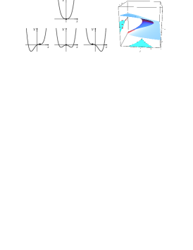
Figure 2.— Cusp catastrophe. (Left four panels) Potential $V_{ab}(x)=\frac{1}{4}x^{4}+\frac{1}{2}ax^{2}+bx$. Top plot: $a=0.6$, $b=0$. Bottom row: $a=-1.2$ and $b=2(-a/3)^{3/2}$, 0, and $-2(-a/3)^{3/2}$ (from left to right). (Right panel) Equilibrium manifold $x^{3}+ax+b=0$. The fold curve, $4a^{3}+27b^{2}=0$, is shown as a red line on the equilibrium manifold and also projected on the $b$–$a$ and $a$–$x$ planes; the enclosed regions of unstable equilibria are colored in cyan. The line $x=b=0$ is added in the $a$–$x$ projection to complete the bifurcation diagram. The same four equilibrium positions are marked in the plots of the potential and bifurcation diagram.

On the other hand, in a numerical simulation one has the freedom to evolve a control parameter (e.g., Chen & Shibata, 2000; Amari et al., 2003; Török & Kliem, 2003; Mackay & van Ballegooijen, 2006; Aulanier et al., 2010; Török et al., 2013) or to change the behavior variable (lifting a flux rope into the torus-unstable height range by a prescribed velocity perturbation, Fan & Gibson, 2007; Kliem et al., 2012). One can of course also test a configuration on any position of the equilibrium manifold for its stability, independent of an evolutionary scenario (e.g., Lionello et al., 1998; Török et al., 2004; Kliem et al., 2013).

The next higher catastrophe arises with a potential $V_{ab}(x)=\frac{1}{4}x^{4}+\frac{1}{2}ax^{2}+bx$. For $a>0$ this potential has one minimum, but for $a<0$ there is a range of the second parameter, $|b|<2(-a/3)^{3/2}$, inside which the potential has two minima enclosing a maximum. Outside this range there is again only one minimum (Figure 2, left four panels). For $a<0$ this maps to the well-known S-shaped equilibrium curve in $b$–$x$ space which has three branches in the range $|b|<2(-a/3)^{3/2}$ and one branch outside (Figure 2, right panel). The nose points of the equilibrium curve correspond to the merging of the maximum of the potential with one of the minima in an inflexion point, i.e., they represent fold catastrophes. Again, these are points of marginal stability, where the unstable branch in the middle part of the S-shaped equilibrium curve smoothly connects to a stable branch. Now, if $a$ increases, approaching zero, the three extrema of the potential approach each other. In $b$–$x$ space this corresponds to a shrinkage of the S-shaped part of the equilibrium curve. The points of fold catastrophe lie on two sections of a curve which approach each other as $a$ increases. As $a\to 0$, all three extrema of the potential and the two sections of the fold curve merge in the point of higher degeneracy, $x=a=b=0$, where the cusp catastrophe occurs. This is a cusp point of the projected fold curve in the $b$–$a$ plane, but the projection in the $a$–$x$ plane shows that the curve is smooth in $b$–$a$–$x$ space. More generally, the equilibrium manifold, the surface given by $x^{3}+ax+b=0$, is everywhere smooth, although it is folded in $\{a<0\}$ (Figure 2, right), since both derivatives $\partial b(x,a)/\partial x$ and $\partial b(x,a)/\partial a$ are everywhere continuous.

With the exception of the cusp point, a loss of equilibrium occurs as the system point crosses the line of fold catastrophes on a path lying in the equilibrium manifold and coming from the stable part of the manifold. At the cusp point, the fold line can be crossed along a smooth path that stays on the equilibrium manifold; coming from the stable side, this must always occur by a change from $a\geq 0$ to $a<0$ along the path. These two facts are perhaps most obvious from the three-dimensional plot of the equilibrium surface and fold curve in Figure 2, but they can also be seen in the $b$–$a$ plane of the control parameters, where they represent crossings of the projected fold curve in opposite directions. Once arrived on the unstable part of the equilibrium manifold after passing through the cusp point, any perturbation will cause the system to rapidly move to one of the neighboring stable equilibrium positions, which is a catastrophe although the move will only be a tiny one in practice, and, of course, is an instability as well. Thus, the cusp catastrophe does not occur by a loss of equilibrium, but by a change of the nature of the equilibrium from stable to unstable. This evolutionary sequence can be termed a loss of stability. The different types of catastrophe are also obvious in the plots of the potential on the left side of Figure 2. A loss of equilibrium occurs in the horizontal transition from the middle panel to and beyond one of the outer panels in the bottom row, and a loss of stability occurs in the downward vertical transition between the middle panels.

Two important aspects must be noted for the relationship between catastrophe and instability. First, instability is part of the cusp catastrophe as this catastrophe occurs by the motion of the system to the unstable part of the equilibrium manifold. Second, the term “loss of stability” is not synonymous with “instability.” Both types of catastrophe—by loss of equilibrium and by loss of stability—are associated with instability. The latter is visualized by the (pitchfork) bifurcation diagram in the $a$–$x$ plane (Figure 2, right): here both the fold and cusp catastrophes occur when the fold line is crossed from the stable to the unstable part of the diagram.

We have seen that the cusp catastrophe occurs at a sub-manifold of the manifold of fold catastrophes, which itself is a sub-manifold of the equilibrium manifold. The dimensionality is reduced by one at each level. This relationship extends to the manifolds of the higher catastrophes, since the degenerate critical points of a certain order are always also degenerate critical points of lower order. Consequently, the fold catastrophe is in general infinite times more likely than any higher catastrophe.

The sample plots of the potential in Figure 2 also show that a catastrophe can occur only by either a loss of equilibrium or a loss of stability. In the first case the minimum disappears as the slope $\mathrm{d}V/\mathrm{d}x$ changes sign only on one side, and in the second case the slope changes sign on both sides simultaneously. In the case of more than one behavior variable, this holds true for each behavior variable and thus in general. Hence, any catastrophe is related to an instability.

For the modeling of solar eruptions, the values of the control parameters can vary in a wide range from event to event. Therefore, only the loss of equilibrium occurring in a fold catastrophe and the associated instability are relevant in practice if the model contains only one behavior variable. The occurrence of a higher catastrophe is a special case, but any eruption mechanism must be able to operate in a wide parameter range. Here it doesn’t matter whether the loss of equilibrium occurs in the potential of the fold catastrophe or in a potential associated with one of the higher catastrophes. Additionally, some of the higher catastrophes, like the cusp catastrophe, do not provide a large change of the system.

If the model includes a second behavior variable, for example the horizontal position of current-carrying flux, which may change in response to asymmetric changes in the photospheric flux distribution, then umbilic catastrophes arise. Lin et al. (2001) demonstrated this for a 2D flux rope equilibrium subject to flux emerging only on one side of the rope. The potentials for the umbilic catastrophes are at least cubic in at least one behavior variable. Therefore, these catastrophes are sub-manifolds of the fold catastrophe for at least one behavior variable (see Poston & Stewart, 1978, Chapters 9.6–9.8 for detail). It thus appears that the fold catastrophe and its associated instability are most relevant in this case as well.

3. Model and basic equations

We consider a self-similarly evolving toroidal current channel of major radius $R$ and minor radius $a$ immersed in a given bipolar or quadrupolar external field as our model for the source region of eruptions. The current channel runs in the center of a toroidal flux rope. Pressure and gravity are neglected, since the Lorentz force dominates in strong active-region fields low in the corona, where most major eruptions arise. While the model appears simplistic at first glance, particularly in apparently missing the solar surface, it does contain all the basic elements needed to describe a catastrophe or instability of flux carrying a net current located above the photospheric boundary: (1) a realistic representation of the external poloidal field in bipolar and simple quadrupolar active regions; (2) the flux rope of a prominence or filament channel; and (3) the oppositely directed image current, given by the lower half of the torus. Also see the discussion of the proper elements to be included in such a model in Lin et al. (2002) and Démoulin & Aulanier (2010) and the support for the presence of net currents from recent investigations of the current distribution in active regions (Ravindra et al., 2011; Georgoulis et al., 2012; Török et al., 2014). We also neglect any external toroidal field components to facilitate an analytical description. The simplicity of the model serves our aim to determine the relation between catastrophe and torus instability. The model yields a transparent expression for the equilibrium manifold, allowing us to consider a number of cases without mathematical complexity, one of them fully analytically.

Essentially the same model was used in the consideration of the torus instability by Osovets (1959) and Kliem & Török (2006), so that we can directly refer to their results. For the purpose of comparing catastrophe and instability, it is necessary that both are described using the same or compatible approximations.

The model in its simplest form lacks photospheric line tying of the flux and implies that the footpoints of the current channel move across the solar surface. We demonstrate below for one of our cases that a simple modeling of the line tying effect can be included and does not change the result in this particular case. The motion of the footpoints across the solar surface hardly affects the threshold of instability, since only infinitesimally small changes of the major radius are considered in determining the threshold. However, the threshold does depend on the shape of the flux rope and on the strength of the external toroidal (shear) field component, with our choice of full toroidal shape (i.e., no line tying) and vanishing external toroidal field giving a relatively low threshold value.

The system is governed by three equations which describe the external equilibrium (i.e., the force balance in the major toroidal direction at the toroidal axis), the internal force-free equilibrium of the current channel (in the direction of the minor radius), and the evolution of the flux enclosed by the torus as the major radius changes.

The external equilibrium of a toroidal current channel in a low-beta plasma is known as the Shafranov, or tokamak, equilibrium (Shafranov, 1966; Bateman, 1978). It is obtained from the following force balance

$$\rho_{m}\frac{\mathrm{d}^{2}R}{\mathrm{d}t^{2}} = \frac{\mu_{0}I^{2}}{4\pi^{2}a^{2}R}\left[\ln\left(\frac{8R}{a}\right)-\frac{3}{2}+\frac{l_{i}}{2}\right]-\frac{IB_{\mathrm{e}}(R)}{\pi a^{2}}$$ (1)

$$= 0\,,$$

where the first term describes the Lorentz self-force of the current (also referred to as the hoop force) and the second term describes the Lorentz force provided by the external poloidal field $B_{\mathrm{e}}(R)$. In the present configuration, the hoop force includes the repulsive force due to the image current. Here $\rho_{m}$ is the mass density in the torus, $I$ is the total ring current, and $l_{\mathrm{i}}$ is the internal inductance per unit length of the ring. $l_{\mathrm{i}}$ is of order unity if the radial profile of the current density is not strongly peaked in the center of the torus, a situation expected to be representative of the flux in solar filament channels, and thus its specific value is only of minor influence on the equilibrium. We adopt the value $l_{\mathrm{i}}=1$ as in Lin et al. (1998, 2002), valid for the linear force-free equilibrium of a current channel (Lundquist, 1951), which is a natural choice for a relaxed force-free equilibrium. The value $l_{\mathrm{i}}=1/2$ for a force-free equilibrium with uniform current density, used in Kliem & Török (2006), yields nearly the same locations of the catastrophe and instability points for the cases considered in Sections 4 and 5, which of course also coincide in each case. The expression in brackets in Equation (1) is exact for large aspect ratio, $R\to\infty$. It remains a good approximation (within 10 percent of the exact value) down to relatively moderate aspect ratios of order $R/a\sim 10$ and deviates from the exact value by up to a factor $\approx 2$ for lower aspect ratios (Žic et al., 2007). The force balance (1) yields an equilibrium current

$$I(R,a)=\frac{4\pi RB_{\mathrm{e}}(R)}{\mu_{0}c_{1}(R/a)}\,,$$ (2)

where $c_{1}(R/a)=\left[\ln(8R/a)-3/2+l_{\mathrm{i}}/2\right]$ has been used as an abbreviation.

The internal equilibrium of the current channel must be close to a force-free field for the low plasma beta characteristic of source regions for solar eruptions ($\beta\sim 10^{-4}\mbox{--}10^{-2}$ in the core of active regions). If a force-free field expands, it remains force free if the expansion is self-similar. Therefore, assuming

$$\frac{R}{a}=\mbox{const}$$ (3)

is a reasonable approximation for the gradual pre-eruptive evolution of a single torus along a sequence of nearly force-free equilibria. This is even more so because the expressions depend on the ratio $R/a$ only logarithmically. Numerical simulations of the torus instability for small plasma beta indicate its initial evolution to be approximately self-similar as well. The assumption of self-similarity implies that the distribution of the current density in the cross section of the current channel remains unchanged; it is thus consistent with the assumption $l_{i}=\mbox{const}$, which has usually been adopted in modeling the evolution toward solar eruptions, and with the relation $aI(R,a)=\mbox{const}$, which has been used in Lin et al. (2002) and other studies of the catastrophe.

It should be kept in mind that self-similarity is not always a good approximation. For the model of a flux rope encircling the Sun considered in Lin et al. (1998), it does not apply as long as the major rope radius is comparable to the solar radius. While the rope expands, its image contracts, which is opposite to self-similar behavior of the system as a whole. This model behaves approximately self-similar when $R\gg R_{\odot}$. Two-dimensional models that place the source of the external field under the current channel, e.g., a line dipole or quadrupole (Forbes & Isenberg, 1991; Isenberg et al., 1993), are similar in this regard.

Finally, the equation governing the evolution of the poloidal flux enclosed by the torus yields an expression for $I(R,a)$. In the solar case, the enclosed poloidal flux has two sources, namely subphotospheric sources of the external poloidal flux and the coronal current that provides the free magnetic energy for the eruption; they are considered to be essentially independent of each other. The sources of the external poloidal flux generally change in strength and geometry on the long time-scale of the gradual pre-eruptive evolution, with the former implying emergence or submergence of flux through the photosphere. The flux in the corona adjusts to these slow changes along a sequence of equilibria, which obey magnetostatic expressions. The sources of the external flux do not change significantly on the short time-scale of the eruption (Schuck, 2010), i.e., during the development of instability. The coronal current generally changes both in the equilibrium sequence and during the eruption, although its subphotospheric roots tend to stay unchanged on the short time-scale of the eruption. The conservation of frozen-in flux on the global scale of the coronal current loop takes dominance over the conditions at its footpoints in constraining the current.

We note that not all of the considerations above carry over to related laboratory plasmas, the details depending on the specific setup. For example, Osovets (1959) considered a pulsed tokamak operation with no external current drive. In this case, the current channel expands and contracts in vacuum, and its current stems solely from induction by the changing external poloidal flux generated in external coils and linked by the torus.

The flux enclosed by the torus is $\Psi=\Psi_{I}+\Psi_{\mathrm{e}}$, where the poloidal flux due to the ring current,

$$\Psi_{I}(R,a)=\mathcal{L}(R,a)I(R,a)\,,$$ (4)

is expressed in terms of the inductance of the torus, $\mathcal{L}(R,a)=\mu_{0}R\left[\ln(8R/a)-2+l_{\mathrm{i}}/2\right]$, and the external poloidal flux is given by

$$\Psi_{\mathrm{e}}(R)=-2\pi\int_{0}^{R}B_{\mathrm{e}}(r)\,r\,\mathrm{d}r\,.$$ (5)

Here we have dropped the common factor $1/2$ referring to the upper half of the enclosed flux (above the photosphere) and extended the integral to $r=R$ instead of the accurate value $r=R-a=R(1-a_{0}/R_{0})$, where $R_{0}$ and $a_{0}$ are the initial values, to be consistent with the treatment in Kliem & Török (2006). This approximation simplifies the resulting algebraic expressions. The neglect of the factor $(1-a_{0}/R_{0})$ causes only small quantitative changes in the large aspect ratio approximation underlying Equation (1). It could easily be incorporated in the resulting expressions, without changing the qualitative results.

The evolution of the enclosed flux during changes of the major torus radius depends on the occurrence of reconnection. We first consider a case in which the field under the current channel has an X-type magnetic configuration. This is a two-dimensional X-point field if the external field is purely poloidal, an X-line in the 3D view of our axisymmetric model. (The X-line becomes a separator field line if an external toroidal field component is present, and it coincides or approximately coincides with a quasi-separator line running within a hyperbolic flux tube if the photospheric boundary is also taken into account, Priest & Démoulin 1995; Titov et al. 2002). Expansion of the current channel in the presence of an X-type structure is likely to be associated with reconnection, both before the eruption (e.g., Aulanier et al., 2010) and during the eruption (e.g., Török & Kliem, 2005). The X-line acts as a seed for the formation of a vertical current sheet and the onset of reconnection. Since the time-scale of reconnection in the corona is shorter than the time-scale of photospheric driving, typically reconnection acts efficiently at the X-line and a large-scale vertical current sheet does not develop in the evolution of a system on the equilibrium manifold (different from the fast evolution during eruption). In the rest of the volume the flux is assumed to be frozen in. Reconnection under the current channel in this non-ideal MHD case adds equal amounts of positive and negative poloidal flux to the area between the current and the photosphere. It also allows the flux rope to “slide through” the external poloidal field: the amount of originally overlying flux transferred by reconnection to the flux rope equals the amount of flux added below the X-line.

Since the flux rope slides through the external field in the non-ideal case, to a first approximation the functional form of $B_{\mathrm{e}}(R)$ remains invariant as the major torus radius changes. This approximation is supported by the agreement of the resulting threshold value with many numerical and observational studies of the torus instability. Gradual changes of the external field can thus be described by changes of the parameters, $p$, in a given function $B_{\mathrm{e}}(R,p)$.

In determining the instability threshold, the parameters of the external field are treated as given. The enclosed flux is then conserved in the non-ideal case,

$$\Psi(R,a) = \mathcal{L}(R,a)I(R,a)+\Psi_{\mathrm{e}}(R)$$ (6)

$$= \Psi_{0}\,,$$

where $\Psi_{0}=\Psi(R_{0},a_{0})$. Here and in the following we use the subscript 0 to denote initial values (of a reference equilibrium at an arbitrary point on the stable part of the equilibrium manifold in parameter space).

As the parameters of the external field $B_{\mathrm{e}}(R,p)$ change in the pre-eruptive evolution considered in the description of catastrophe, both the force $IB_{\mathrm{e}}$ in Equation (1) and the external flux $\Psi_{\mathrm{e}}$ given by Equation (5) change. Including the change $\Delta\Psi_{\mathrm{e}}$ in the equation for the enclosed flux yields

$$\Psi(R,a,p) = \mathcal{L}(R,a)I(R,a)+\Psi_{\mathrm{e}}(R,p)$$ (7)

$$= \Psi_{0}+\Delta\Psi_{\mathrm{e}}(R_{0},p)\,,$$

$$\Delta\Psi_{\mathrm{e}}(R_{0},p) = -2\pi\int_{0}^{R_{0}}[B_{\mathrm{e}}(r,p)-B_{\mathrm{e}}(r,p_{0})]\,r\,\mathrm{d}r\,.$$ (8)

If the sources of the external field change in strength on the Sun, flux must emerge or submerge through the photosphere. This is represented by the term $\Delta\Psi_{\mathrm{e}}$. In our model with toroidal symmetry, where the sources of $B_{\mathrm{e}}$ must be symmetric with respect to the photosphere, this can still be thought of as a gain or loss of flux through the photosphere. On the other hand, if the photospheric flux distribution is rearranged with a fixed strength of its sources, then the change is not associated with emergence or submergence of flux for the frozen-in conditions on the Sun. However, in the parametric representation of geometric changes with fixed functional form $B_{\mathrm{e}}(R,p)$ in the present formulation, the enclosed flux generally changes as $p$ changes. The flux is exchanged between the area enclosed by the torus and the exterior area in this case, not through the photosphere (this is obvious from considering a varying distance of the sources from the plane of the torus). As the torus slides through the external field in response to a change of $B_{\mathrm{e}}$, it regains part or all of the flux exchanged between the two areas. In particular, if the sources of $B_{\mathrm{e}}$ are simply moved along the symmetry axis of the torus, the torus radius can change proportionally to keep equilibrium, and in this case the enclosed external flux stays invariant. Therefore, we choose to use Equation (6) for the enclosed flux if $p$ describes the geometry of the sources of $B_{\mathrm{e}}$, and Equation (7) if $p$ describes their strength. The resulting differences in the location of the catastrophe point remain minor in large parts of parameter space (e.g., in the cases displayed in Figures 4, 6, 7, and 10 below) but they can be considerable for some parameter combinations (the case shown in Figure 9 is an example).

If there is no X-line but rather a bald-patch separatrix surface below the current-carrying flux, then a vertical current sheet cannot immediately form if the current channel expands; it will form only after a considerable expansion has led to sufficient horizontal constriction of the flux below the channel. For thin channels this occurs relatively early (e.g., Forbes & Isenberg, 1991; Lin et al., 2002), so that the remaining evolution on the equilibrium manifold can be described using Equation (6) or (7), but for thick channels this does not occur before the eruption develops strongly (e.g., Gibson & Fan, 2006). In the resulting absence of reconnection in the pre-eruptive evolution, both parts of the enclosed flux are conserved individually, giving us the simple equation for the case of ideal-MHD evolution

$$\Psi_{I}(R,a)=\mathcal{L}(R,a)I(R,a)=\Psi_{I0}\,.$$ (9)

Since the torus cannot “slide through” the external field in ideal MHD, the functional form of $B_{\mathrm{e}}(R)$ must change in this case if the flux rope expands. This generally also includes the formation of currents in the ambient volume.

Topological considerations of active-region evolution suggest that either case can be realized (Titov & Démoulin, 1999). Both possibilities were also supported by data analysis (e.g., Green & Kliem, 2009; Green et al., 2011), active-region modeling (e.g., Su et al., 2011; Savcheva et al., 2012b), and numerical simulation (e.g., Gibson & Fan, 2006; Aulanier et al., 2010).

It is worth noting that Equations (6) and (7) do not describe evolution in a vacuum, although they are based on the assumption that the flux rope moves through the external poloidal field. If the flux rope expanded in vacuum, $\Psi_{I}(R)$ would be conserved (Equation 9), while $\Psi_{\mathrm{e}}(R)$ would change according to Equation (5) with the functional form of $B_{\mathrm{e}}(R,p)$ being preserved exactly. Although the description of the evolving external field as a parameter dependence of $B_{\mathrm{e}}(R,p)$ with fixed functional form still contains an element of vacuum behavior, it represents a reasonable approximation to the MHD behavior of the system, as discussed above in relation to Equation (7).

Moreover, the modeling approach laid out above and also employed in Kliem & Török (2006) should not be categorized as a “circuit model”, since it does not contain any element of an electric circuit. There are no current sources or sinks. Rather the current is a secondary quantity depending on the evolution of the magnetic flux, and given by Equation (1), combined with Equation (6), (7) or (9) which express MHD considerations. Similarly, the assumption made for the internal equilibrium (Equation (3)) expresses a property of a force-free field.

In the following, we consider only the non-ideal case, since a reliable analytical description of the changing function $B_{\mathrm{e}}(R)$ does not yet exist for the ideal-MHD case. Kliem & Török (2006) have formally derived a torus instability threshold $n_{\mathrm{cr}}=2$ in this case, using the parameterized form $B_{\mathrm{e}}(R)=\hat{B}R^{-n}$, where $n$ is not prescribed but determined from the condition of marginal stability; however, they noted that the formulation was not self-consistent. A closer consideration of this case suggests a completely different description, focusing on the Lorentz forces formed in the ambient flux. If the current channel expands self-similarly in the ideal-MHD case, then the frozen-in field component $B_{\mathrm{e}}(R)$ within the channel decreases proportionally to $R^{-2}$. Since $I\propto R^{-1}$ in this case (from Equations (9) and (3)), the external force balance (1) is not affected, i.e., in this approximation no force resisting or amplifying the expansion is induced within the channel. Numerical simulations of this case in the zero-beta limit indicate that the expansion indeed tends to be approximately self-similar (a result of force-freeness). The expansion piles up the ambient flux above the current channel, creating a downward-directed magnetic pressure gradient in the ambient flux. Below the current channel, the flux is stretched upward, reducing the curvature radius of the upward concave field lines, which creates an upward Lorentz force. The global force balance tends to be dominated by the opposing Lorentz forces created in the compressed or stretched ambient flux. Their ratio, and hence the stability of the current channel, again depends on the decay index of the external field, but also quite significantly on the aspect ratio $R_{0}/a_{0}$, with thicker tori being more stable. Numerical simulations indicate a threshold of instability closer to the canonical value of 3/2 for moderate aspect ratio but rising even above 2 for very thick tori; these will be reported in a future study.

The flux equation (7) yields the following expression for the current

$$I(R,a,p)=\frac{\mathcal{L}_{0}I_{0}+\Psi_{\mathrm{e0}}-\Psi_{\mathrm{e}}(R,p)+\Delta\Psi_{\mathrm{e}}(R_{0},p)}{\mathcal{L}(R,a)}\,.$$ (10)

The cases that are instead described by Equation (6) are covered by this expression if the term $\Delta\Psi_{\mathrm{e}}$ is dropped. Inserting Equation (2) into Equation (10) to eliminate the current, and using Equation (3), we obtain the expression for the equilibrium manifold in the non-ideal case,

$$0 = R^{2}B_{\mathrm{e}}(R,p)-R_{0}^{2}B_{\mathrm{e0}}$$ (11)

$$+\frac{c_{1}}{4\pi c_{2}}[\Psi_{\mathrm{e}}(R,p)-\Psi_{\mathrm{e0}}-\Delta\Psi_{\mathrm{e}}(R_{0},p)]\,,$$

where the abbreviation $c_{2}(R/a)=\mathcal{L}(R,a)/(\mu_{0}R)=c_{1}-1/2$ has been introduced. Since the geometry of the flux rope is assumed to be invariant in our model, the expression for the equilibrium manifold shows in a particularly transparent form that the properties of the equilibria are determined by the external field. For the consideration of catastrophe and instability in our model, we do not need to compute the whole field (although it is well known for the specific choices of $B_{\mathrm{e}}(R,p)$ treated below).

To find the point of marginal stability for this model, Kliem & Török (2006) determined at which radius $R$ the force (Equation (1)) resulting from an infinitesimal perturbation of the equilibrium changes sign,

$$\frac{\mathrm{d}}{\mathrm{d}R}\left.\left(\rho_{m}\frac{\mathrm{d}^{2}R}{\mathrm{d}t^{2}}\right)\right|_{R=R_{\mathrm{eq}}}=0\,,$$ (12)

where $R_{\mathrm{eq}}$ is a radius on the equilibrium manifold satisfying $\left.\mathrm{d}^{2}R/\mathrm{d}t^{2}\right|_{R=R_{\mathrm{eq}}}=0$. In their treatment Equations (10) and (3) were inserted in (1), which is equivalent to Equation (11), and then the derivative was taken. The resulting torus instability threshold is

$$n_{\mathrm{cr}}=\frac{3}{2}-\frac{1}{4c_{2}}\,.$$ (13)

This can readily be verified to hold for any smooth function $B_{\mathrm{e}}(R,p)$ by taking the derivative of expression (11) for the equilibrium manifold (which immediately also yields the threshold $n_{\mathrm{cr}}=2$ if the terms proportional to $c_{1}/c_{2}$ are dropped). For aspect ratios in the range typically considered (i.e., $R/a=3\mbox{--}100$), the second term in Equation (13) is a small number in the range 0.05–0.15.

Equation (12) explicitly demonstrates that instability and fold catastrophe are equivalent descriptions of the transition to a non-equilibrium state. At the point of marginal stability, the force resulting from an infinitesimal deviation from equilibrium changes from a restoring to an amplifying force (vanishing derivative of the left-hand side of Equation (1)). This coincides with a degenerate critical point of the underlying potential (vanishing derivative of the expression for the equilibrium manifold in the middle part of Equation (1), as discussed in Section 2), i.e., with a point of catastrophe. Thus any catastrophe occurring in the expansion of the torus in the model considered in this paper must occur at the threshold of torus instability.

This also resolves an apparent problem indicated by the different expressions for the enclosed flux in the description of catastrophe (including the term $\Delta\Psi_{\mathrm{e}}$ in some cases) and instability (excluding the term $\Delta\Psi_{\mathrm{e}}$). Since $\Delta\Psi_{\mathrm{e}}(R_{0},p)$ does not contribute to the derivative of the equilibrium manifold (11), the torus instability threshold (13) is independent of its inclusion, i.e., the two approximations are compatible with each other. Although the position of the degenerate critical point in $R$–$p$ space depends on whether or not $\Delta\Psi_{\mathrm{e}}(R_{0},p)$ is included, it coincides with the instability threshold (13) in either case.

For consistency of the presentation, we will use an aspect ratio $R/a=10$ in all applications that follow, so that the Lorentz self-force of the current channel is well approximated by Shafranov’s expression in Equation (1). It should be noted that the considerations above, in particular the expression (11) for the equilibrium manifold, remain valid for smaller aspect ratio because the inductance, and hence the Lorentz self-force, then still depend on $R$ and $a$ in the same form as Shafranov’s expressions (Žic et al., 2007). Only the definition of the numerical coefficients $c_{1}$ and $c_{2}$ differs.

The relatively high aspect ratio, in combination with the assumption that half of the torus extends above the photosphere, implies a high value of the twist. The field line pitch (the axial length for one winding about the axis) in a force-free current channel is comparable to the radial length-scale of the field, $a$. Therefore, a high twist is unavoidable for high aspect ratio. We disregard the resulting susceptibility of the current channel to helical kinking (Hood & Priest, 1979) and focus exclusively on the stability properties with respect to toroidal expansion (a form of lateral kinking), since it is this instability which is related to the catastrophes investigated previously. A simultaneous consideration of both instabilities in the framework of catastrophe theory (an umbilic catastrophe) has, to our knowledge, not yet been performed. The observations of filaments and prominences indicate that flux ropes in the solar corona typically have a smaller aspect ratio and are stable against the helical kink mode in the majority of cases.

4. Catastrophe versus instability in a bipole field

Figure 3.— Bipolar active-region model (Titov & Démoulin, 1999) showing $B_{z}(x,y)$ in the bottom plane (saturated gray scale), the current channel of major radius $R$ and minor radius $a=0.1R$ as a transparent isosurface of current density, field lines of the force-free field in the current channel, field lines of the purely poloidal field external to the current channel considered in this paper, and the toroidal X-line as a red ring. The bottom plane is positioned at $z\approx 0.2R$. The locations of the peak $|B_{z}|$ values in the bottom plane indicate the positions of the sources of the external poloidal field at $\bm{x}=(\pm L,0,0)$. The major torus radius in this and the subsequent field line plots lies on the stable equilibrium branch close to the catastrophe point.

We first consider a bipole as the source of an external field, with the poles of strength $\pm q$ located at the symmetry axis of the torus at distances $\pm L$ from the torus plane. This is identical to the Titov–Démoulin model of an active region (Titov & Démoulin, 1999), which has been successfully used in qualitative and quantitative numerical modeling of a wide range of solar eruptions (e.g., Török & Kliem, 2005; Schrijver et al., 2008; Kliem et al., 2012). The external field in the torus plane is perpendicular to the plane and given by

$$B_{\mathrm{e}}(R)=\frac{\mu_{0}}{2\pi}\frac{qL}{(R^{2}+L^{2})^{3/2}}\,.$$ (14)

Such a configuration allows us to consider both scenarios for a catastrophe considered previously in the context of solar eruptions, i.e., changing the field amplitude (Forbes & Isenberg, 1991; Isenberg et al., 1993; Lin et al., 1998; Lin & van Ballegooijen, 2002), here parameterized by $q$, and changing the spatial scale of the field (Forbes & Priest, 1995; Lin & van Ballegooijen, 2002), here parameterized by $L$. The catastrophe for this system has already been investigated in Lin et al. (2002), using the more general approximation $aI(R,a)=\mbox{const}$ in place of Equation (3). For comparison with the torus instability threshold, we repeat the analysis here using Equation (3) as in Kliem & Török (2006).

The decay index of the bipole field in the plane of the torus is

$$n_{\mathrm{bp}}=-\frac{d\ln{B_{\mathrm{e}}}}{d\ln{R}}=3(L^{2}/R^{2}+1)^{-1}\,.$$ (15)

The torus instability threshold in the non-ideal MHD case (Equation (13)) lies here at $R/L=[(6c_{2}-1)/(6c_{2}+1)]^{1/2}$, i.e., slightly below unity. In terms of $\xi=R/L$, the expressions required in Equation (11) are

$$R^{2}B_{\mathrm{e}}(R)=\frac{\mu_{0}}{2\pi}\frac{q\xi^{2}}{(\xi^{2}+1)^{3/2}}$$ (16)

and

$$\Psi_{\mathrm{e}}(R)=\mu_{0}q\left[\frac{1}{(\xi^{2}+1)^{1/2}}-1\right]\,.$$ (17)

To see whether and where the torus in the bipole field exhibits catastrophic behavior, we choose a reference equilibrium in the stable part of parameter space, i.e., $R=R_{0}<[(6c_{2}-1)/(6c_{2}+1)]^{1/2}L_{0}$ and $q=q_{0}$, and vary either the bipole strength as $q(t)=\sigma(t)q_{0}$ with fixed geometry $L=L_{0}$, or the geometry as $L(t)=\lambda(t)L_{0}$ with fixed bipole strength $q=q_{0}$. In the former case, the torus must expand to find a new equilibrium if $\sigma$ decreases (which represents flux cancellation under the flux rope or a general decay of an active region). Since $L$ is kept fixed, this implies that the new equilibrium is situated at a radius with a steeper slope for the external field, thus approaching the threshold of the torus instability. If torus instability and catastrophe are equivalent, a catastrophe must then occur. In the latter case, the field strength at the original torus position decreases if $L$ increases (corresponding, for example, to active-region dispersal), so that the torus must also expand to find a new equilibrium. Since the equilibrium manifold depends on $R$ and $L$ only in the combination $\xi=R/L$ (Equations (11), (16), and (17)), $R$ increases proportionally to $L$, representing a simple rescaling of the configuration without approaching a loss of equilibrium or the torus instability threshold (see Lin et al. 2002 and Section 4.2 below).

4.1. Changing the Source Strength

We set $q=\sigma(t)q_{0}$ and $L=L_{0}$. Inserting the expressions (16) and (17) into Equation (11) immediately yields an explicit expression for the equilibrium curve $\sigma=f(R,R_{0}/L,R_{0}/a_{0})$,

$$\sigma=\frac{2\xi_{0}^{2}(\xi_{0}^{2}+1)^{-3/2}}{\begin{array}[]{l}2\xi^{2}(\xi^{2}+1)^{-3/2}\\ \quad{}-(c_{1}/c_{2})[(\xi_{0}^{2}+1)^{-1/2}-(\xi^{2}+1)^{-1/2}]\end{array}}\,.$$ (18)

Here only the denominator depends on $\xi$. It is straightforward to verify that it has a maximum at $\xi=[(6c_{2}-1)/(6c_{2}+1)]^{1/2}$, which is a minimum of the function $\sigma(R)$, i.e., the location of a fold catastrophe point (a nose point of $R(\sigma)$). Inserting this critical radius in expression (15), the decay index of the bipole field at the catastrophe point is found to be $n_{\mathrm{bp}}=3/2-1/(4c_{2})$—exactly the instability threshold given in Equation (13)—, which verifies the correspondence between catastrophe and torus instability of the flux rope. Figure 3 illustrates the equilibrium and Figure 4 plots the function $R(\sigma)$ for $R/a=10$ ($c_{2}=2.88$). The figure also shows a plot of the equilibrium manifold obtained if Equation (6) is used instead of Equation (7). Catastrophe then occurs at the same torus radius (same decay index) but at a somewhat different value of the control parameter.

Figure 4.— Equilibrium torus radius $R/L$ as a function of bipole strength $\sigma$ with the term $\Delta\Psi_{\mathrm{e}}$ in Equation (11) included (thick line) and excluded (thin line) for an aspect ratio of the current channel of $R/a=10$. Solid (dashed) lines represent stable (unstable) equilibria in this and all subsequent plots of the equilibrium manifold.

For comparison, Lin et al. (2002) find a catastrophe occurs at $R/L=0.94$. Using their value for the aspect ratio $R_{0}/a_{0}=100$, our expressions locate the catastrophe/instability point at nearly the same value, $R/L=0.97$. Lin et al. (2002) use the force balance (1) for the external equilibrium, $I\propto a^{-1}$ for the internal equilibrium, and (for this result) the conservation of flux according to Equation (6). The close agreement of the results indicates that the assumption (3), which considerably simplifies the expressions for the equilibrium manifold, is appropriate for our system.

4.2. Changing the Length-scale

Setting $q=q_{0}$ and varying $L(t)=\lambda(t)L_{0}$, Equation (11), with the term $\Delta\Psi_{\mathrm{e}}$ dropped, becomes

$$\frac{2\lambda^{-2}\xi^{2}}{(\lambda^{-2}\xi^{2}+1)^{3/2}}-\frac{c_{1}}{c_{2}}\left[1-\frac{1}{(\lambda^{-2}\xi^{2}+1)^{1/2}}\right]$$ (19)

$$= \frac{2\xi_{0}^{2}}{(\xi_{0}^{2}+1)^{3/2}}-\frac{c_{1}}{c_{2}}\left[1-\frac{1}{(\xi_{0}^{2}+1)^{1/2}}\right]\,,$$

where $\xi=R/L_{0}$ and $\xi_{0}=R_{0}/L_{0}$. One immediately sees that this depends on $\lambda$ and $\xi$ only in the combination $\xi/\lambda$, so that the equilibrium sequence $\xi(\lambda)=\lambda\xi_{0}$ represents a simple rescaling of the configuration, as discussed above and first demonstrated in Lin et al. (2002). Thus, the length-scale $L$ of the bipole is not an appropriate control parameter to obtain catastrophic or unstable behavior of the model.

The simple scaling relationship between $\lambda$ and $\xi$ breaks down if photospheric line tying is included. We have attempted to model this by employing the approximation for the inductance of a line-tied current channel

$$\mathcal{L}(R)=\mu_{0}R\left[\frac{1}{2}\left(\ln\frac{8R}{a_{\mathrm{f}}}+\ln\frac{8R}{a_{\mathrm{a}}}\right)-2+\frac{l_{\mathrm{i}}}{2}\right]$$

developed by Garren & Chen (1994). Here $a_{\mathrm{f}}$ and $a_{\mathrm{a}}$ are the minor torus radii at the footpoints and apex of the current channel, respectively. Setting $a_{\mathrm{f}}=a_{0}$ and using Equation (3) for $a_{\mathrm{a}}$, the above average yields the additive correction $\ln(R/R_{0})/2$ to the logarithmic term in the inductance of a freely expanding torus, which must be applied to the logarithmic term in the force balance (1) as well. The coefficients $c_{1}$ and $c_{2}$ are now functions of $R$ (or $\xi$) but not of $\lambda$. However, since the correction is at most moderate (due to the logarithmic dependence on $R$), since it is applied to both coefficients, and since only the ratio $c_{1}/c_{2}$ enters the equations, the effect on the equilibrium curve $R(\lambda)$ remains very minor, so that a catastrophe still does not occur. This appears quite plausible, since line tying tends to hinder the expansion of the current channel in comparison with free expansion, so that it is more difficult for it to expand into the torus-unstable range as $L(t)/L_{0}$ increases.

5. Catastrophe versus instability in the field of a linear quadrupole

Figure 5.— Quadrupolar active-region model (generalized Titov-Démoulin equilibrium) shown in a format similar to Figure 3. The bottom plane is here positioned at $z=0.1R$ to include the low-lying X-line in the display. The values of the parameters $R/a$, $\kappa$, and $\epsilon$ are identical to Figure 6.

As a second realization of our model we consider the expansion of a torus in the field of a linear quadrupole consisting of two nested bipoles (denoted by subscripts 1 and 2); both are placed symmetrically with respect to the torus plane at the symmetry axis of the torus. This field can have a steeper slope than that of a single bipole, especially below a magnetic null line (X-line), which is present for a wide range of parameter combinations $(q_{2}/q_{1},L_{2}/L_{1})$ if the two bipoles are oppositely directed (see Figure 5 for an illustration). Thus, torus instability tends to occur at a smaller $R$, and the catastrophe has also been found to occur at a small height above the photosphere if the external field is quadrupolar (Isenberg et al., 1993). All configurations considered below include an X-line above and a second X-line below the current channel for parameters in the vicinity of the catastrophe point, except the configuration in Figures 8 and 9.

The external field in the torus plane is given by

$$B_{\mathrm{e}}(R) = \frac{\mu_{0}}{2\pi}\left[\frac{q_{1}L_{1}}{(R^{2}+L_{1}^{2})^{3/2})}+\frac{q_{2}L_{2}}{(R^{2}+L_{2}^{2})^{3/2})}\right]$$ (20)

$$= \frac{\mu_{0}}{2\pi}\frac{q_{1}}{L_{1}^{2}}\left[\frac{1}{(\xi^{2}+1)^{3/2}}+\frac{\epsilon\kappa^{-2}}{(\xi^{2}\kappa^{-2}+1)^{3/2}}\right],$$

where now $\xi=R/L_{1}$ and $\epsilon=q_{2}/q_{1}$, $\kappa=L_{2}/L_{1}$. It has a decay index

$$n_{\mathrm{qp}}=3\xi^{2}\frac{(\xi^{2}+1)^{-5/2}+\epsilon\kappa^{-4}(\xi^{2}\kappa^{-2}+1)^{-5/2}}{(\xi^{2}+1)^{-3/2}+\epsilon\kappa^{-2}(\xi^{2}\kappa^{-2}+1)^{-3/2}}\,.$$ (21)

This cannot be analytically solved for $\xi$ to obtain the threshold radii corresponding to the critical decay index value (13). The expressions for $R^{2}B_{\mathrm{e}}(R)$ and $\Psi_{\mathrm{e}}(R)$ are fully analogous to (16) and (17), with obvious extensions for the second pair of sources in the linear quadrupole.

If the field strength or length-scale of the quadrupole are varied with constant ratios $\epsilon$ and $\kappa$, then one expects the system to behave in a similar manner with regard to the catastrophe as in the case of the bipole field. This is verified below. Additionally, we consider changes of $\epsilon$ or $\kappa$ leading to catastrophe.

5.1. Changing the Source Strength

Figure 6.— Equilibrium torus radius $R/L_{1}$ as a function of quadrupole strength $\sigma$ for an aspect ratio of $R/a=10$, size ratio $\kappa=2$, and charge ratio $\epsilon=-1$.

First we consider a proportional decrease of all four sources in the linear quadrupole, $q_{1}(t)=\sigma(t)q_{10}$, $\epsilon=\mbox{const}$, $L_{1}=L_{10}$, $\kappa=\mbox{const}$. Inserting the expressions for $B_{\mathrm{e}}(R)$ and $\Psi_{\mathrm{e}}(R)$ into Equation (11) again yields an explicit expression for the equilibrium curve $\sigma=f(R,R_{0}/L_{1},R/a,\epsilon,\kappa)$,

$$\sigma=\frac{2\xi_{0}^{2}[(\xi_{0}^{2}+1)^{-3/2}+\epsilon\kappa^{-2}(\xi_{0}^{2}\kappa^{-2}+1)^{-3/2}]}{\begin{array}[]{l}2\xi^{2}[(\xi^{2}+1)^{-3/2}+\epsilon\kappa^{-2}(\xi^{2}\kappa^{-2}+1)^{-3/2}]\\ \quad{}-(c_{1}/c_{2})[(\xi_{0}^{2}+1)^{-1/2}-(\xi^{2}+1)^{-1/2}\\ \quad{}+\epsilon(\xi_{0}^{2}\kappa^{-2}+1)^{-1/2}-\epsilon(\xi^{2}\kappa^{-2}+1)^{-1/2}]\end{array}}\,,$$ (22)

but a closed analytical expression for the maximum of the denominator can here no longer be obtained. The plot of this expression in Figure 6, for the same value of the aspect ratio as in Figure 4 and for $\kappa=2$, $\epsilon=-1$, demonstrates the expected fold catastrophe at $(\sigma,R/L_{1})=(0.2738,0.7059)$, i.e., at a smaller radius than for the external bipole field. At this radial position the field of the linear quadrupole has a decay index of $n_{\mathrm{qp}}=1.413$, exactly the threshold (13) of torus instability for the chosen aspect ratio and $l_{i}$.

Another path to catastrophe consists in varying the strength of only one pair of sources in the quadrupole. We first let the relative strength of the outer source pair increase as $\epsilon(t)=\delta(t)\epsilon_{0}$ for opposite polarity ($\epsilon<0$), which decreases the external field in the torus plane as well. The current channel is thus forced to find new equilibrium positions at larger $R$ where $n_{\mathrm{qp}}$ is higher. Equation (11) can again be easily solved for $\delta=f(R,R_{0}/L_{1},R/a,\epsilon,\kappa)$. The resulting expression

$$\delta=\frac{\begin{array}[]{l}2\xi_{0}^{2}[(\xi_{0}^{2}+1)^{-3/2}+\epsilon_{0}\kappa^{-2}(\xi_{0}^{2}\kappa^{-2}+1)^{-3/2}]\\ ~{}{}-2\xi^{2}(\xi^{2}+1)^{-3/2}\\ ~{}{}+(c_{1}/c_{2})[(\xi_{0}^{2}+1)^{-1/2}-(\xi^{2}+1)^{-1/2}]\end{array}}{\begin{array}[]{l}2\epsilon_{0}\xi^{2}\kappa^{-2}(\xi^{2}\kappa^{-2}+1)^{-3/2}]\\ ~{}{}-\epsilon_{0}(c_{1}/c_{2})[(\xi_{0}^{2}\kappa^{-2}+1)^{-1/2}-(\xi^{2}\kappa^{-2}+1)^{-1/2}]\end{array}}$$ (23)

is similar in structure to (22) and also requires a numerical evaluation to demonstrate the catastrophe. Using $\kappa=2$ and $\epsilon=-1$ as in Figure 6, the catastrophe point is found at $(\delta,R/L_{1})=(1.846,0.5396)$ where $n_{\mathrm{qp}}=1.413$, again exactly at the threshold of the torus instability (see Figure 7). It lies in the radial range of steeply increasing decay index below the magnetic null point at $R/L_{1}=1.2$.

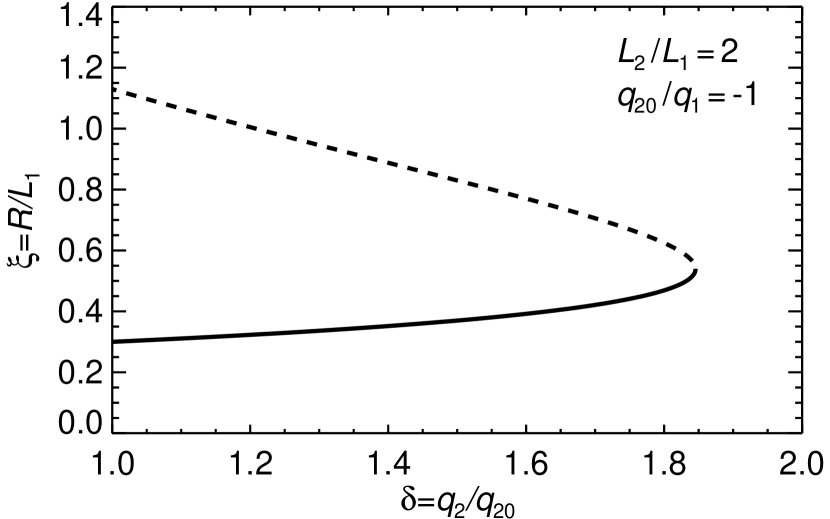
Figure 7.— Equilibrium torus radius $R/L_{1}$ as a function of relative strength of the source pairs in the linear quadrupole, measured by $\delta=\epsilon/\epsilon_{0}=q_{2}/q_{20}$, with the outer pair increasing in strength and otherwise the same parameters as in Figure 6.

Figure 8.— Quadrupolar active-region model (generalized Titov-Démoulin equilibrium) shown in a format similar to Figure 3 for values of $R/a$ and $\kappa$ as in Figure 9.

Figure 9.— Equilibrium torus radius $R/L_{1}$ as a function of relative strength of the source pairs in the linear quadrupole, with the inner pair increasing in strength, size ratio $\kappa=1/3$, and aspect ratio $R/a=10$.

By placing the second bipole inside the first, $\kappa<1$, and considering relatively small ratios of their source strengths, $|\epsilon|=|q_{2}/q_{1}|<1$, we can address the influence of flux emergence on the equilibrium, a process thought to be an efficient trigger of eruptions (Feynman & Martin, 1995). Although the dynamical behavior caused by reconnection between emerging and preexisting flux is likely to play an important role in the triggering (e.g., Archontis & Hood, 2012; Kusano et al., 2012), the effects of the new flux on the force balance of the current channel and on the decay index profile $n_{\mathrm{qp}}(R)$ alone can facilitate the transition to eruptive behavior. Figures 8 and 9 show this for flux emerging with an orientation anti-parallel to the main flux in the region, $\epsilon_{0}=-0.1$, and $\kappa=1/3$. This configuration contains two X-lines which do not lie in the plane of the torus. Equations (7), (8), (11), and thus (23) apply here as well, since reconnection will occur at the X-lines as the torus expands, allowing it to “slide through” the external poloidal field without changing the amount of enclosed flux. Reconnected external flux is here transferred into the side lobes under the X-lines instead of being added under the current channel. The increase of the enclosed flux due to the emergence, which drives the expansion of the torus, is described by the term $\Delta\Psi_{\mathrm{e}}$ in Equation (7). The torus radius before flux emergence ($R/L_{1}\approx 0.47$ for $\delta\to 0$) lies on the stable part of the equilibrium manifold (compare with Figure 4). The emergence of anti-parallel flux weakens the external poloidal field at the position of the current channel (involving reconnection in the corona), so that the channel expands to find a new equilibrium. Since now the profile $B_{\mathrm{ep}}(R)$ is flatter in the range around the original position $R_{0}$, a catastrophe occurs at a larger radius than in Figure 4, $(\delta,R/L_{1})=(5.603,1.283)$, but again exactly at the threshold of torus instability: at this point $n_{\mathrm{qp}}=1.413$.

We did not find a catastrophe for $\kappa<1$ and $\epsilon$ increasing from zero (modeling the emergence of flux with a parallel orientation). An occurrence of catastrophe in this part of parameter space requires the positive $\epsilon$ to decrease to a small value, which weakens the external poloidal field in the plane of the torus, as in all other cases considered in this paper. For completeness we note that catastrophe and instability can be found for $\epsilon$ increasing from zero if the term $\Delta\Psi_{\mathrm{e}}$ is dropped in expression (7) for the enclosed flux. This changes the relationship $I(R,p)$ and thus the balance between the hoop force (quadratic in $I$) and the retracting force (linear in $I$) in Equation (1), allowing the torus to expand in a range of increasing small positive $\epsilon$ values. Since the new flux is of smaller spatial scale, it raises the decay index and the expansion leads to catastrophe, again at the threshold of torus instability.

5.2. Changing the Length-scale

Figure 10.— Equilibrium torus radius $R/L_{1}$ as a function of the size ratio of the outer and inner source pairs in the linear quadrupole, measured by $\nu=\kappa/\kappa_{0}=L_{2}/L_{20}$, for the same parameters as in Figure 6. Excluding (including) the term $\Delta\Psi_{\mathrm{e}}$ in Equation (11) yields the equilibria on the thick (thin) line.

A proportional change of both length-scales in the linear quadrupole, $L_{1}(t)=\lambda(t)L_{10}$ with $\kappa=\mbox{const}$, has the same effect as scaling the length-scale of the bipole field. The equilibrium radius of the current channel changes proportionally to $\lambda(t)$ if the term $\Delta\Psi_{\mathrm{e}}$ is dropped, and neither instability nor catastrophe are reached in this case (Equation (11), evaluated for this equilibrium, again depends on $R/R_{0}$ and $\lambda$ only in the combination $R/(\lambda R_{0})$).

We thus consider the evolution driven by changing the size ratio of the bipoles, $\kappa(t)=\nu(t)\kappa_{0}$, with all other parameters held fixed, corresponding to a rearrangement of the flux distribution in the photosphere. Similar to the increase of $|\epsilon|$ in Figures 7 and 9, an approach of $L_{1}$ and $L_{2}$ reduces the external field at the position of the current channel. We show this for a decrease of $\kappa$ from the value used in Figures 6 and 7. The equilibrium manifold (Equation (11) with the term $\Delta\Psi_{\mathrm{e}}$ dropped) is given by

$$2\xi^{2}[(\xi^{2}+1)^{-3/2}+\epsilon(\nu\kappa_{0})^{-2}(\xi^{2}(\nu\kappa_{0})^{-2}+1)^{-3/2}]$$

$${}-(c_{1}/c_{2})[1+\epsilon-(\xi^{2}+1)^{-1/2}-\epsilon(\xi^{2}(\nu\kappa_{0})^{-2}+1)^{-1/2}]$$

$$=2\xi_{0}^{2}[(\xi_{0}^{2}+1)^{-3/2}+\epsilon\kappa_{0}^{-2}(\xi_{0}^{2}\kappa_{0}^{-2}+1)^{-3/2}]$$

$$\phantom{=}{}-(c_{1}/c_{2})[1+\epsilon-(\xi_{0}^{2}+1)^{-1/2}-\epsilon(\xi_{0}^{2}\kappa_{0}^{-2}+1)^{-1/2}]\,.$$

(24)

This implicit equation in both $\xi=R/L_{1}$ and $\nu$ must be evaluated numerically. The result, plotted in Figure 10, exhibits a fold catastrophe at $(\nu,R/L_{1})=(0.5710,0.5630)$ where $n_{\mathrm{qp}}=1.413$, exactly at the threshold of torus instability.

6. Summary and Conclusion

Using a toroidal flux rope embedded in a bipolar or quadrupolar external field as a model for current-carrying coronal flux and its associated image current, we have demonstrated the occurrence of fold catastrophe by loss of equilibrium when magnetic reconnection can proceed at an X-line under the flux rope. Several evolutionary scenarios have been considered, which include changing the source strength and length-scale of the external field. In each case, the critical point for occurrence of the catastrophe coincides exactly with the threshold for torus instability if the same or compatible approximations are used, a result demonstrated to hold in general for the adopted model. Catastrophe and torus instability are thus equivalent descriptions for the onset of an eruption. They are based on the same force balance for equilibrium and produce an onset of eruption at the same point.

Thus, the merits of each description can be exploited while one can be sure that the other description will yield the same onset point of eruption. Analyzing an equilibrium for the occurrence of catastrophe always includes a model for the pre-eruptive evolution and avoids the consideration of unstable equilibria far away from the critical point, which may be impossible to reach in reality. Analyzing the stability of an equilibrium localizes the critical point without the need to model the pre-eruptive evolution and in a formulation independent of the specifics of such a model. Moreover, since only infinitesimally small changes of the parameters must be considered in a stability analysis, the adopted approximations may be better satisfied than during the whole modeled pre-eruptive evolution in an analysis of catastrophe. It is clear, however, that the approximations are equally satisfied in the vicinity of the critical point.

References

- Amari et al. (2003) Amari, T., Luciani, J. F., Aly, J. J., Mikic, Z., & Linker, J. 2003, ApJ, 595, 1231
- Amari et al. (1996) Amari, T., Luciani, J. F., Aly, J. J., & Tagger, M. 1996, ApJ, 466, L39
- Antiochos et al. (1999) Antiochos, S. K., DeVore, C. R., & Klimchuk, J. A. 1999, ApJ, 510, 485
- Archontis & Hood (2012) Archontis, V., & Hood, A. W. 2012, A&A, 537, A62
- Aulanier et al. (2010) Aulanier, G., Török, T., Démoulin, P., & DeLuca, E. E. 2010, ApJ, 708, 314
- Bateman (1978) Bateman, G. 1978, MHD Instabilities (MIT Press, Cambridge, MA)
- Bobra et al. (2008) Bobra, M. G., van Ballegooijen, A. A., & DeLuca, E. E. 2008, ApJ, 672, 1209
- Chen & Shibata (2000) Chen, P. F., & Shibata, K. 2000, ApJ, 545, 524