Interpreting the sub-linear Kennicutt-Schmidt relationship: The case for diffuse molecular gas

Abstract

Recent statistical analysis of two extragalactic observational surveys strongly indicate a sublinear Kennicutt-Schmidt (KS) relationship between the star formation rate ($\Sigma_{\rm SFR}$) and molecular gas surface density ($\Sigma_{\rm mol}$). Here, we consider the consequences of these results in the context of common assumptions, as well as observational support for a linear relationship between $\Sigma_{\rm SFR}$ and the surface density of dense gas. If the CO traced gas depletion time ($\tau_{\rm dep}^{\rm CO}$) is constant, and if CO only traces star forming giant molecular clouds (GMCs), then the physical properties of each GMC must vary, such as the volume densities or star formation rates. Another possibility is that the conversion between CO luminosity and $\Sigma_{\rm mol}$, the $X_{\rm CO}$ factor, differs from cloud-to-cloud. A more straightforward explanation is that CO permeates the hierarchical ISM, including the filaments and lower density regions within which GMCs are embedded. A number of independent observational results support this description, with the diffuse gas comprising at least 30% of the total molecular content. The CO bright diffuse gas can explain the sublinear KS relationship, and consequently leads to an increasing $\tau_{\rm dep}^{\rm CO}$ with $\Sigma_{\rm mol}$. If $\Sigma_{\rm SFR}$ linearly correlates with the dense gas surface density, a sublinear KS relationship indicates that the fraction of diffuse gas $f_{\rm diff}$ grows with $\Sigma_{\rm mol}$. In galaxies where $\Sigma_{\rm mol}$ falls towards the outer disk, this description suggests that $f_{\rm diff}$ also decreases radially.

1 Introduction

As observations reveal that stars form predominantly in the molecular component of the interstellar medium (ISM), the physical conditions of the H₂ gas undoubtedly influence the star formation process. For example, the star formation rate (SFR) is directly related to the amount of molecular gas. This fundamental property is supported by observations, often through the detection of the CO ($J=1-0$) rotational line as a molecular gas tracer, and some combination of stellar UV, H$\alpha$ from HII regions, and dust thermal emission in the infrared (IR) due to heating from young stars (e.g Kennicutt & Evans, 2012, and references therein). Though the trend of increasing SFR with higher CO luminosity is unambiguous, quantifying such correlations, as well as the associated theoretical interpretations (Mac Low & Klessen, 2004; McKee & Ostriker, 2007), remain a subject of considerable debate.

One formulation of the correlation between the surface densities of the star formation rate $\Sigma_{\rm SFR}$ and molecular gas $\Sigma_{\rm mol}$ is the power-law “Kennicutt-Schmidt” (hereafter KS, Schmidt, 1959; Kennicutt, 1989) relationship:

$$\Sigma_{\rm SFR}=a\Sigma_{\rm mol}^{N_{\rm mol}}.$$ (1)

The surface densities in Equation 1 are estimated by employing conversion factors, such as the $X_{\rm CO}$ factor for translating the CO luminosity to $\Sigma_{\rm mol}$ (see Bolatto et al., 2013, and references therein), and an appropriate factor for estimating $\Sigma_{\rm SFR}$ from the star formation tracer (see references in Kennicutt & Evans, 2012). The correlation between $\Sigma_{\rm SFR}$ and the total gas surface density, including the contribution of HI, exhibits larger scatter (Bigiel et al., 2008; Schruba et al., 2011) further indicative of a more direct link between star formation and the molecular component.

Estimates of the KS parameters $a$ and the index $N_{\rm mol}$ in Equation 1 range from super-linear ($\sim$1.5, Kennicutt, 1989; Liu et al., 2011; Momose et al., 2013), linear (Bigiel et al., 2008; Leroy et al., 2013), to sublinear (Shetty et al. 2013, hereafter SKB13, and Shetty et al. 2014). Kennicutt (1989, 1998) measured an index $\approx 1.4\,\pm$ 0.15 from unresolved observations over entire galactic disks, covering a range over five orders of magnitude in gas surface density. These observations included both normal spirals as well as IR starbursts, and considered the total HI + H₂ gas surface densities. One interpretation for a KS index of $\sim$1.5 is that the primary mechanism in the star formation process is the free fall collapse of molecular clouds (Elmegreen, 1994; Kennicutt, 1998). For a recent review of explanations of the KS relationship, see Dobbs et al. (2013).

However, recent resolved extragalactic observations on 100 $-$ 1000 pc scales demonstrated a tighter molecular KS relationship with lower indices. The analysis of the STING and HERACLES surveys advocated for a linear KS relationship, with significant variations between galaxies (Leroy et al., 2008, 2009, 2013; Bigiel et al., 2008; Schruba et al., 2011; Rahman et al., 2011, 2012). The interpretation of a linear KS relationship is that CO is primarily tracing star forming clouds with relatively uniform properties, including $\Sigma_{\rm SFR}$. A direct consequence of this description is that the depletion time of the CO traced gas is constant and approximately 2 Gyr, both within and between galaxies. Evidently, there is no consensus on either the precise KS parameter estimates, or the associated interpretation.

Two recent statistical analyses of STING and a sub-sample of HERACLES by SKB13 and Shetty et al. (2014) have indicated that the data actually favor a sublinear KS relationship for both ensembles, as well as for most of the individual galaxies. Those works developed and applied a Bayesian fitting method that included a treatment of uncertainties, and provides parameter estimates for each individual galaxy as well as the population. SKB13 explained the advantages of a hierarchical Bayesian method for fitting the KS relationship, and demonstrated its accuracy over common non-hierarchical methods (see also Kelly, 2007; Gelman & Hill, 2007; Kruschke, 2011; Gelman et al., 2004).

Other recent efforts favor a sublinear KS relationship as well. Using H$\alpha$ observations of M51 at 170 pc scales, Blanc et al. (2009) infer a sublinear KS relationship, $N_{\rm mol}$ $=$ 0.82 $\pm$ 0.05. Additionally, Ford et al. (2013) estimate $N_{\rm mol}$ $\approx$ 0.6 in M31 from observations at a comparable scale. Finally, Wilson et al. (2012) find that the ratio of integrated CO ($J=3-2$) to IR luminosity increases with CO ($J=3-2$) luminosity (see their Fig. 5), suggesting $N_{\rm mol}$ $<$ 1. How can we interpret this emerging evidence for the sublinear KS relationship?

The standard interpretation is that CO ($J=1-0$) traces “clouds” or “giant molecular clouds” (GMCs, e.g. Dickman et al., 1986; Solomon et al., 1987). Several theories have attempted to explain the index of the KS relationship, assuming that GMCs constitute the basic star forming unit, and that these GMCs are “virialized” (e.g. Krumholz & McKee, 2005). These assumptions, however, face difficulty if the CO line is not solely a cloud tracer, but rather also delineates more diffuse molecular gas distinguishable from the densest star forming regions.

SKB13 attribute the sublinear KS relationship to the presence of CO outside of star forming regions, perhaps in a diffuse but pervasive molecular component. This description is consistent with a complex, hierarchical ISM consisting of shells, filaments, low density ephemeral wisps, besides the well-known high density star forming clouds. In this work, we explore this further and consider how and/or to what extent common assumptions about GMCs can withstand a sublinear KS relationship.

In the next section, we discuss gas depletion times. Then, in Section 3 we provide three explanations for a sublinear KS relationship, including the presence of the diffuse molecular component and its role in estimating star formation efficiencies. Subsequently, in Section 4 we describe independent observational investigations revealing diffuse molecular gas. We then provide a description of this component in the hierarchical ISM in Section 5, and additional associated implications in Section 6. We conclude with a summary in Section 7.

2 Implications of a sublinear KS relationship

A corollary of a sublinear KS relationship is that the gas depletion time,

$$\tau_{\rm dep}^{\rm CO}=\Sigma_{\rm mol}/\Sigma_{\rm SFR},$$ (2)

increases with increasing gas surface density. As evident in Figure 2 in Shetty et al. (2014), a number of galaxies portray this trend, with only a few galaxies in the STING and Bigiel et al. (2008) surveys being consistent with a constant $\tau_{\rm dep}^{\rm CO}$.

Figure 1 shows estimates of the depletion time and surface density of M51, estimated from BIMA SONG CO observations (Helfer et al., 2003), FUV Nearby Galaxy Survey (NGS; Gil de Paz et al., 2007) and the Spitzer SINGS survey (Kennicutt et al., 2003). The points show $\Sigma_{\rm mol}$, which is the product of the observed luminosities and the standard $X_{\rm CO}$ factor, and $\tau_{\rm dep}^{\rm CO}$ obtained through Equation (2). The dashed line marks a constant $\tau_{\rm dep}^{\rm CO}$ = 2 Gyr. Clearly, $\tau_{\rm dep}^{\rm CO}$ increases with $\Sigma_{\rm mol}$.

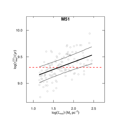
Figure 1: Molecular gas depletion times $\tau_{\rm dep}^{\rm CO}$ and surface densities $\Sigma_{\rm mol}$ in M51. Grey points are the $\tau_{\rm dep}^{\rm CO}$ and $\Sigma_{\rm mol}$ estimated from the observations (and publically available in Bigiel et al., 2010). Thick and thin lines mark the median and $2\sigma$ range of the linear regression from SKB13. Dashed line marks a constant $\tau_{\rm dep}^{\rm CO}$ = 2 Gyr.

The thick solid line in Figure 1 is the predicted trend for $N_{\rm mol}$ = 0.72, which is the most likely value from the hierarchical Bayesian fit from SKB13. The thin solid lines indicate the range of plausible KS fits at 95% confidence from SKB13. Table 1 lists the 2.5%, 50%, and 97.5% quantiles of $\tau_{\rm dep}^{\rm CO}$ at five different values of $\Sigma_{\rm mol}$. The most likely value of $\tau_{\rm dep}^{\rm CO}$ increases from 1.7 Gyr at 25 M_⊙ pc^-2 to 3 Gyr at 200 M_⊙ pc^-2.

Table 1: Estimated Depletion Times in M51

$\Sigma_{\rm mol}$	$\tau_{\rm dep}^{\rm CO}$ (2.5%)	$\tau_{\rm dep}^{\rm CO}$(50%)	$\tau_{\rm dep}^{\rm CO}$(97.5%)
(M⊙ pc-2)	(Gyr)	(Gyr)	(Gyr)
25	1.2	1.7	2.4
50	1.5	2.1	2.9
100	1.8	2.5	3.5
150	2.0	2.8	4.0
200	2.2	3.1	4.4

The inverse of $\tau_{\rm dep}^{\rm CO}$ is the rate of star formation per unit surface density, often referred to as the star formation “efficiency” $\epsilon_{\rm mol}^{\rm CO}$ per unit time. This rate corresponds to the fraction of CO traced gas converted into stars over some timescale. Figure 1 indicates that there are some fundamental differences in the star formation properties as the gas surface densities varies.

3 Origins of a sub-linear KS Relationship

In this section, we consider three possible explanations for the inferred sublinear KS relationship. The first two are systematic effects that produce the observed trends when the underlying KS relationship is linear. In these subsections, we explore the possibility that the inferred variable and sublinear relationship arises due to variations in cloud properties and the $X_{\rm CO}$ factor. However, given the wide range in KS slopes, these scenarios are unlikely. The third interpretation is that CO is also tracing significant amounts of diffuse molecular gas.

3.1 Clouds with different properties?

A popular explanation for a linear KS relationship is that the observed CO luminosity is directly proportional to the number of star-forming clouds or GMCs, with all clouds having similar properties, such as the volume density, the efficiency of the cloud, and the star formation rate. In observations with 100 $-$ 1000 pc resolutions, the individual clouds are not resolved, but rather their CO flux is dispersed throughout the beam. Under this assumption, regions with more clouds emit more CO, in proportion to the number of clouds. Extragalactic CO observations, therefore, are simply “counting clouds”.

However, the sublinear KS relationship suggest that the clouds do not have the same properties, so there is no one-to-one correspondence between the CO luminosity and the number of clouds in the beam. Two likely possibilities are that the star formation efficiencies vary, and/or that the volume densities of the clouds are not constant.

For instance, if the properties of star-forming clouds are highly sensitive to the effects of feedback, then the efficiency would depend on the evolutionary state of the cloud. Younger clouds, which have yet to form (many) stars, are unaffected by feedback. As the cloud evolves, feedback processes from within begin to dramatically alter the cloud, until it is eventually destroyed. Supporting this description, Murray (2011) and Battisti & Heyer (2014) infer a wide range of efficiencies (per free-fall time), and dense gas fractions, respectively, spanning over an order of magnitude (see also Murray & Rahman, 2010). These results suggest that individual clouds could have a time-dependent efficiencies. The systematic trend of a decreasing $\epsilon_{\rm mol}^{\rm CO}$ with increasing $\Sigma_{\rm mol}$ (Fig. 1) could be indicative of a decreasing efficiency with increasing GMC mass, if CO is indeed only tracing star-forming clouds.

Another closely related possibility is that the volume density differs between clouds. Such differences may also lead to a variable efficiencies. Quantifying the densities of clouds requires knowledge of the cloud masses and sizes. As the clouds are unresolved to begin with, it is not possible to do so with the CO observations alone.

3.2 Variations in the $X_{\rm CO}$ factor?

The measured values of $\Sigma_{\rm mol}$ depend on the assumptions in translating the CO brightness to gas densities. Most studies to date employ the standard Galactic value $X_{\rm CO}$ = 2$\times 10^{20}$ cm^-2 K^-1 km^-1 s to convert the observed intensity $W_{\rm CO}$ to H₂ column densities. As $\Sigma_{\rm mol}$ is a surface density,

$$\Sigma_{\rm mol}\propto X_{\rm CO}W_{\rm CO}.$$ (3)

For an assumed constant $X_{\rm CO}$, Equation 1 simply states:

$$\Sigma_{\rm SFR}\propto W_{\rm CO}^{N_{\rm mol}}.$$ (4)

If $\Sigma_{\rm SFR}\propto\Sigma_{\rm mol}$,

$$\Sigma_{\rm SFR}\propto X_{\rm CO}W_{\rm CO}.$$ (5)

If the estimated value of $N_{\rm mol}$ is not unity, $X_{\rm CO}$ would have to vary with $W_{\rm CO}$. Let us consider the relation:

$$X_{\rm CO}\propto W_{\rm CO}^{\beta}.$$ (6)

Together, Equations (4) - (6) require that

$$\beta=N_{\rm mol}-1.$$ (7)

If the $\tau_{\rm dep}^{\rm CO}$ = 2 Gyr, then we could solve

$$X_{\rm CO}\propto\frac{(2\times 10^{9}\,{\rm yr}^{-1})\,\Sigma_{\rm SFR}}{W_{\rm CO}}.$$ (8)

Figure 2 shows the $X_{\rm CO}$ $-$ $W_{\rm CO}$ relationship required to produce a contant $\tau_{\rm dep}^{\rm CO}$ = 2 Gyr for M51. We find that $X_{\rm CO}$ varies in the range 19.8  $\buildrel<\over{\sim}$  log($X_{\rm CO}$/[cm^-2 K^-1 km^-1 s])  $\buildrel<\over{\sim}$  20.8 cm^-2 K^-1 km^-1 s. The line shows a linear regression fit to the data, with slope $\beta=-0.3$, which suggests a steeper $X_{\rm CO}$ $-$ $W_{\rm CO}$ dependence compared to results relying on the assumption of virial equilibrium (Solomon et al., 1987). This slope can be directly estimated from Equation 7 with $N_{\rm mol}$ = 0.7, which is the most likely estimated KS slope for M51 (SKB13).

Figure 2: The variation of the conversion factor $X_{\rm CO}$ with CO intensity $W_{\rm CO}$ required for $\tau_{\rm dep}^{\rm CO}$ = 2 Gyr. The line shows the linear regression result, which has a slope of $-$0.3, [consistent with $N_{\rm mol}$ = 0.7, see Equations (5)-(7)].

As indicated by Equation (7), in order for $\tau_{\rm dep}^{\rm CO}$ to be constant, there should be an inverse correlation between $X_{\rm CO}$ and $W_{\rm CO}$ if $N_{\rm mol}$ $<$ 1. The precise value of $\beta$ depends on the magnitude of the sublinearity, and therefore the properties of the individual galaxies. Indeed, theoretical and observational efforts have clearly demonstrated that $X_{\rm CO}$ differs in environments with a range of metallicities, radiation fields, and/or turbulence levels (e.g. van Dishoeck & Black, 1988; Maloney & Black, 1988; Rubio et al., 2004; Glover & Mac Low, 2011; Leroy et al., 2011; Ostriker & Shetty, 2011; Shetty et al., 2011a; Narayanan et al., 2011, 2012; Sandstrom et al., 2013; Lee et al., 2014). However, many galaxies in the STING and HERACLES sub-samples investigated by SKB13 and Shetty et al. (2014) are local universe star-forming galaxies, and are therefore believed to have similar (solar) metallicities and turbulence levels. In order to recover an “universal” linear KS relationship, the $X_{\rm CO}$ factor would have to conspire with $W_{\rm CO}$ to offset the variability in $N_{\rm mol}$ between individual galaxies. It is therefore unlikely that the $X_{\rm CO}$ significantly changes between these galaxies, though a thorough assessment is necessary before ruling this possibility out. We further discuss the $X_{\rm CO}$ factor in Section 6.

3.3 Existence of a substantial diffuse molecular component?

The third possibility for an increasing $\tau_{\rm dep}^{\rm CO}$ with rising $\Sigma_{\rm mol}$ is that diffuse molecular gas is contributing to the observed CO luminosity. The primary difference between this scenario and the previous two is that CO is not necessarily solely a tracer of star forming clouds. Figure 1 indicates that the diffuse component contributes more strongly towards $W_{\rm CO}$ with increasing $\Sigma_{\rm mol}$, relative to the usual contribution from star forming clouds or GMCs. Here, we consider a simple equilibrium model of the ISM consisting of two generic phases, a “dense” and a “diffuse” component.

In equilibrium the rate at which gas turns from the diffuse into the dense star-forming phase is constant in time. In the multi-phase ISM, this rate includes the time required for core formation within GMCs, and subsequently star formation within the cores. This translates into constant cloud, core, and star formation efficiencies. On the large scales appropriate for extragalactic observations, recent theoretical efforts expect such an equilibrium condition to hold (e.g. Elmegreen, 2002; Shetty & Ostriker, 2008; Ostriker et al., 2010; Ostriker & Shetty, 2011; Kim et al., 2011; Dobbs et al., 2011; Hopkins et al., 2011). This equilibrium implies a linear relationship between the star formation rate and the surface density of the most dense gas, $\Sigma_{\rm den}$, supported by recent observational efforts (e.g. Heiderman et al., 2010; Lada et al., 2012). Accordingly, the interpretation of a constant gas depletion time, invoked for $N_{\rm mol}$ $\approx$ 1, may be applicable not to all CO $J=1-0$ traced gas, but rather some other higher density component. This dense gas may be traced by higher level CO transitions, other dense molecular gas tracers such as HCN (with critical densities $\sim 10^{6}$cm^-3), or gas with extinctions above a threshold (e.g. Gao & Solomon, 2004; Wu et al., 2005; Lada et al., 2010). Accordingly, we hereafter consider a model where the star formation rate scales linearly with the surface density of dense gas, as previously discussed by Lada et al. (2010) and Heiderman et al. (2010).

We assume the presence of a high density component that scales linearly with $\Sigma_{\rm SFR}$, but do not specify the threshold density or the tracer of this component, though we discuss the viability of CO as such a dense gas tracer in the next Section. We will refer to the surface density of this gas with $\Sigma_{\rm den}$, so that

$$\Sigma_{\rm SFR}=\epsilon_{\rm den}\Sigma_{\rm den},$$ (9)

where $\epsilon_{\rm den}$ is the efficiency per unit time. The inverse of the efficiency is the dense gas depletion time

$$\tau_{\rm den}=\Sigma_{\rm den}/\Sigma_{\rm SFR}.$$ (10)

In this simple equilibrium model of star formation, $\tau_{\rm den}$ is constant. We can now define the dense gas fraction $f_{\rm den}$:

$$f_{\rm den}=\Sigma_{\rm den}/\Sigma_{\rm mol}=\tau_{\rm den}/\tau_{\rm dep}^{\rm CO},$$ (11)

using the definition of $\tau_{\rm dep}^{\rm CO}$ in Equation (2). The fraction of diffuse molecular gas, i.e. the component not directly forming stars, is $f_{\rm diff}$= 1 $-$ $f_{\rm den}$.

By construction, $\tau_{\rm den}$ is constant everywhere within a given galaxy. $\tau_{\rm dep}^{\rm CO}$, on the other hand, is only constant if and only if $N_{\rm mol}$ = 1:

$$f_{\rm den}=\begin{cases}{\rm constant},&\text{if }N_{\rm mol}=1\\ f_{\rm den}(\Sigma_{\rm mol}),&\text{if }N_{\rm mol}\neq 1\end{cases}$$

Under this framework, $f_{\rm den}$ depends on the local properties of the ISM, such as $\Sigma_{\rm SFR}$ and $\Sigma_{\rm mol}$, unlike the global galactic properties such as $N_{\rm mol}$ (and by assumption $\tau_{\rm den}$ and thereby $\epsilon_{\rm den}$).

Figure 3 shows how the ratio $f_{\rm den}$/$\tau_{\rm den}$ varies with $\Sigma_{\rm mol}$. Note that $f_{\rm den}$/$\tau_{\rm den}$ is simply the inverse of $\tau_{\rm dep}^{\rm CO}$ (see Eqns. 2 and 11) given our assumption that $\tau_{\rm den}$ is constant. We show the ratio $f_{\rm den}$/$\tau_{\rm den}$, rather than just $f_{\rm den}$, as the absolute value of $f_{\rm den}$ depends on $\tau_{\rm den}$. Figure 3 indicates that $f_{\rm den}$ decreases by half an order of magnitude between 10 $-$ 100 M_⊙ pc^-2 for $N_{\rm mol}$ = 0.5 (e.g. for NGC 772, Shetty et al., 2014). In M51, $N_{\rm mol}$ = 0.75, so $f_{\rm den}$ decreases by a factor of 2 between 10 $-$ 100 M_⊙ pc^-2, since $\tau_{\rm den}$ is constant, and $\tau_{\rm dep}^{\rm CO}$ varies from $\approx$ 1.7 to 2.5 Gyr. Now, if free-fall collapse at typical GMC densities $\sim$100 cm^-3 govern $\tau_{\rm den}$, then $f_{\rm den}$ is only a fraction of a percent (0.1$-$0.2% in M51) of the total molecular content. Alternatively, if a galaxy has $N_{\rm mol}$$>$ 1, then $f_{\rm den}$ increases and $f_{\rm diff}$ decreases with $\Sigma_{\rm mol}$. When $N_{\rm mol}$ = 1, $f_{\rm den}$ and $f_{\rm diff}$ are constant, and are therefore global properties of the galaxy.

Figure 3: The dense gas fraction $f_{\rm den}$ as a function of $\Sigma_{\rm mol}$, for different KS slopes. The ordinate provides the ratio $f_{\rm den}$/$\tau_{\rm den}$, where $\tau_{\rm den}$ is the depletion time of the dense gas (see Equation 10).

We have shown that in a simple equilibrium description of the ISM, the variation of $f_{\rm den}$ within an individual galaxy depends on $N_{\rm mol}$. Unless $N_{\rm mol}$ = 1, then $f_{\rm den}$ and $f_{\rm diff}$ varies with $\Sigma_{\rm mol}$. As most galaxies evince a sublinear KS relationship, $f_{\rm den}$ ($f_{\rm diff}$) decreases (increases) with increasing $\Sigma_{\rm mol}$. In galaxy disks $\Sigma_{\rm mol}$ decreases with radius, so $f_{\rm diff}$ consequently also falls radially. In the next section, we review previous observations detecting the diffuse molecular component.

4 Observational evidence for diffuse molecular gas

Perhaps the first proof of CO emission emerging from regions other than from star-forming clouds was the detection of “high latitude clouds” (HLCs) in the solar neighborhood (Blitz et al., 1984). Larger surveys confirmed the ubiquity of such diffuse HLCs (Magnani et al., 2000; Onishi et al., 2001). These clouds differ from the conventional star-forming clouds in that they have smaller radii, R  $\buildrel<\over{\sim}$ 10 pc, and lower masses ($M$  $\buildrel<\over{\sim}$ 100 M_⊙). Although these clouds are very low mass compared to GMCs, they are numerous, and hence are likely to contribute significantly towards the observed CO intensity in extragalactic observations.

Within galactic disks, diffuse emission may contribute substantially to the observed emission. The identification of molecular clouds from spectral line data customarily involve decomposition techniques. Namely, contiguous voxels in a position-position-velocity cube above a chosen threshold are identified as a cloud or GMC, which may not necessarily correspond to real features (Ballesteros-Paredes & Mac Low, 2002; Gammie et al., 2003; Shetty et al., 2010; Beaumont et al., 2013). Nevertheless, integrated intensities represents an estimate of the total content. Rosolowsky et al. (2007) found that 40% $-$ 80% of the CO luminosity, depending on the radius, occurs away from the massive (10⁵ M_⊙) clouds. In the MW, Solomon & Rivolo (1989) find that $\sim$60% of the CO luminosity may emerge from clouds with masses smaller than 10⁴ M_⊙. The remaining emission originates from lower mass clouds, or simply from a more extended, diffuse component. Additionally, recent combined interferometric and single-dish CO observations of M51 have unveiled a thick disk of diffuse molecular gas (Schinnerer et al., 2013; Pety et al., 2013; Hughes et al., 2013). This diffuse component accounts for nearly 50% of the detected CO luminosity. This large contribution from the diffuse component in M51 certainly affects the derived sublinear KS relationship, with $N_{\rm mol}$ $\approx$ 0.7 $-$ 0.8 (Blanc et al., 2009, SKB13). Wilson & Walker (1994) measure a higher ¹²CO to ¹³CO ratio from single-dish observations M33, compared to the ratio inferred from interferometric observations of an individual cloud in M33. Wilson & Walker (1994) attribute the larger ratio from the single-dish observations to the presence of diffuse clouds (i.e. not GMCs), as found in the MW by Polk et al. (1988). They place a lower limit on the amount of this diffuse emission at 30% of the total CO intensity (see also Burgh et al., 2007; Liszt et al., 2010).

If CO is prevading the entire galaxy, the thicknesses measured in the atomic and molecular components should not differ. In fact, the recent observational findings by Caldú-Primo et al. (2013) of very similar HI and CO linewidths from extragalactic observations suggests that both CO and HI are tracing the full vertical extent of the ISM, rather than an ordered medium with disparate molecular clouds embedded in a dominant diffuse atomic medium. This argues in favor of a diffuse but volume filling molecular component.

5 CO in the hierarchical ISM

These observations attest to the presence of diffuse CO, but do not reveal how this component is organized. The structure of the ISM is known to be hierarchical, such that there are dense features embedded within lower density regions on all mass or length scales. For example, the direct precursors to stars are the densest “cores”, which may form at the intersection of lower density filaments or clumps, which themselves are embedded within GMCs. GMCs may further be situated in some larger scale structure. Observations suggest that the ISM is self-similar, in the sense that the statistical properties of the hierachical structure is similar on all scales. For an in-depth review of cloud formation in a hierachical ISM, see Elmegreen (1993a, 2013, and references therein).

Turbulent motions are observed on all scales beyond the densest cores, and likely plays a dominant role in sculpting the self-similar hierachical ISM (Falgarone et al., 1992; Elmegreen, 2002). Turbulence contributes both to the formation and destruction of high density features (e.g. Elmegreen, 1993b; Elmegreen & Scalo, 2004; Scalo & Elmegreen, 2004; Mac Low & Klessen, 2004). It may cause the compression of dense regions to eventually assemble into a star-forming cloud or core. Alternatively, turbulent rarefaction waves may prevent the collapse of pre-existing structures.

Due in part to the complexity of this turbulent, hierarchical ISM, it may be too simplistic too identify and/or assign any observed feature as a cloud (Scalo, 1990). One classification scheme divides “bound” clouds as those that collapse to form stars, and “diffuse” clouds as those that dissipate before star can form. Elmegreen (1993c) considers both bound and diffuse clouds, and argues that the dynamic state of a cloud depends on the relative effects of the internal pressure to self-gravity. The chemical state of the cloud also depends on the local radiation field. Following this description, transient events due to star formation, density or turbulent waves, or passing stars may cause rapid fluctions in the chemical state of a given region of the ISM. Pringle et al. (2001) suggest that observed star forming clouds are simply the peaks of a hierachical, molecular ISM. Thus, regardless of its status as a distinct cloud, the chemical state of a patch of the ISM may not be directly correlated with its ability to form stars (see also Glover & Clark, 2012).

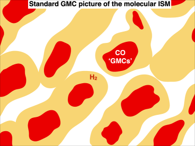
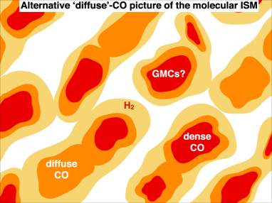
Figure 4: Top: ISM where CO solely traces star-forming GMCs. Bottom: CO (orange and red) is more pervasive than star forming clouds (red) in the molecular ISM.

Figure 4 shows a diagram of the hierarchical ISM, differentiating the scenario where CO only traces GMCs, and that where CO exists more pervasively. In the standard framework, CO only traces GMCs, which are the exclusive sites of star formation. A sub-linear KS relationship modifies this description to include CO in more diffuse regions, as depicted in the bottom panel of Figure 4. Future observational analyses are needed to quantify the relative amounts of dense and diffuse molecular gas, as well as the physical properties of these phases.

6 Further implications of diffuse CO emission

Both our work here, along with that of Wilson & Walker (1994), Rosolowsky et al. (2007), and Pety et al. (2013) suggest that a large fraction of the CO ($J=1-0$) intensity should be attributed to the diffuse molecular component, consisting of at least 30% of the total molecular mass from extragalactic observations. The kinematic distance ambiguity presents an additional important challenge in Galactic observations, though the contribution from diffuse molecular gas may be constrained statistically. Having ¹³CO observations may help in distinguishing the diffuse and dense phases. As the CO ($J=1-0$) line is optically thick, it may be impossible to unambiguously identify the star-forming clouds from the intercloud medium.

Another possibility for distinguishing between the phases is through higher level CO transitions. These lines require higher temperatures and/or densities for excitation. Krumholz & Thompson (2007) and Narayanan et al. (2008) suggest that the inferred KS index of higher level CO transitions should be less than the derived $N_{\rm mol}$ from the ($J=1-0$) line. In their proposition, the ($J=1-0$) should recover the underlying star formation law. This occurs because this line is thermalized almost everywhere, due to its low critical density, and thus faithfully follows the intrinsic star formation law. However, the upper level transitions have higher critical densities, and thus only trace a small fraction of the molecular content. They suggest that this leads to a shallower inferred KS slope. It will be interesting to compare the inferred relationships using different tracers, which should be possible with ALMA (as well as the JCMT NGLS survey, Wilson et al., 2009).

Finally, we note that since CO cannot be used as a reliable cloud tracer, the parameters of the integrated spectral line might neither provide accurate information about cloud dynamics, nor about the $X_{\rm CO}$ factor. Nevertheless, cloud properties such as mass, velocity dispersion, and virial state are often estimated from the CO ($J=1-0$) line. Results from these analyses are certainly affected by the assumption that CO neatly traces clouds, as well as the uncertainties raised above (see also Pringle et al., 2001). As elucidated by Maloney (1990), the standard $X_{\rm CO}$ factor can be derived analytically based on the assumption of virial equilibrium, since both the mass and luminosity are set by the CO linewidth (see also Shetty et al., 2011b; Wall, 2007; Narayanan & Hopkins, 2013). Consequently, the presence of diffuse emission complicates any investigation of cloud structure and dynamics solely from CO observations.

7 Summary

We have examined possible physical interpretations of the sublinear KS relationship (SKB13 Blanc et al., 2009; Ford et al., 2013; Shetty et al., 2014). In Section 3.1, we indicated that if CO uniquely traces star-forming clouds, then cloud properties such as the volume density or star formation efficiency must differ between clouds. Similarly, we discussed variations in the $X_{\rm CO}$ factor in Section 3.2.

The third possibility, considered in Section 3.3, is the presence of substantial amounts of diffuse molecular gas which also contributes towards the total CO luminosity. As the star formation rate is expected to be linearly correlated with dense gas, then the resulting KS index $N_{\rm mol}$ depends on $f_{\rm diff}$. Galaxies with $N_{\rm mol}$ $<$ 1, such as M51, have $f_{\rm diff}$ (dense gas fractions $f_{\rm den}$) increasing (decreasing) with $\Sigma_{\rm mol}$. Accordingly, we expect $f_{\rm diff}$ to drop at larger radii where $\Sigma_{\rm mol}$ decreases. Since the KS relationships are different between galaxies, the $f_{\rm diff}$$-$ $\Sigma_{\rm mol}$ correlations also correspondingly vary. Indeed, observations including higher level CO transitions as well as ¹³CO indicate the presence of substantial amounts of CO in a diffuse component consisting of  $\buildrel>\over{\sim}$  30%. This phase may exist in the form of low mass  ($\buildrel<\over{\sim}$ 10⁴ M_⊙) clouds, or as a hierarchical and pervasive medium.

Quantifying the amounts of gas in the various phases is necessary for understanding the timescales associated with star formation. We suggest that the sublinearity in the KS relationship is directly due to the dominant contribution of diffuse CO gas, with large $f_{\rm diff}$. This results in a long CO depletion time, which in the case of M51, varies from $\sim$1.7 to  $\buildrel<\over{\sim}$ 3 Gyr for 25  $\buildrel<\over{\sim}$  $\Sigma_{\rm mol}$  $\buildrel<\over{\sim}$  200 M_⊙ pc^-2. If collapse only occurs in dense gas at a constant timescale, then for galaxies such as M51 with $N_{\rm mol}$ $\approx$ 0.7 the fraction of CO traced gas currently forming stars is only of order 0.1% or less. Future observational analysis, including other ISM tracers, should further reveal the role of the different phases, including the timescales and efficiencies in the phase transitions towards the formation of stars.

References

- Ballesteros-Paredes & Mac Low (2002) Ballesteros-Paredes J., Mac Low M.-M., 2002, ApJ, 570, 734
- Battisti & Heyer (2014) Battisti A. J., Heyer M. H., 2014, ApJ, 780, 173
- Beaumont et al. (2013) Beaumont C. N., Offner S. S. R., Shetty R., Glover S. C. O., Goodman A. A., 2013, ApJ, 777, 173
- Bigiel et al. (2010) Bigiel F., Leroy A., Walter F., Blitz L., Brinks E., de Blok W. J. G., Madore B., 2010, AJ, 140, 1194
- Bigiel et al. (2008) Bigiel F., Leroy A., Walter F., Brinks E., de Blok W. J. G., Madore B., Thornley M. D., 2008, AJ, 136, 2846
- Blanc et al. (2009) Blanc G. A., Heiderman A., Gebhardt K., Evans, II N. J., Adams J., 2009, ApJ, 704, 842
- Blitz et al. (1984) Blitz L., Magnani L., Mundy L., 1984, ApJL, 282, L9
- Bolatto et al. (2013) Bolatto A. D., Wolfire M., Leroy A. K., 2013, ARA&A, 51, 207
- Burgh et al. (2007) Burgh E. B., France K., McCandliss S. R., 2007, ApJ, 658, 446
- Caldú-Primo et al. (2013) Caldú-Primo A., Schruba A., Walter F., Leroy A., Sandstrom K., de Blok W. J. G., Ianjamasimanana R., Mogotsi K. M., 2013, AJ, 146, 150
- Dickman et al. (1986) Dickman R. L., Snell R. L., Schloerb F. P., 1986, ApJ, 309, 326
- Dobbs et al. (2011) Dobbs C. L., Burkert A., Pringle J. E., 2011, MNRAS, 417, 1318
- Dobbs et al. (2013) Dobbs C. L. et al., 2013, ArXiv e-prints
- Elmegreen (1993a) Elmegreen B. G., 1993a, in Protostars and Planets III, Levy E. H., Lunine J. I., eds., pp. 97–124
- Elmegreen (1993b) Elmegreen B. G., 1993b, ApJL, 419, L29
- Elmegreen (1993c) Elmegreen B. G., 1993c, ApJ, 411, 170
- Elmegreen (1994) Elmegreen B. G., 1994, ApJL, 425, L73
- Elmegreen (2002) Elmegreen B. G., 2002, ApJ, 577, 206
- Elmegreen (2013) Elmegreen B. G., 2013, in IAU Symposium, Vol. 292, IAU Symposium, Wong T., Ott J., eds., pp. 35–38
- Elmegreen & Scalo (2004) Elmegreen B. G., Scalo J., 2004, ARA&A, 42, 211
- Falgarone et al. (1992) Falgarone E., Puget J.-L., Perault M., 1992, A&A, 257, 715
- Ford et al. (2013) Ford G. P. et al., 2013, ApJ, 769, 55
- Gammie et al. (2003) Gammie C. F., Lin Y.-T., Stone J. M., Ostriker E. C., 2003, ApJ, 592, 203
- Gao & Solomon (2004) Gao Y., Solomon P. M., 2004, ApJ, 606, 271
- Gelman et al. (2004) Gelman A., Carlin J. B., Stern H. S., Rubin D. B., 2004, Bayesian Data Analysis: Second Edition. Chapman & Hall
- Gelman & Hill (2007) Gelman A., Hill J., 2007, Data Analysis Using Regression and Multilevel/Hierarchical Modeling. Cambridge University Press
- Gil de Paz et al. (2007) Gil de Paz A. et al., 2007, ApJS, 173, 185
- Glover & Clark (2012) Glover S. C. O., Clark P. C., 2012, MNRAS, 421, 9
- Glover & Mac Low (2011) Glover S. C. O., Mac Low M., 2011, MNRAS, 412, 337
- Heiderman et al. (2010) Heiderman A., Evans, II N. J., Allen L. E., Huard T., Heyer M., 2010, ApJ, 723, 1019
- Helfer et al. (2003) Helfer T. T., Thornley M. D., Regan M. W., Wong T., Sheth K., Vogel S. N., Blitz L., Bock D. C.-J., 2003, ApJS, 145, 259
- Hopkins et al. (2011) Hopkins P. F., Quataert E., Murray N., 2011, MNRAS, 417, 950
- Hughes et al. (2013) Hughes A. et al., 2013, ApJ, 779, 44
- Kelly (2007) Kelly B. C., 2007, ApJ, 665, 1489
- Kennicutt & Evans (2012) Kennicutt R. C., Evans N. J., 2012, ARA&A, 50, 531
- Kennicutt (1989) Kennicutt, Jr. R. C., 1989, ApJ, 344, 685
- Kennicutt (1998) Kennicutt, Jr. R. C., 1998, ApJ, 498, 541
- Kennicutt et al. (2003) Kennicutt, Jr. R. C. et al., 2003, PASP, 115, 928
- Kim et al. (2011) Kim C.-G., Kim W.-T., Ostriker E. C., 2011, ApJ, 743, 25
- Kim et al. (2013) Kim J.-h., Krumholz M. R., Wise J. H., Turk M. J., Goldbaum N. J., Abel T., 2013, ApJ, 779, 8
- Kruijssen & Longmore (2014) Kruijssen J. M. D., Longmore S. N., 2014, ArXiv e-prints
- Krumholz (2012) Krumholz M. R., 2012, ApJ, 759, 9
- Krumholz et al. (2011) Krumholz M. R., Leroy A. K., McKee C. F., 2011, ApJ, 731, 25
- Krumholz & McKee (2005) Krumholz M. R., McKee C. F., 2005, ApJ, 630, 250
- Krumholz & Thompson (2007) Krumholz M. R., Thompson T. A., 2007, ApJ, 669, 289
- Kruschke (2011) Kruschke J. K., 2011, Doing Bayesian Data Analysis. Elsevier Inc.
- Lada et al. (2012) Lada C. J., Forbrich J., Lombardi M., Alves J. F., 2012, ApJ, 745, 190
- Lada et al. (2010) Lada C. J., Lombardi M., Alves J. F., 2010, ApJ, 724, 687
- Lee et al. (2014) Lee M.-Y., Stanimirovic S., Wolfire M. G., Shetty R., Glover S. C. O., Molina F. Z., Klessen R. S., 2014, ArXiv e-prints
- Leroy et al. (2011) Leroy A. K. et al., 2011, ApJ, 737, 12
- Leroy et al. (2009) Leroy A. K. et al., 2009, AJ, 137, 4670
- Leroy et al. (2008) Leroy A. K., Walter F., Brinks E., Bigiel F., de Blok W. J. G., Madore B., Thornley M. D., 2008, AJ, 136, 2782
- Leroy et al. (2013) Leroy A. K. et al., 2013, AJ, 146, 19
- Liszt et al. (2010) Liszt H. S., Pety J., Lucas R., 2010, A&A, 518, A45+
- Liu et al. (2011) Liu G., Koda J., Calzetti D., Fukuhara M., Momose R., 2011, ApJ, 735, 63
- Mac Low & Klessen (2004) Mac Low M., Klessen R. S., 2004, Reviews of Modern Physics, 76, 125
- Magnani et al. (2000) Magnani L., Hartmann D., Holcomb S. L., Smith L. E., Thaddeus P., 2000, ApJ, 535, 167
- Maloney (1990) Maloney P., 1990, ApJL, 348, L9
- Maloney & Black (1988) Maloney P., Black J. H., 1988, ApJ, 325, 389
- McKee & Ostriker (2007) McKee C. F., Ostriker E. C., 2007, ARA&A, 45, 565
- Momose et al. (2013) Momose R. et al., 2013, ApJL, 772, L13
- Murray (2011) Murray N., 2011, ApJ, 729, 133
- Murray & Rahman (2010) Murray N., Rahman M., 2010, ApJ, 709, 424
- Narayanan et al. (2008) Narayanan D., Cox T. J., Shirley Y., Davé R., Hernquist L., Walker C. K., 2008, ApJ, 684, 996
- Narayanan & Hopkins (2013) Narayanan D., Hopkins P. F., 2013, MNRAS, 433, 1223
- Narayanan et al. (2011) Narayanan D., Krumholz M., Ostriker E. C., Hernquist L., 2011, MNRAS, 418, 664
- Narayanan et al. (2012) Narayanan D., Krumholz M. R., Ostriker E. C., Hernquist L., 2012, MNRAS, 421, 3127
- Onishi et al. (2001) Onishi T., Yoshikawa N., Yamamoto H., Kawamura A., Mizuno A., Fukui Y., 2001, PASJ, 53, 1017
- Onodera et al. (2010) Onodera S. et al., 2010, ApJL, 722, L127
- Ostriker et al. (2010) Ostriker E. C., McKee C. F., Leroy A. K., 2010, ApJ, 721, 975
- Ostriker & Shetty (2011) Ostriker E. C., Shetty R., 2011, ApJ, 731, 41
- Pety et al. (2013) Pety J. et al., 2013, ApJ, 779, 43
- Polk et al. (1988) Polk K. S., Knapp G. R., Stark A. A., Wilson R. W., 1988, ApJ, 332, 432
- Pringle et al. (2001) Pringle J. E., Allen R. J., Lubow S. H., 2001, MNRAS, 327, 663
- Rahman et al. (2011) Rahman N. et al., 2011, ApJ, 730, 72
- Rahman et al. (2012) Rahman N. et al., 2012, ApJ, 745, 183
- Rosolowsky et al. (2007) Rosolowsky E., Keto E., Matsushita S., Willner S. P., 2007, ApJ, 661, 830
- Rubio et al. (2004) Rubio M., Boulanger F., Rantakyro F., Contursi A., 2004, A&A, 425, L1
- Sandstrom et al. (2013) Sandstrom K. M. et al., 2013, ApJ, 777, 5
- Scalo (1990) Scalo J., 1990, in Astrophysics and Space Science Library, Vol. 162, Physical Processes in Fragmentation and Star Formation, Capuzzo-Dolcetta R., Chiosi C., di Fazio A., eds., pp. 151–176
- Scalo & Elmegreen (2004) Scalo J., Elmegreen B. G., 2004, ARA&A, 42, 275
- Schinnerer et al. (2013) Schinnerer E. et al., 2013, ApJ, 779, 42
- Schmidt (1959) Schmidt M., 1959, ApJ, 129, 243
- Schruba et al. (2011) Schruba A. et al., 2011, AJ, 142, 37
- Schruba et al. (2010) Schruba A., Leroy A. K., Walter F., Sandstrom K., Rosolowsky E., 2010, ApJ, 722, 1699
- Shetty et al. (2010) Shetty R., Collins D. C., Kauffmann J., Goodman A. A., Rosolowsky E. W., Norman M. L., 2010, ApJ, 712, 1049
- Shetty et al. (2011a) Shetty R., Glover S. C., Dullemond C. P., Klessen R. S., 2011a, MNRAS, 412, 1686
- Shetty et al. (2011b) Shetty R., Glover S. C., Dullemond C. P., Ostriker E. C., Harris A. I., Klessen R. S., 2011b, MNRAS, 415, 3253
- Shetty et al. (2013) Shetty R., Kelly B. C., Bigiel F., 2013, MNRAS, 430, 288
- Shetty et al. (2014) Shetty R., Kelly B. C., Rahman N., Bigiel F., Bolatto A. D., Clark P. C., Klessen R. S., Konstandin L. K., 2014, MNRAS, 437, L61
- Shetty & Ostriker (2008) Shetty R., Ostriker E. C., 2008, ApJ, 684, 978
- Solomon & Rivolo (1989) Solomon P. M., Rivolo A. R., 1989, ApJ, 339, 919
- Solomon et al. (1987) Solomon P. M., Rivolo A. R., Barrett J., Yahil A., 1987, ApJ, 319, 730
- van Dishoeck & Black (1988) van Dishoeck E. F., Black J. H., 1988, ApJ, 334, 771
- Wall (2007) Wall W. F., 2007, MNRAS, 379, 674
- Wilson & Walker (1994) Wilson C. D., Walker C. E., 1994, ApJ, 432, 148
- Wilson et al. (2012) Wilson C. D. et al., 2012, MNRAS, 424, 3050
- Wilson et al. (2009) Wilson C. D. et al., 2009, ApJ, 693, 1736
- Wu et al. (2005) Wu J., Evans, II N. J., Gao Y., Solomon P. M., Shirley Y. L., Vanden Bout P. A., 2005, ApJL, 635, L173