Active Brownian particles: Entropy production and fluctuation-response

Abstract

Within the Rayleigh-Helmholtz model of active Brownian particles activity is due to a non-linear velocity dependent force. In the presence of external trapping potential or constant force, the steady state of the system breaks detailed balance producing a net entropy. Using molecular dynamics simulations, we obtain the probability distributions of entropy production in these steady states. The distribution functions obey fluctuation theorems for entropy production. Using the simulation, we further show that the steady state response function obeys a modified fluctuation-dissipation relation.

I Introduction

Active systems perform out of equilibrium dynamics by generating motion utilizing energy from their environment. This is unlike non-equilibrium state of passive particles, where the system is driven by external forces. Examples of active system range from moving animals, to motile cells, motor proteins, and artificial active Brownian particles (ABP) Romanczuk2012 ; Vicsek2012 , e.g., self-propelled colloids Howse2007 ; Zheng2013 , nano-rotors Nourhani2013 , vibrated granular particles Feitosa2004 ; Joubaud2012 . Generation of self-propulsion is often expressible in terms of non-linear velocity dependent forces that lead to non-zero mean speed at steady state Romanczuk2012 .

Properties of small systems, in or out of equilibrium, are describable within the framework of stochastic thermodynamics Sekimoto1998 ; Bustamante2005 ; Seifert2012 . Probability distributions of work done, or entropy production are shown to obey fluctuation theorems in driven passive systems, e.g., of small assembly of nano-particles, colloids, granular matter, and polymers Jarzynski2011 ; Jarzynski1997 ; Crooks1999 ; Wang2002 ; Liphardt2002 ; Feitosa2004 ; Narayan2004 ; Kurchan2007 . While the mean entropy production in such processes remain positive, occasional fluctuation of negative entropy production is not ruled out Evans1993 ; Gallavotti1995 ; Lebowitz1999 . The stochastic entropy production by particles is associated with their trajectories Seifert2005 ; Seifert2008 . Fluctuation theorems have been verified in experiments on colloids Wang2002 ; Blickle2006 ; Speck2007 , granular matter Joubaud2012 , and used to find out the free energy landscape of RNA Liphardt2002 ; Collin2005 . Fluctuation theorems have also been derived for models of molecular motors Seifert2011 ; Lacoste2011 ; Lacoste2009 , and used to determine autonomous force or torque generation by them Hayashi2010 ; Hayashi2012 . Recently, fluctuation theorems for entropy production have been extended for ABPs with velocity dependent self-propulsion forces Ganguly2013 . On the other hand, the non-equilibrium steady states (NESS) of driven passive Brownian particles are characterized by response functions that obey modified fluctuation-dissipation relations (MFDR) in terms of steady state correlations Cugliandolo1994 ; Speck2006 ; Baiesi2009 ; Prost2009 ; Seifert2010 ; Verley2011 ; Chaudhuri2012 . Theoretical predictions in this context were verified experimentally Blickle2007 ; Gomez-Solano2009 .

In this paper, we consider the Rayleigh-Helmholtz model Romanczuk2012 of active Brownian particles (ABP) where activity is generated via a non-linear velocity dependent force. Starting from underdamped Langevin equations, we derive fluctuation theorems for entropy production by ABPs. We perform molecular dynamics simulations in the presence of Langevin thermostat to obtain probability distributions of entropy production to find good agreement with the detailed fluctuation theorem. Finally we characterize non-equilibrium steady states of ABPs in terms of a modified fluctuation-dissipation relation.

II Model

The dynamics of an ABP in the presence of a velocity dependent active force $F(v)$ can be described in terms of the Langevin equations of motion

$$\dot{x} = v$$

$$\dot{v} = -\gamma v+\eta(t)+F(v)-\partial_{x}U(x)+f(t).$$ (1)

The Langevin heat bath is characterized by the viscous dissipation $-\gamma v$ and Gaussian white noise $\eta(t)$ obeying $\langle\eta(t)\rangle=0$, $\langle\eta(t)\eta(t^{\prime})\rangle=2D_{0}\delta(t-t^{\prime})$ with $D_{0}=\gamma k_{B}T$. Here $T$ denotes an effective temperature representing both thermal, and non-thermal fluctuations that may arise from chemical processes leading to activity. In the above equation $U(x)$ denotes a conservative potential, and $f(t)$ a time-dependent control force. We use particle mass $m=1$ throughout this paper.

The generation of activity by $F(v)$ can be seen easily considering $U(x)=0=f(t)$. In the over-damped limit, the mean velocity is obtainable from the relation $\gamma\langle v\rangle-F(\langle v\rangle)=0$. Within the Rayleigh-Helmholtz model $F(v)=av-bv^{3}$ with $a>\gamma$. This leads to three possible fixed-points for the steady state mean velocity $\langle v\rangle=0,\pm v_{0}$ with $v_{0}=\sqrt{(a-\gamma)/b}$, among which $\langle v\rangle=0$ is unstable and $\pm v_{0}$ are stable fixed points. At small velocities, $v<v_{0}$, velocity dependent force $g(v)=F(v)-\gamma v=b(v_{0}^{2}-v^{2})v$ pumps energy into the kinetic degrees of freedom to generate self propulsion Romanczuk2012 . This model of ABPs has been successfully used to analyze the bidirectional motion of microtubule interacting with NK11 motor-proteins that generate active drive hydrolyzing the chemical fuel ATP Badoual2002 ; Endow2000 .

The Fokker-Planck equation corresponding to Eq.(1) is given by

$$\partial_{t}P(x,v,t) = -\partial_{x}(vP)-\partial_{v}[g(v)+\bar{\cal F}]P$$ (3)

$$+D_{0}\partial_{v}^{2}P\equiv-\nabla.{\bf j}$$

where $\nabla=(\partial_{x},\partial_{v})$ and $\bar{\cal F}=f(t)-\partial_{x}U$. For a time-independent external force $f$, one may express the total current ${\bf j}={\bf j}_{r}+{\bf j}_{d}$ with ${\bf j}_{r}=(vP,\bar{\cal F}P)$ the time-reversible part of the phase-space probability current, ${\bf j}_{d}=(0,g(v)P-D_{0}\partial_{v}P)$ the dissipative part of the current. The detailed balance condition, obeying microscopic time-reversal symmetry, is satisfied if ${\bf j}_{d}=(0,0)$ and $\nabla.{\bf j}_{r}=0$ Risken1989 ; Sarracino2013 . The breakdown of time-reversal symmetry leads to entropy production. Thus we consider the detailed balance condition, and its break down in the following.

II.1 Equilibrium detailed balance

The condition ${\bf j}_{d}=(0,0)$ implies

$$\partial_{v}P(x,v)=\frac{g(v)}{D_{0}}P(x,v)$$ (4)

which has a solution

$$P(x,v)=p(x)\exp[-\phi(v)/D_{0}]$$ (5)

where $\phi(v)$ is a velocity dependent potential such that $g(v)=-\partial_{v}\phi(v)$. The other condition $\nabla.{\bf j}_{r}=0$ can be written as,

$$v\partial_{x}P(x,v)+\bar{\cal F}\partial_{v}P(x,v)=0$$ (6)

in which using $P(x,v)=p(x)\exp[-\phi(v)/D_{0}]$ one obtains a solution

$$p(x)=p_{0}\exp\left[-\frac{g(v)}{vD_{0}}\,\int\bar{\cal F}dx\right].$$ (7)

If the force $\bar{\cal F}$ is conservative, $\bar{\cal F}=-\partial_{x}U$, the solution has a normalizable form $p(x)=p_{0}\exp(U(x)\,g(v)/vD_{0})$. For passive particles $g(v)=-\gamma v$ leads to Boltzmann distribution $p(x)=p_{0}\exp(-U(x)/k_{B}T)$.

On the other hand if $\bar{\cal F}$ contains a non-conservative force $f$ the solution $p(x)$ is proportional to $\exp(-fx\,g(v)/vD_{0})$, which is not normalizable as $\int_{-\infty}^{\infty}dx\exp(-fx\,g(v)/vD_{0})$ is not bounded above. Thus non-conservative force does not support a detailed balance steady state. The requirement that conservative force, not the non-conservative one, supports microscopic reversibility is shown in Ref. Tome2010 , considering a many particle system.

As we show now, even conservative force, $\bar{\cal F}=-\partial_{x}U$, does not allow detailed balance in ABPs. Using the solution given by Eq.s (5) and (7) in Eq.(4) one gets a condition

$$g(v)=-\partial_{v}\phi(v)+\partial_{v}\left(\frac{g(v)}{v}\right)U(x).$$ (8)

Since, $g(v)=-\partial_{v}\phi(v)$, the above condition is satisfied only if $g(v)\propto v$, or $U(x)=0$. For passive Brownian particles, $g(v)=-\gamma v$ and conservative force always leads to equilibrium detailed balance. Due to non-linear velocity dependence in $g(v)$, for ABPs in potential trap Eq.(8) is not satisfied, and thus detailed balance is not obeyed.

To summarize the discussion in this section, microscopic reversibility for ABPs may be broken either by imposing non-conservative external force $f$, or by trapping the ABPs in conservative external potential $U(x)$. Both these conditions, therefore, would lead to entropy production in ABPs, and are considered in this paper.

Within the Rayleigh-Helmholtz model $g(v)=(a-\gamma)v-bv^{3}$, and detailed balance is obtained if both $f=0$ and $U=0$, i.e., $\bar{\cal F}=0$. Eq.(6) implies $\partial_{x}P(x,v)=0$, which is automatically satisfied by the solution (5) with $p(x)=$ constant. Thus one gets a equilibrium-like solution for the Rayleigh-Helmholtz model

$$P_{s}(v)={\cal N}\exp[-\phi(v)/D_{0}]$$ (9)

where ${\cal N}$ is the normalization constant, and $\phi(v)=\psi(v)+\gamma v^{2}/2$ with $\psi(v)=-(a/2)v^{2}+(b/4)v^{4}$ a velocity-dependent double- well potential characterizing the self propulsion force $F(v)=-\partial_{v}\psi(v)$ of the Rayleigh-Helmholtz model. The minima of the potential $\phi(v)$ are at $\pm v_{0}$.

II.2 Non-equilibrium steady states

The non-equilibrium steady state in the presence of a constant external force $f$, and absence of potential $U=0$, may be solved easily by noting that the force may be incorporated by redefining the velocity-dependent potential to $\phi(v)-fv$. The corresponding steady state distribution is

$$P_{s}(v)={\cal N}\exp[-\{\phi(v)-fv\}/D_{0}].$$ (10)

A part of the total entropy change between two steady states is the difference in stochastic system entropy $s=-k_{B}\ln P_{s}$ Crooks1999 ; Seifert2005 , as will be discussed in the next section, and thus calculation of steady state distributions is important in the context of transient fluctuation theorems.

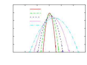
Figure 1: (Color online) Steady state probability distribution $P_{s}(v)$ for ABPs under a constant external force $f=0.2$. Points are from MD simulations, and the line is a plot of Eq.(10).

The Rayleigh-Helmholtz ABPs may also be brought into non-equilibrium steady state by trapping them within a conservative potential $U(x)$. The analytic form of the corresponding steady state solution for general $U(x)$ is not known. Thus we use numerical simulations to calculate these distributions.

We perform molecular dynamics (MD) simulations using the standard velocity-Verlet algorithm with a time-step $\delta t=0.01\tau$, where $\tau=1/\gamma$, and keep the temperature constant at $T=1.0(D_{0}/\gamma k_{B})$ via a Langevin thermostat. The simulation method for ABPs is validated by calculating the steady state velocity distribution under constant external force and comparing it against Eq.(10) (see Fig 1). In all our simulations we used $F(v)=av-bv^{3}$ with $a=4$ and $b=1$. Also, unless otherwise specified, we used the noise strength $D_{0}=1$.

III Entropy production

The Langevin equation of the Rayleigh-Helmholtz model of ABPs, obeys energy conservation. Multiplying Eq.(1) by velocity $v$ and integrating over a small time interval ${\tau_{0}}$ one obtains Sekimoto1998

$$\Delta E=\Delta W+\Delta q,$$ (11)

where $\Delta E$ denotes the change in mechanical energy $E=(1/2)v^{2}+U(x)$, $\Delta W=\int^{\tau_{0}}dt\,v.f(t)$ the work done on the ABPs by external force $f(t)$, and $\Delta q=\Delta Q+\Delta Q_{m}$ the total energy absorbed by the mechanical degrees of freedom of the ABPs: (a) from the Langevin heat bath $\Delta Q=\int^{\tau_{0}}dt\,v.(-\gamma v+\eta)$, and (b) from the self-propulsion mechanism $\Delta Q_{m}=\int^{\tau_{0}}dt\,v.F(v)$.

In a system of conventional passive Brownian particles, the stochastic entropy production in any process has two components. One is the entropy change in the system $\Delta s$ where the stochastic system-entropy is expressed as $s=-k_{B}\ln P_{s}$ with $P_{s}$ denoting steady state distribution. The other contribution comes from the change in entropy in the heat-bath, $\Delta s_{r}=-\Delta q/T$ Seifert2005 . A direct extension of this idea to ABPs would mean $\Delta s_{r}=-\Delta q/T$ with $\Delta q=\Delta Q+\Delta Q_{m}$. However, as we show below, $\Delta s_{r}$ for ABPs has further extra contributions coming from the mechanism of active force generation and its coupling to the mechanical forces Ganguly2013 .

Consider the time evolution of an ABP from $t=0$ to $\tau_{0}$ through a path defined by $X=\{x(t),v(t),f(t)\}$. The motion on this trajectory involves interaction of the particle with Langevin heat bath, and the presence of self propulsion force $F(v)$. Microscopic reversibility means the probability of such a trajectory is the same as the probability of the corresponding time-reversed trajectory. Entropy production requires break down of such microscopic reversibility.

Let us first consider the transition probability $p_{i}^{+}(x^{\prime},v^{\prime},t+\delta t|x,v,t)$ for an infinitesimal section of the trajectory evolved during a time interval $\delta t$, assuming that the whole trajectory is made up of $i=1,\dots,N$ such segments such that $N\delta t={\tau_{0}}$. The Gaussian random noise at $i$-th instant is described by $P(\eta_{i})=(\delta t/4\pi D_{0})^{1/2}\exp(-\delta t\,\eta_{i}^{2}/4D_{0})$. The transition probability is given by $p_{i}^{+}=J_{\eta_{i},v_{i}}\langle\delta(\dot{x}_{i}-v_{i})\delta(\dot{v}_{i}-{\cal F}_{i})\rangle=J_{\eta_{i},v_{i}}\int d\eta_{i}P(\eta_{i})\delta(\dot{x}_{i}-v_{i})\delta(\dot{v}_{i}-{\cal F}_{i})$, where the total force acting on the particle at $i$-th instant of time is ${\cal F}_{i}=\eta_{i}+g(v_{i})-\partial_{x_{i}}U(x_{i})+f_{i}$, with $g(v_{i})=F(v_{i})-\gamma v_{i}$, and $J_{\eta_{i},v_{i}}=(1/\delta t)[1-\delta t\,\partial_{v_{i}}g(v_{i})/2]$ (see Appendix-A). Thus we have $p_{i}^{+}=J_{\eta_{i},v_{i}}(\delta t/4\pi D_{0})^{1/2}\delta(\dot{x}_{i}-v_{i})\exp[-\frac{\delta t}{4D_{0}}\{\dot{v}_{i}-g(v_{i})+\partial_{x_{i}}U(x_{i})-f_{i}\}^{2}]$. The probability of full trajectory is ${\cal P}_{+}=\prod_{i=1}^{N}p_{i}^{+}$.

Reversing the velocities gives us the time reversed path $X^{\dagger}=\{x^{\prime}(t^{\prime}),v^{\prime}(t^{\prime}),f^{\prime}(t^{\prime})\}=\{x({\tau_{0}}-t),-v({\tau_{0}}-t),f({\tau_{0}}-t)\}$, the probability of which can be expressed as ${\cal P}_{-}=\prod_{i=1}^{N}p_{i}^{-}$ where $p_{i}^{-}=J_{\eta_{i},v_{i}}(\delta t/4\pi D_{0})^{1/2}\delta(\dot{x}_{i}-v_{i})\exp[-\frac{\delta t}{4D_{0}}\{\dot{v}_{i}+g(v_{i})+\partial_{x_{i}}U(x_{i})-f_{i}\}^{2}]$, since the velocity dependent forces are odd function of velocity $g(-v_{i})=-g(v_{i})$, and $J_{\eta_{i},v_{i}}$ remains the same.

The ratio of probabilities of the forward and reverse trajectories is

$$\frac{{\cal P}_{+}}{{\cal P}_{-}} = \exp\left[{\frac{\delta t}{D_{0}}\sum_{i=1}^{N}\left(\dot{v}_{i}+\partial_{x_{i}}U-f_{i}\right)}g(v_{i})\right]$$

$$= \exp\left[{\frac{1}{D_{0}}\int_{0}^{\tau_{0}}dt\left(\dot{v}+\frac{\partial U}{\partial x}-f(t)\right)}g(v)\right].$$

After simplifications the ratio can be expressed as Ganguly2013

$$\frac{{\cal P}_{+}}{{\cal P}_{-}} = \exp\left[-\beta\left(\Delta q+\Delta Q_{em}+\frac{1}{\gamma}\Delta\psi\right)\right]$$ (12)

where $\beta=1/k_{B}T=\gamma/D_{0}$. In the above relation $\Delta q=\Delta Q+\Delta Q_{m}$ is the heat absorbed, as identified in the context of energy conservation. The term $\Delta Q_{em}=(1/\gamma)\int_{0}^{\tau_{0}}dt\,F(v).(f(t)-\partial_{x}U)$ is a coupling between the self-propulsion and external forces. $\Delta\psi$ is the change in a self-propulsion potential defined through $F(v)=-\partial_{v}\psi(v)$.

Figure 2: (Color online) Probability distribution of total entropy production $\rho(\Delta s_{t})$ calculated in the presence of an external force $f=0.2$. The calculations are performed after collecting data over $\tau_{0}=2.56,5.12,10.24,20.48,40.96\,\tau$.

The probability ratio of the forward and reverse trajectories accounts for the entropy change in the reservoirs ${\cal P}_{+}/{\cal P}_{-}=\exp(\Delta s_{r}/k_{B})$ Seifert2005 ; Ganguly2013 . Thus we have

$$\Delta s_{r}=-\frac{1}{T}\left(\Delta q+\Delta Q_{em}+\frac{1}{\gamma}\Delta\psi\right).$$ (13)

Evidently the reservoir entropy change $\Delta s_{r}$ has contributions from two extra terms, $\Delta Q_{em}$ and $\Delta\psi$, with respect to the expression $\Delta s_{r}=-\Delta q/T$, inferred from the behavior of passive Brownian particles.

It is interesting to note that the active force has three contributions to entropy production. Origin of $\Delta Q_{m}$ in $\Delta q=\Delta Q+\Delta Q_{m}$ is direct, this is due to work done by the active force. The contribution through energy transfer $\Delta Q_{em}$ is due to coupling of velocity- dependent active force to mechanical forces. Apart from that, the mechanism of active force generation through the velocity dependent potential $\psi(v)$ also contributes to entropy. The origin and meaning of these terms have easy interpretation within a simple model of active particle dynamics $\dot{v}=-\gamma(v-v_{0})+\eta(t)+f(t)$ considered in Ref.s Romanczuk2011 ; Schienbein1993 . In this model, friction $\gamma$ pumps in energy if $v<v_{0}$, and dissipates otherwise. The self propulsion force $F=\gamma v_{0}$ leads to $\Delta Q_{em}=\int dtfv_{0}$, and $\Delta\psi/\gamma=-\Delta(vv_{0})$. Thus, in this case $\Delta Q_{em}$ and $\Delta\psi/\gamma$ are equivalent to work done, and change in internal energy for driven passive Brownian particles, respectively.

Assuming the initial and final steady state distributions as $P^{i}_{s}$ and $P^{f}_{s}$ respectively, the system entropy change is $\Delta s=s_{f}-s_{i}=k_{B}\ln(P_{s}^{i}/P_{s}^{f})$. Thus the total entropy production is

$$\Delta s_{t} = \Delta s-\frac{1}{T}\left(\Delta q+\Delta Q_{em}+\frac{1}{\gamma}\Delta\psi\right)$$ (14)

$$= \Delta s-\frac{1}{T}\left(\Delta E-\Delta W+\Delta Q_{em}+\frac{1}{\gamma}\Delta\psi\right),$$

where in the last step we used the relation of energy conservation Eq.(11).

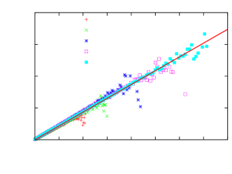
Figure 3: (Color online) Ratio of probability distributions of positive and negative entropy production $\rho(\Delta s_{t}=\Delta\sigma)/\rho(\Delta s_{t}=-\Delta\sigma)$ calculated from the data in Fig. 2. The solid line is a plot of the function $\exp(\Delta\sigma/k_{B})$.

The probability distribution of the forward process is ${\cal P}_{f}=P_{s}^{i}{\cal P}_{+}$, and that of the reverse process is ${\cal P}_{r}=P_{s}^{f}{\cal P}_{-}$. Thus

$${\cal P}_{r}/{\cal P}_{f}=\exp(-\Delta s_{t}/k_{B}),$$ (15)

and $\langle\exp(-\Delta s_{t}/k_{B})\rangle=\int{\cal D}[X]{\cal P}_{f}\exp(-\Delta s_{t}/k_{B})=\int{\cal D}[X]{\cal P}_{f}\,({\cal P}_{r}/{\cal P}_{f})=1$. This relation is known as the integral fluctuation theorem Kurchan2007 and implies a positive entropy production on an average $\langle\Delta s_{t}\rangle\geq 0$, .

Eq.(15) can be used to obtain the detailed fluctuation theorem for the probability distribution of entropy production $\rho(\Delta s_{t})$ Crooks1999 ; Ganguly2013 ,

$$\frac{\rho(\Delta\sigma)}{\rho(-\Delta\sigma)}=e^{\Delta\sigma/k_{B}},$$ (16)

where $\Delta\sigma$ denotes an amount of total entropy $\Delta s_{t}$ produced over a time interval $\tau_{0}$. In the following, using MD simulations we calculate the steady state probability distributions of total entropy productions $\rho(\Delta s_{t})$ and hence test the detailed fluctuation theorem.

III.1 Detailed balance state

In the absence of external potential $U(x)=0$, and force $f(t)=0$, the system obeys detailed balance as has been shown in Sec. II.1. Let us denote the initial and final points on a trajectory evolved over a time ${\tau_{0}}$ by $(x_{i},v_{i})$ to $(x_{f},v_{f})$. In this case, the heat absorbed $\Delta q=\Delta E=(v_{f}^{2}-v_{i}^{2})/2$, and the steady state distribution $P_{s}={\cal N}\exp[-\phi(v)/D_{0}]$ where $\phi(v)=(\gamma/2)v^{2}+\psi(v)$ with $\psi(v)=-(a/2)v^{2}+(b/4)v^{4}$. The corresponding entropy change in the system is $\Delta s/k_{B}=\Delta\phi/D_{0}=\Delta\psi/D_{0}+(\beta/2)(v_{f}^{2}-v_{i}^{2})$ with $\beta=\gamma/D_{0}$. Thus the total entropy change is

$$\frac{\Delta s_{t}}{k_{B}} = \frac{\Delta s}{k_{B}}-\beta\left(\Delta q+\frac{1}{\gamma}\Delta\psi\right)$$ (17)

$$= \frac{\Delta\phi}{D_{0}}-\frac{\beta}{2}(v_{f}^{2}-v_{i}^{2})-\frac{\Delta\psi}{D_{0}}$$

$$= 0,$$

as expected due to detailed balance. There is no difference between the initial and final steady states, and the probabilities of forward and reverse trajectories are the same.

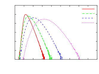
Figure 4: (Color online) Probability distributions of total entropy productions $\rho(\Delta s_{t})$ calculated in the presence of an external harmonic potential trap $U(x)=(1/2)\omega_{0}^{2}x^{2}$ with $\omega_{0}^{2}=5$. The calculations are performed after collecting data over $\tau_{0}=2.56,5.12,10.24,20.48\,\tau$.

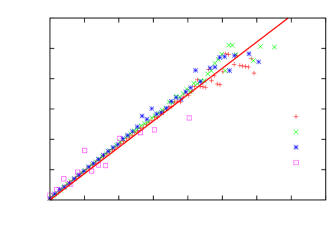
Figure 5: (Color online) Ratio of probability distributions of positive and negative entropy productions $\rho(\Delta s_{t}=\Delta\sigma)/\rho(\Delta s_{t}=-\Delta\sigma)$ calculated from the data shown in Fig. 4. The solid line shows a plot of $\exp(\Delta\sigma/k_{B})$.

III.2 NESS with constant force

The simplest non-equilibrium steady state producing entropy is attained in the presence of a constant external force, breaking the detailed balance condition for ABPs. In this case $f\neq 0$ and external potential $U(x)=0$. We assume a trajectory from $(x_{i},v_{i})$ to $(x_{f},v_{f})$ evolves over time ${\tau_{0}}$. The heat absorbed is $\Delta q=\Delta E-\Delta W=(v_{f}^{2}-v_{i}^{2})/2-f(x_{f}-x_{i})$. The steady state distribution is given by (Eq.(10)) $P_{s}={\cal N}\exp[-\{\phi(v)-fv\}/D_{0}]$ where $\phi(v)=(\gamma/2)v^{2}+\psi(v)$ with $\psi(v)=-(a/2)v^{2}+(b/4)v^{4}$. Thus the system entropy change $\Delta s/k_{B}=(\Delta\phi-f\Delta v)/D_{0}=\Delta\psi/D_{0}+(\beta/2)(v_{f}^{2}-v_{i}^{2})-(f/D_{0})(v_{f}-v_{i})$. The total entropy change is

$$\frac{\Delta s_{t}}{k_{B}} = \frac{\Delta s}{k_{B}}-\beta\left(\Delta q+\Delta Q_{em}+\frac{1}{\gamma}\Delta\psi\right)$$

$$= -\frac{f}{D_{0}}\left[(v_{f}-v_{i})+\int^{\tau_{0}}dtF(v)\right]+\beta f(x_{f}-x_{i})$$

(18)

where in the last step we used the identity $\beta\Delta Q_{em}=(f/D_{0})\int^{\tau_{0}}dtF(v)$.

In Fig. 2 we show the probability distributions of entropy production $\rho(\Delta s_{t})$ calculated from MD simulations of Rayleigh-Helmholtz ABPs at $f=0.2$, using Eq.(18) for the expression of $\Delta s_{t}$. The distributions are calculated after collecting data over various time periods ${\tau_{0}}$. Appreciable probability of negative entropy production is clearly visible. With increase in ${\tau_{0}}$, the distributions broaden and the peak positions shift towards higher values of entropy. From each curve, one can extract the ratio of probabilities $\rho(\Delta\sigma)/\rho(-\Delta\sigma)$ with $\rho(\Delta\sigma)=\rho(\Delta s_{t}=\Delta\sigma)$ and $\rho(-\Delta\sigma)=\rho(\Delta s_{t}=-\Delta\sigma)$. As is shown in Fig. 3, this ratio obeys the detailed fluctuation theorem $\rho(\Delta\sigma)/\rho(-\Delta\sigma)=\exp(\Delta\sigma/k_{B})$.

III.3 ABPs in potential trap

A system of Rayleigh-Helmholtz ABPs if trapped by an external potential $U(x)$ (keeping $f=0$) gets into a NESS. This is unlike passive Brownian particles that still remains at equilibrium with probability distribution described in terms of Boltzmann weight $\exp[-\beta U(x)]$. As we have seen in Sec. II.2, the steady state probability density $P_{s}(x,v)$ in this case is not analytically obtainable for a general $U(x)$ and noise strength $D_{0}$. We perform MD simulations to find $P_{s}(x,v)$. For a trajectory between $(x_{i},v_{i})$ and $(x_{f},v_{f})$ evolved over a time ${\tau_{0}}$, the corresponding change in the system entropy is thus calculated using the numerically obtained probability distributions, and the relation $\Delta s=k_{B}\ln[P_{s}(x_{i},v_{i})/P_{s}(x_{f},v_{f})]$. The change in the reservoir entropy is given by

$$\frac{\Delta s_{r}}{k_{B}}=-\beta\left[\Delta E-\frac{1}{\gamma}\int^{\tau_{0}}dtF(v)\partial_{x}U(x)+\frac{\Delta\psi}{\gamma}\right],$$ (19)

where $E=v^{2}/2+U(x)$, and as before, for any function $\chi(x,v)$ the change $\Delta\chi(x,v)=\chi(x_{f},v_{f})-\chi(x_{i},v_{i})$. In MD simulations, we use $U(x)=(1/2)\omega_{0}^{2}x^{2}$, a harmonic potential well with strength $\omega_{0}^{2}=5$. Probability distribution of entropy production $\rho(\Delta s_{t})$ is shown in Fig. 4. The distribution widens, and the peak rapidly moves towards very large values of total entropy as the measurement time $\tau_{0}$ is increased. The detailed fluctuation theorem is obeyed as is shown in Fig. 5.

IV Linear response at NESS: modified fluctuation dissipation relation

The steady state of the ABPs may be characterized by linear response functions. The Fokker-Planck equation (3) can be written as

$$\partial_{t}P(x,v,t)={\cal L}(x,v,h)P(x,v,t)=({\cal L}_{0}+f(t){\cal L}_{1})P$$ (20)

where

$${\cal L}_{0}P = -\partial_{x}(vP)-\partial_{v}\left[g(v)-\partial_{x}U\right]P+D_{0}\partial_{v}^{2}P$$

$${\cal L}_{1}P = -\partial_{v}P.$$

As it has been shown earlier, the linear response to $f(t)$ in a system at steady state described by $P_{s}(x,v)$ such that ${\cal L}_{0}P_{s}=0$ can be expressed as Chaudhuri2012 ; Seifert2010 ; Verley2011 ; Agarwal1972

$$\frac{\delta\langle A(t)\rangle}{\delta f(t^{\prime})}=\langle A(t)M(t^{\prime})\rangle_{s}$$ (21)

where $\langle\dots\rangle_{s}$ indicates a steady state average, and $M=-({1}/{P_{s}})\partial_{v}P_{s}$. This is a version of modified fluctuation dissipation relation (MFDR).

For free ABPs $U(x)=0=f(t)$, the system goes into a detailed balance steady state described by the distribution $P_{s}(v)={\cal N}\exp[-\phi(v)/D_{0}]$ where $\phi(v)=-(a-\gamma)v^{2}/2+bv^{4}/4$. In this case, $M=\partial_{v}[-\ln P_{s}]=g(v)/D_{0}=[-(a-\gamma)v+bv^{3})/D_{0}$, and the response function $R_{A}(t,t^{\prime})={\delta\langle A(t)\rangle}/{\delta f(t^{\prime})}$ around a steady state, where time translation invariance is obeyed, is given by

$$R_{A}(t)=-\frac{a-\gamma}{D_{0}}\langle A(t)v(0)\rangle_{s}+\frac{b}{D_{0}}\langle A(t)v^{3}(0)\rangle_{s}.$$ (22)

For the ABPs, $a>\gamma$ gives rise to active force generation leading to a negative coefficient of $\langle A(t)v(0)\rangle_{s}$ in the MFDR. Given that the fluctuation dissipation theorem for passive Brownian particles is $R_{A}(t)=\beta\langle A(t)v(0)\rangle_{eq}$, within equilibrium the temperature can be expressed as the ratio $k_{B}T=\langle A(t)v(0)\rangle_{eq}/R_{A}(t)$. For ABPs, even in a detailed balance state, the effective temperature $T$ is not expressible as a simple ratio of fluctuation $\langle A(t)v(0)\rangle_{s}$ and response $R_{A}(t)$, and the coefficient of $\langle A(t)v(0)\rangle_{s}$ can not be interpreted as an effective negative temperature.

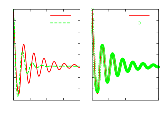
Figure 6: (Color online) Response functions and steady state fluctuations. ($a$) Direct MD evaluation of response function for Rayleigh-Helmholtz ABPs, and passive Brownian particles within a harmonic trap of strength $\omega_{0}^{2}=5$. ($b$)  Comparison of response function of ABPs $R_{v}(t)$ against steady state fluctuations as given by the right hand side of Eq.(26).

In order to use the expression Eq.(21), one requires the detailed knowledge of the steady state probability distribution. Interpreting the Gaussian noise $\eta(t)$ in the same footing as the externally applied forces, and by expressing the observable $A(x(t),v(t))$ as a functional $A[\eta(t)]$ of the noise history, the response function can also be written as Speck2006

$$R_{A}(t-t^{\prime})=\left\langle\frac{\delta A[\eta]}{\delta\eta(t^{\prime})}\right\rangle=\frac{1}{2D_{0}}\langle A(t)\eta(t^{\prime})\rangle.$$ (23)

Using the Langevin equation to replace $\eta(t^{\prime})$, for ABPs under a potential $U(x)$ one finds

$$R_{A}(t) = \frac{1}{2D_{0}}[\langle A(t)\dot{v}(0)\rangle-\langle A(t)g[v(0)]\rangle$$ (24)

$$+\langle A(t)\partial_{x}U[x(0)]\rangle].$$

Let us now focus our attention on velocity response $R_{v}(t)$ in NESS. Utilizing causality and time translation symmetry at the NESS the above expression can be written as Sarracino2013

$$R_{v}(t) = -\frac{1}{2D_{0}}[\langle g[v(t)]v(0)\rangle+\langle v(t)g[v(0)]\rangle$$ (25)

$$-\langle\partial_{x}U[x(t)]v(0)\rangle-\langle v(t)\partial_{x}U[x(0)]\rangle]$$

where $g[v(t)]=-\gamma v(t)+F[v(t)]$. For harmonic traps $U(x)=(1/2)\omega_{0}^{2}x^{2}$, the above expression further simplifies, as $\langle x(t)v(0)\rangle=-\langle v(t)x(0)\rangle$, to

$$R_{v}(t)=-\frac{1}{2D_{0}}[\,\langle g[v(t)]v(0)\rangle+\langle v(t)g[v(0)]\rangle\,].$$ (26)

Even for $U=0$ this relation holds, but the system goes to a detailed balance state, in which, due to time reversal symmetry $\langle g[v(t)]v(0)\rangle=\langle v(t)g[v(0)]\rangle$, and thus

$$R_{v}(t)=-\frac{1}{D_{0}}\langle v(t)g[v(0)]\rangle$$ (27)

which is the same as Eq.(22) for velocity response. For passive free particles, $g(v)=-\gamma v$, and one gets back the equilibrium response function $R_{v}(t)=\beta\langle v(t)v(0)\rangle=\exp(-t)$. However, when placed within a harmonic trap they are expected to show an oscillatory response.

Note that $\delta\langle v(t)\rangle=\int_{-\infty}^{t}R_{v}(t-t^{\prime})\delta f(t^{\prime})dt^{\prime}$ and replacement of the perturbing force $\delta f(t^{\prime})$ by a Diract-delta function $\delta(t^{\prime})$ gives $\delta\langle v(t)\rangle=R_{v}(t)$. Thus in MD simulations, velocity response is calculated by following the change in velocity due an impulsive force of unit magnitude. In Fig. 6($a$) we show the comparison between the response functions $R_{v}(t)$ evaluated from MD simulations of harmonically trapped passive Brownian particles with that of the Rayleigh-Helmholtz ABPs. Activity clearly leads to longer lasting oscillations. In the non-equilibrium steady state that the ABPs maintain, our simulations show $\langle g[v(t)]v(0)\rangle\neq\langle v(t)g[v(0)]\rangle$ which is due to the absence of time-reversal symmetry. We find a good agreement between the directly calculated response function $R_{v}(t)$ with that of the steady state fluctuations expressed by the right hand side of Eq.(26) (see Fig. 6($b$)). The correlation functions are calculated from a separate MD simulation performed in the absence of external force.

V conclusion

Using molecular dynamics simulations, we obtained probability distributions of entropy production in non-equilibrium steady states of the Rayleigh-Helmholtz ABPs. We identified the conditions under which ABPs break detailed balance and start to produce entropy. We showed that the entropy production obeys the detailed fluctuation theorem. Further, we verified a modified fluctuation-dissipation relation for the steady state response. Given the close relation of the Rayleigh-Helmholtz model to the bidirectional motion of microtubules influenced by NK11 motors Badoual2002 , our predictions are amenable to experimental verification.

Appendix A Probability of a trajectory

It is simpler to consider an over-damped Langevin dynamics first. Let us assume the position of a particle evolves via

$$\gamma\dot{x}=\eta(t)+{\cal F}$$ (28)

where ${\cal F}$ is the total non-stochastic force acting on the particle, and the Gaussian white noise is characterized by $\langle\eta(t)\rangle=0$, $\langle\eta(t)\eta(0)\rangle=2D_{0}\delta(t)$ with $D_{0}=\gamma k_{B}T$. Discretizing the equation with $t=i\,\delta t$, using Stratonovich rule,

$$x_{i}=x_{i-1}+\frac{\beta D}{2}({\cal F}_{i}+{\cal F}_{i-1})\delta t+\xi_{i}\delta t$$ (29)

where $D=k_{B}T/\gamma$ and $\xi_{i}=\eta_{i}/\gamma$. The Gaussian random noise $\xi(t)$ follows the distribution $P(\xi_{i})=(\delta t/4\pi D)\exp(-\delta t\xi_{i}^{2}/4D)$. Thus the transition probability $P(x_{i}|x_{i-1})=J_{\xi_{i},x_{i}}\,P(\xi)$ where the Jacobian

$$J_{\xi_{i},x_{i}}={\rm det}\left(\frac{\partial\xi_{i}}{\partial x_{i}}\right)=\frac{1}{\delta t}\left(1-\frac{\delta t}{2\gamma}\partial_{x_{i}}{\cal F}_{i}\right).$$ (30)

Using Eq.(29) to replace $\xi_{i}$, we find

$$P(x_{i}|x_{i-1})=J_{\xi_{i},x_{i}}\,\sqrt{\frac{\delta t}{4\pi D}}e^{-\frac{\delta t}{4D}\left[\frac{x^{\prime}-x}{\delta t}+\beta D{\cal F}\right]^{2}}.$$ (31)

This transition probability is easily obtainable from the probability of velocity calculated at $i$-th instant $\langle\delta(\dot{x}-v)\rangle$ where $v=(\eta+{\cal F})/\gamma$ ,

$$\langle\delta(\dot{x}-v)\rangle = \int d\xi\sqrt{\frac{\delta t}{4\pi D}}e^{-\frac{\delta t}{4D}\xi^{2}}\delta(\dot{x}-v)$$ (32)

$$= \sqrt{\frac{\delta t}{4\pi D}}e^{-\frac{\delta t}{4D}\left[\dot{x}+\beta D{\cal F}\right]^{2}}.$$

Identifying $\dot{x}=(x_{i}-x_{i-1})/\delta t$, the transition probability, or the probability of a segment of the trajectory between $(x_{i-1},t)$ and $(x_{i},t+\delta t)$ is $P(x_{i}|x_{i-1})=J_{\xi_{i},x_{i}}\,\langle\delta(\dot{x}-v)\rangle$. The whole trajectory is obtainable by adding a series of such segments. The probability weight associated with the whole trajectory is ${\cal P}^{+}=\prod_{i}P(x_{i}|x_{i-1})$ Seifert2008 .

A direct extension of this idea to under-damped Langevin equation is straightforward. The dynamics is described by

$$\dot{x} = v$$

$$\dot{v} = g(v)+\eta(t)+{\cal F}$$ (33)

where $g(v)$ contains all the velocity-dependent forces, and ${\cal F}$ denotes the velocity-independent forces. Similarly as in the above calculation, the probability of $i$-th segment of the trajectory $p^{+}_{i}\equiv P(x_{i},v_{i}|x_{i-1},v_{i-1})=J_{\eta_{i},v_{i}}\,\langle\delta(\dot{x}-v)\delta(\dot{v}-\{g(v)+{\cal F}\})\rangle$ which gives

$$p^{+}_{i}=J_{\eta_{i},v_{i}}\,\delta(\dot{x}-v)\sqrt{\frac{\delta t}{4\pi D_{0}}}e^{-\frac{\delta t}{4D_{0}}\left[\dot{v}+\gamma v-{\cal F}\right]^{2}},$$ (34)

where Ganguly2013

$$J_{\eta_{i},v_{i}}=\frac{1}{\delta t}\left(1-\frac{\delta t}{2}\partial_{v_{i}}g(v_{i})\right).$$ (35)

The probability associated with a full trajectory is ${\cal P}^{+}=\prod_{i}p^{+}_{i}$.

References

• (1) P. Romanczuk, M. Bär, W. Ebeling, B. Lindner, and L. Schimansky-Geier, The European Physical Journal Special Topics 202, 1 (2012).
• (2) T. Vicsek and A. Zafeiris, Physics Reports 517, 71 (2012).
• (3) J. R. Howse, R. A. L. Jones, A. J. Ryan, T. Gough, R. Vafabakhsh, and R. Golestanian, Physical Review Letters 99, 048102 (2007).
• (4) X. Zheng, B. ten Hagen, A. Kaiser, M. Wu, H. Cui, Z. Silber-Li, and H. Löwen, Physical Review E 88, 032304 (2013).
• (5) A. Nourhani, Y.-M. Byun, P. E. Lammert, A. Borhan, and V. H. Crespi, Physical Review E 88, 062317 (2013).
• (6) K. Feitosa and N. Menon, Physical Review Letters 92, 164301 (2004).
• (7) S. Joubaud, D. Lohse, and D. van der Meer, Physical Review Letters 108, 210604 (2012).
• (8) K. Sekimoto, Progress of Theoretical Physics Supplement 130, 17 (1998).
• (9) C. Bustamante, J. Liphardt, and F. Ritort, Physics Today 58, 43 (2005).
• (10) U. Seifert, Rep. Prog. Phys. 75, 126001 (2012).
• (11) C. Jarzynski, Annu. Rev. Condens. Matter Phys. 2, 329 (2011).
• (12) C. Jarzynski, Physical Review Letters 78, 2690 (1997).
• (13) G. E. Crooks, Physical Review E 60, 2721 (1999).
• (14) G. M. Wang, E. M. Sevick, E. Mittag, D. J. Searles, and D. J. Evans, Physical Review Letters 89, 050601 (2002).
• (15) J. Liphardt, S. Dumont, S. B. Smith, I. Tinoco, and C. Bustamante, Science (New York, N.Y.) 296, 1832 (2002).
• (16) O. Narayan and A. Dhar, J. Phys. A: Math. Gen. 37, 63 (2004).
• (17) J. Kurchan, Journal of Statistical Mechanics: Theory and Experiment 2007, P07005 (2007).
• (18) D. J. Evans, E. G. D. Cohen, and G. P. Morriss, Physical Review Letters 71, 2401 (1993).
• (19) G. Gallavotti and E. G. D. Cohen, Physical Review Letters 74, 2694 (1995).
• (20) J. Lebowitz and H. Spohn, Journal of Statistical Physics 95, 333 (1999).
• (21) U. Seifert, Physical Review Letters 95, 040602 (2005).
• (22) U. Seifert, in Soft Matter. From Synthetic to Biological Materials, LectureNotes of the 39th Spring School 2008, edited by J. K. G. Dhont, G. Gompper, G. Nägele, D. Richter, and R. G. Winkler (Forschungszentrum Jülich, Jülich, 2008), pp. 1–30.
• (23) V. Blickle, T. Speck, L. Helden, U. Seifert, and C. Bechinger, Physical Review Letters 96, 070603 (2006).
• (24) T. Speck, V. Blickle, C. Bechinger, and U. Seifert, Euro. Phys. Lett. 79, 30002 (2007).
• (25) D. Collin, F. Ritort, C. Jarzynski, S. B. Smith, I. Tinoco, and C. Bustamante, Nature 437, 231 (2005).
• (26) U. Seifert, The European physical journal. E, Soft matter 34, 1 (2011).
• (27) D. Lacoste and K. Mallick, Biological Physics 60, 61 (2011).
• (28) D. Lacoste and K. Mallick, Phys. Rev. E 80, 021923 (2009).
• (29) K. Hayashi, H. Ueno, R. Iino, and H. Noji, Physical Review Letters 104, 218103 (2010).
• (30) K. Hayashi, M. Tanigawara, and J.-i. Kishikawa, Biophysics 8, 67 (2012).
• (31) C. Ganguly and D. Chaudhuri, Physical Review E 88, 032102 (2013).
• (32) L. Cugliandolo, J. Kurchan, and G. Parisi, J. Phys. I France 4, 1641 (1994).
• (33) T. Speck and U. Seifert, Europhysics Letters (EPL) 74, 391 (2006).
• (34) M. Baiesi, C. Maes, and B. Wynants, Phys. Rev. Lett. 103, 010602 (2009).
• (35) J. Prost, J.-F. Joanny, and J. M. R. Parrondo, Physical Review Letters 103, 090601 (2009).
• (36) U. Seifert and T. Speck, EPL (Europhysics Letters) 89, 10007 (2010).
• (37) G. Verley, K. Mallick, and D. Lacoste, EPL (Europhysics Letters) 93, 10002 (2011).
• (38) D. Chaudhuri and A. Chaudhuri, Physical Review E 85, 021102 (2012).
• (39) V. Blickle, T. Speck, C. Lutz, U. Seifert, and C. Bechinger, Physical Review Letters 98, 210601 (2007).
• (40) J. R. Gomez-Solano, A. Petrosyan, S. Ciliberto, R. Chetrite, and K. Gawedzki, Phys. Rev. Lett. 103, 040601 (2009).
• (41) M. Badoual, F. Jülicher, and J. Prost, Proceedings of the National Academy of Sciences of the United States of America 99, 6696 (2002).
• (42) S. A. Endow and H. Higuchi, Nature 406, 913 (2000).
• (43) H. Risken, The Fokker-Planck Equation: Methods of Solutions and Applications (Springer-Verlag, Berlin, 1989).
• (44) A. Sarracino, Physical Review E 88, 052124 (2013).
• (45) T. Tomé and M. J. de Oliveira, Physical review. E 82, 021120 (2010).
• (46) P. Romanczuk and L. Schimansky-Geier, Physical Review Letters 106, 230601 (2011).
• (47) M. Schienbein and H. Gruler, Bull. Math. Biol. 55, 585 (1993).
• (48) G. S. Agarwal, Zeitschrift für Physik 252, 25 (1972).