December 22, 2006 01/05/200630/11/2006

Incorporating a Volatility Smile into the Markov-Functional Model

Preface $\&$ Acknowledgement

This thesis is a detailed report of my 7-month internship at the Product $\&$ Transaction Analysis group of ABN AMRO in Amsterdam.

I would like to take this opportunity to thank all the people who have given help related to this project. First of all, I would like to thank my university supervisors Prof. Bagchi and Michel Vellekoop for giving comments on my work and all other contributions. Without Prof. Bagchi’s initial effort, anything related to this project would not have happened. I also want to thank Marije Elkenbracht and Lukas Phaf from ABN AMRO for offering me such a nice internship. Here I do owe a major acknowledgement to my company supervisor Drona Kandhai, who took care of every aspect of the project in detail and had the time lines well under control so that the project could be finished without significant delays. Thanks also to Rutger Pijls, Bert-Jan Nauta, Alex Zilber and Artem Tsvetkov for their useful opinions on parts of my work, and other colleagues at ABN for creating a harmonious atmosphere for work. Last but not least, I would like to thank all the teachers of the MSc programme in Financial Engineering of the University of Twente for educating me in both math and finance.

Contents

1. Preface $\&$ Acknowledgement
2. 1 Introduction
3. 2 Markov-Functional Models
   1. 2.1 Quick Review of Interest Rate Models
   2. 2.2 Markov-Functional Interest Rate Models
      1. 2.2.1 Assumptions of MF Model
      2. 2.2.2 What is Modelled in MF?
      3. 2.2.3 Black-Scholes Digital Mapping
      4. 2.2.4 Numerical Solution
   3. 2.3 Volatility Function and Terminal Correlation
      1. 2.3.1 Volatility Function and Terminal Correlation
      2. 2.3.2 Estimation of the Mean-Reversion Parameter
   4. 2.4 Bermudan Swaption Pricing under Markov-Functional
      1. 2.4.1 American-style Option Pricing in a Discrete Time Model
      2. 2.4.2 Bermudan Swaption Pricing with the MF Model
4. 3 Integration of Volatility Smile
   1. 3.1 Incorporating Volatility Smile into the MF Model
      1. 3.1.1 Interpolation of Implied Volatility
      2. 3.1.2 Uncertain Volatility Displaced Diffusion Model
      3. 3.1.3 UVDD Digital Mapping
   2. 3.2 Test Results of Different Digital Mappings
      1. 3.2.1 Consistency of European Swaption Prices
      2. 3.2.2 Convergence of the Numerical Algorithm
      3. 3.2.3 Assumption/Approximation Validity Check under UVDD Mapping
      4. 3.2.4 Effect on Bermudan Swaption Prices
5. 4 Future Smile and Smile Dynamics
   1. 4.1 Future Volatility Smile Implied by MF Models
      1. 4.1.1 Future Volatility Smile Implied by the BS Mapping
      2. 4.1.2 Future Volatility Smile Implied by the UVDD Mapping
   2. 4.2 Smile Dynamics Implied by the UVDD Model
6. 5 Calibration of UVDD Model
   1. 5.1 Calibration Methods
   2. 5.2 Calibration Results
   3. 5.3 Terminal Density Implied by the UVDD Model
7. 6 Hedging Simulations
   1. 6.1 Overview of the Hedging Simulations
   2. 6.2 Market and Synthetic Data
      1. 6.2.1 Available Market Data
      2. 6.2.2 Creating Synthetic Smiles
   3. 6.3 Hedge Test Setup
   4. 6.4 Sensitivity Calculation
   5. 6.5 Results of Hedge Tests
      1. 6.5.1 Comparison between Hedging against Smile Bermudan and the Original Hedging against Non-smile Bermudan
      2. 6.5.2 Marking the Vega-hedging to Market in case of Non-smile Bermudan
      3. 6.5.3 Hedge Tests for ITM/OTM Trades
      4. 6.5.4 Impact of the Mean-reversion Parameter on the Hedge Performance
      5. 6.5.5 Discussion of the Residual Drift of the Hedged NPV
8. 7 Conclusions $\&$ Suggestions for Future Research
9. A Notation and Preliminary Knowledge
   1. A.1 Notation and Preliminary Knowledge
   2. A.2 Simplification of Notation
   3. A.3 The Greeks
10. B Integration of Polynomials against Gaussians
11. C Some Derivations
    1. C.1 Derivation of Equation 2.15 in Section 2.2.1
    2. C.2 Derivation of Equation 2.29 and 2.31 in Section 2.3.1
12. D Near-the-money Bermudan Swaption Prices Affected by More Pronounced Smiles
13. E Market Data and Specification of Test Trades
    1. E.1 Market Data Used in the Numerical Tests
       1. E.1.1 Data Set I
       2. E.1.2 Data Set II
    2. E.2 Specification of Test Trades

Chapter 1 Introduction

Interest rate models evolved from short rate models, which model the instantaneous rate implied from the yield curve, to market models that are based on LIBOR/swap rates. A nice property of short rate models is that they are based on low-dimensional Markov processes. This allows for analytical valuation or the use of tree/PDE based approaches. But on the other hand, it has the difficulty of calibration to caps/floors or swaptions. Market models are more intuitive as LIBOR/swap rates are something that exists in reality. They can be also easily calibrated to market instruments. However, due to the large dimensionality which is inherent to these models, the only tractable approach is to apply Monte-Carlo simulation. Markov-Functional (MF) models contain the nice properties from both these two classes of models. Only a low-dimensional Markov process $X_{t}$ is tracked such that the value of exotic derivatives can be computed efficiently on a lattice. Meanwhile MF models can still be calibrated to caps/floors or swaptions in a relatively easy way.

The major question in MF models is how to go from $X_{t}$’s stochasticity to the distributions of LIBOR/swap rates. The original MF models map $X_{t}$ to the lognormal distribution of the underlying, and thus volatility smile is not taken into account. A natural extension of this model is a mapping to another distribution that is consistent with volatility smile. The objective of this project is to study the effect of volatility smile on the values and hedging performance of co-terminal Bermudan swaptions in the Markov-Functional model. We focus on Bermudan swaptions because they are one of the most liquid American-style interest rate derivatives. A convenient choice that can fit to the static volatility smile and satisfy the arbitrage-free condition is the Uncertain Volatility Displaced Diffusion (UVDD) model. This model can generate both the effects of skew and smile, as has already been demonstrated in Abouchoukr [1]. However, it is not clear whether its hedging performance is good or not. The fact that different models can calibrate to today’s smile but disagree on the hedging performance has been discussed in the literature [8][11]. In this report, we present in detail the performance of the Markov-Functional model with UVDD digital mapping in terms of pricing and hedging of Bermudan swaptions.

The rest of this report is organized as follows. Chapter 2 focuses on explaining the original Markov-Functional models in every aspect. Chapter 3 studies the effect of incorporating volatility smile for pricing. Chapter 4 investigates the future smile and smile dynamics of the extended MF model. Chapter 5 presents the calibration results of the UVDD model. Chapter 6 reports the details of the hedging simulations. Finally, Chapter 7 summarizes the main conclusions of this study and some suggestions for future research.

Chapter 2 Markov-Functional Models

2.1 Quick Review of Interest Rate Models

The first generation of interest rate models was a family of short rate models whose governing SDE is specified under a martingale measure Q. These short rate models share the general form:

$$dr(t)=\mu(t,r(t))dt+\sigma(t)r^{\beta}(t)dW^{Q}(t),$$ (2.1)

where $\beta$ ranges from 0 to 1 and $W^{Q}$ is Brownian motion under $Q$. In practice only $\beta$ values of $0$, $\frac{1}{2}$ and $1$ are typically used, which correspond to, for example, the Hull-White model, the Cox-Ingersoll-Ross model and the Black-Karasinski model. Specifying r as the solution of a SDE allows us to use Markov process theory, and thus we may work within a PDE framework. If the term structure $\{D(t,T);0\leq t\leq T,T>0\}$ has the form

$$D(t,T)=e^{a(t,T)+b(t,T)r(t)},$$ (2.2)

where $a(t,T)$ and $b(t,T)$ are deterministic functions, then the model is said to process an affine term structure (ATS) [3]. Hence the yield $y(t,T)$ from t to T has the form:

$$y(t,r(t);T)=-a(t,T)-b(t,T)r(t).$$ (2.3)

This makes it particularly convenient to obtain analytical formulas for the values of bonds and derivatives on bonds. However, the obviously very unrealistic fact that Equation 2.3 implies is that all yields are perfectly correlated, as short rate is the only source of risk, i.e.,

$$\rho(y(t,r(t);T_{1}),y(t,r(t);T_{2}))=\rho(r(t),r(t))=1.$$ (2.4)

Instead of specifying a much more complicated short rate model, for example a two-factor or even multi-factor short rate model, Heath-Jarrow-Morton [10] chose to model the entire forward rate curve as their (infinite dimensional) state variable. The HJM approach to interest rate modelling is a general framework for analysis rather than a specific model, like, for example, the Hull-White model. In this framework, the forward rate can be specified directly under a martingale measure Q as

$$df(t,T)=\mu(t,T)dt+\sigma(t,T)dW^{Q}(t),$$ (2.5)

where $\sigma(t,T)$ is a d-dimensional row-vector and $dW^{Q}(t)$ is a d-dimensional column-vector. By the choice of volatilities $\sigma(t,T)$, the drift parameters $\mu(t,T)$ are determined by the arbitrage-free principle.

$$\mu(t,T)=\sigma(t,T)\int_{t}^{T}\sigma(t,T)^{T}ds,$$ (2.6)

where in the formula ^T denotes transpose. Then we implicitly observe today’s forward rate structure $\{f^{\star}(0,T);T\geq 0\}$ from the market so that we can integrate to get the whole spectrum of the forward rates.

$$f(t,T)=f^{\star}(0,T)+\int_{0}^{t}\mu(s,T)ds+\int_{0}^{t}\sigma(s,T)dW^{Q}(s),$$ (2.7)

Using the results obtained from Equation 2.7, we can compute the prices of bonds and derivatives on bond.

Short rate and forward rate models are mimicking the modelling of equity/currency derivatives, whose underlying dynamics has the following form

$$dV(t)=\mbox{\{drift\}}dt+\mbox{\{diffusion\}}dW(t),$$ (2.8)

where $V$ can function as either the spot or forward value of the underlying. However, the interest rate we observe in reality, like LIBOR or swap rate, always carries a tenor from overnight to years. Then it’s by intuition more suitable to model the interest rate dynamics by carrying a tenor parameter as well, i.e.,

$$dV(t;\alpha)=\mbox{\{drift\}}dt+\mbox{\{diffusion\}}dW(t),$$ (2.9)

where $\alpha$ is the tenor length. Comparing Equation 2.8 and Equation 2.9, we see that short/forward rate models are dealing with interest rates with an infinitesimal tenor length.

Remark: From now on we will use the notation defined in Appendix A.1.

A historic breakthrough came from Brace-Gatarek-Musiela [5] and Jamshidian [13], whose approach was to directly model discrete market rates such as forward LIBOR rates in the LIBOR market models or forward swap rates in the swap market models. For LIBOR market models, let’s look at Equation A.1. If we choose $D_{n+1}(t)$ as the numeraire, it can be proved that the LIBOR process $L_{n}(t)$ is a martingale under the forward measure $Q^{n+1}$. If we then further assume the LIBOR rate $L_{n}(t)$ to be lognormally distributed under its forward measure, i.e.,

$$dL_{n}(t)=L_{n}(t)\sigma_{n}(t)dW^{n+1}_{t},$$ (2.10)

where $\sigma_{n}(t)$ is a d-dimensional row-vector and $dW^{n+1}_{t}$ is a d-dimensional column-vector, we can transform all the LIBOR process $L_{n}(t)$ to the terminal measure $Q^{N+1}$ by application of Girsanov theorem,

$$dL_{n}(t)=-L_{n}(t)(\sum_{k=n+1}^{N}\frac{\alpha_{k}L_{k}(t)}{1+\alpha_{k}L_{k}(t)}\sigma_{n}(t)\sigma_{k}(t)^{T})dt+L_{n}(t)\sigma_{n}(t)dW^{N+1}_{t}.$$ (2.11)

The valuation and risk management of interest rate derivatives by means of LIBOR market models then resort to multi-dimensional Monte-Carlo simulation. A similar line is followed by swap market models, in which PVBP, $P_{n}(t)$, is chosen to be the numeraire. Hence, the forward swap process $S_{n}(t)$ is a martingale under the forward measure $Q^{n,N+1}$. What’s worth mentioning is that the terminal measure in swap market models, $Q^{N,N+1}$, coincides with that of LIBOR market model $Q^{N+1}$ as their numeraires just differ by a constant $\alpha_{N}$. This can be further explained by the fact that division by a certain numeraire determines a certain measure, which is the rule of allocating probabilities. So division by an extra constant won’t matter for the distributions of random variables.

Market models are more intuitive than short rate models as LIBOR/swap rates exist in reality. They can be also easily calibrated to market instruments. However, due to the large dimensionality which is inherent to these models, the only tractable approach is to apply Monte-Carlo simulation. Hunt-Kennedy-Pelsser [12] proposed a general class of Markov-Functional interest rate models, which contain nice properties from both these two classes of models. In Markov-Functional models, we would only have to track a low-dimensional process $X$ which is Markovian in some martingale measure, usually the terminal measure $Q^{N+1}$,

$$dX(t)=\tau(t)dW^{N+1}_{t},$$ (2.12)

where $\tau(t)$ can be either a deterministic or a stochastic process as long as $X(t)$ retains the Markov property. For each terminal time point $T_{n}$, the random variable $X(T_{n})$, which has no financial interpretation at all, is mapped to the terminal LIBOR rate $L_{n}(T_{n})$ or swap rate $S_{n}(T_{n})$. The former leads to the LIBOR MF models and the latter leads to the swap MF models. Each of these state variables is originally modelled in market models by a stand-alone process $L_{n}(t)$ or $S_{n}(t)$. In such a setting, we can avoid Monte-Carlo simulations, which reduces the computing time significantly in comparison with market models for the same task [20]. Because of the freedom to choose the functional forms of state variables, MF models retain the advantage of accurate calibration to relevant market prices. Besides, MF models are capable of controlling the state transition to some extent thanks to the freedom to choose the volatility process $\tau(t)$. We will discuss these aspects in more detail in the following sections.

2.2 Markov-Functional Interest Rate Models

This section explains the details of Markov-Functional models and is based on Hunt-Kennedy-Pelsser [12], Pelsser [19] and Regenmortel [23].

2.2.1 Assumptions of MF Model

• Assumption 1 The state of the economy at time t is entirely described via some low-dimensional Markov process, which will be denoted by $X(t)$. A convenient and typical choice of the process has the following form

  $$dX(t)=\tau(t)dW^{N+1}_{t},$$ (2.13)

  where $\tau(t)$ is a deterministic function. Thus this corresponds to a one-factor MF model. Actually, throughout this report, we stick to the one-dimensional MF model.
  
  To be more concrete, we assume that the numeraire discount bond $D_{N+1}(t,X(t))$ is a function of $X(t)$. This implies that $D_{N+1}$ is totally determined by $X(t)$. By applying the martingale property it can be shown that every discount bond $D_{k}(t,X(t))$, for all $k\leq N+1$, is a function of $X(t)$:

  $$\frac{D_{k}(t,X(t))}{D_{N+1}(t,X(t))}=\mathbb{E}_{t}^{N+1}[\frac{D_{k}(T_{k},X(T_{k}))}{D_{N+1}(T_{k},X(T_{k}))}]=\mathbb{E}_{t}^{N+1}[\frac{1}{D_{N+1}(T_{k},X(T_{k}))}].$$ (2.14)

  Note $\mathbb{E}_{t}^{N+1}(\cdot)=\mathbb{E}^{N+1}(\;\cdot\;|\mathcal{F}_{t}^{X})$, where $\mathcal{F}_{t}^{X}$ is the information generated by $X$ on $[0,t]$.
  
  Conditional on $X(t)=x_{t}$ the random variable $X(s)$ follows, for $s\geq t$, a normal probability distribution with mean $x_{t}$ and variance $\int_{s}^{t}\tau^{2}(u)du$. The probability density function of $X(s)$ given $X(t)=x_{t}$ is denoted by $\phi(X(s)|X(t)=x_{t})$ and can be expressed as

  $$\phi(X(s)|X(t)=x_{t})=\frac{exp(-\frac{1}{2}\frac{(X(s)-x_{t})^{2}}{\int_{t}^{s}\tau^{2}(u)du})}{\sqrt{2\pi\int_{t}^{s}\tau^{2}(u)du}}.$$ (2.15)

• Assumption 2 The terminal swap rate $S_{n}(T_{n},x)$, for all $n=1,\ldots,N$, is a strictly monotonically increasing function of $x$.

2.2.2 What is Modelled in MF?

Remark: From now on we are applying the simplified notation defined in Appendix A.2.

An interest rate model should be able to describe the distribution of the future yield curve, whose fundamental quantities are discount bonds. For pricing Bermudan swaptions, it is more convenient to use a swap Markov-functional model that is calibrated to the underlying European swaptions. Roughly speaking, by the relationship (see Equation A.4 and A.2)

$$S_{n}(X_{n})=\frac{D_{n}(X_{n})-D_{N+1}(X_{n})}{P_{n}(X_{n})}=\frac{1-D_{N+1}(X_{n})}{\sum_{k=n+1}^{N+1}\alpha_{k-1}D_{k}(X_{n})},$$ (2.16)

we should determine $D_{k}(X_{n})$’s functional form, shown in Figure 2.1, such that $S_{n}(X_{n})$ fits its market distribution. Actually we only need to determine the functional form of the numeraire discount bond $D_{N+1}(X_{n})$, the shadowed state variables in Figure 2.1, as functional forms of all other discount bonds can be determined by Equation 2.14 and 2.15,

$$D_{k}(X_{n}) = D_{N+1}(X_{n})\mathbb{E}_{T_{n}}^{N+1}[\frac{1}{D_{N+1}(X_{k})}]$$ (2.17)

$$= D_{N+1}(X_{n})\int_{-\infty}^{\infty}\frac{1}{D_{N+1}(y)}\phi(y|X_{n})dy,$$

where $\phi$ denotes the probability density function of $X_{k}$ conditional on $X_{n}=x_{n}$.

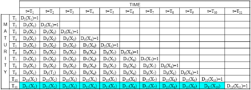
Figure 2.1: State variables we are interested in (N=10).

In conclusion, given a specified $X(t)$ process, we determine the functional forms of $D_{N+1}(X_{n})$ such that the model is calibrated to the market prices of European swaptions.

2.2.3 Black-Scholes Digital Mapping

Let’s illustrate the mapping from $X_{n}$ to $D_{N+1}(X_{n})$ assuming the terminal swap rate $S_{n}(T_{n})$ is lognormally distributed and thus smile is not taken into account. We conduct the mapping via Digital swaptions for the sake of its relatively simple payoff. This is why it’s called a ”Digital Mapping”. Because of the lognormal assumption above, the digital mapping here is call the ”Black-Scholes Digital Mapping”.

The functional form of the numeraire discount bond $D_{N+1}(X_{n})$ ($n=N,\ldots,1$) is determined by following a backward induction process from $T_{N}$ to $T_{1}$.

First the value at time 0 of a Digital Receiver Swaption with strike $K$ and maturity $T_{n}$, i.e., $DSN_{n}(0;K)$, is given by

$$DSN_{n}(0;K)=P_{n}(0)\Phi(\frac{\log(K/S_{n}(0))+\frac{1}{2}\bar{\sigma}_{n}^{2}T_{n}}{\bar{\sigma}_{n}\sqrt{T_{n}}}).$$ (2.18)

As explained in Appendix A.1 (see Equation A.11), Digital swaption values across a continuum of strikes imply the terminal density of the underlying swap rate. In the Black-Scholes world, this is assumed to be a lognormal distribution.

On the other hand, the option’s value can be expressed under the terminal measure $Q^{N+1}$ as

$$DSN_{n}(0;K)=D_{N+1}(0)\mathbb{E}_{0}^{N+1}[I_{\{S_{n}(X_{n})<K\}}\frac{P_{n}(X_{n})}{D_{N+1}(X_{n})}].$$ (2.19)

By Assumption 2 in Section 2.2.1, we have that $S_{n}(X_{n})$ is a strictly monotonically increasing function of $X_{n}$, which implies that we can invert the function to get a certain $x_{n}$ such that $\{S_{n}(X_{n})<K\}\Leftrightarrow\{X_{n}<x_{n}\}$. Thus $DSN_{n}(0;K)$ can be rewritten as

$$DSN_{n}(0;K)=D_{N+1}(0)\mathbb{E}_{0}^{N+1}[I_{\{X_{n}<x_{n}\}}\frac{P_{n}(X_{n})}{D_{N+1}(X_{n})}],$$ (2.20)

which we denote by a new symbol $\widetilde{DSN_{n}(0;x_{n})}$ instead of the original symbol $DSN_{n}(0;K)$. Applying the martingale property to $\frac{P_{n}(X_{n})}{D_{N+1}(X_{n})}$, we would get

$$\widetilde{DSN_{n}(0;x_{n})} = D_{N+1}(0)\mathbb{E}_{0}^{N+1}[I_{\{X_{n}<x_{n}\}}{E}_{T_{n}}^{N+1}[\frac{P_{n}(X_{n+1})}{D_{N+1}(X_{n+1})}]]$$ (2.21)

$$= D_{N+1}(0)\int_{-\infty}^{x_{n}}[\int_{-\infty}^{\infty}\frac{P_{n}(y)}{D_{N+1}(y)}\phi_{1}(y|z)dy]\phi_{2}(z)dz,$$

where $\phi_{1}$ denotes the probability density function of $X_{n+1}$ conditional on $X_{n}=x_{n}$ and $\phi_{2}$ denotes the probability density function of $X_{n}$. Note the functional form of $\frac{P_{n}(X_{n+1})}{D_{N+1}(X_{n+1})}$ can be determined by Equation A.3. Therefore $\widetilde{DSN_{n}(0;x_{n})}$ can be evaluated at least numerically for different values of $x_{n}$ which correspond to different values of K observed in the market.

Equating 2.18 and 2.21, we get

$$S_{n}(x_{n})=K=S_{n}(0)exp(-\frac{1}{2}\bar{\sigma}_{n}^{2}T_{n}+\bar{\sigma}_{n}\sqrt{T_{n}}\Phi^{-1}(\frac{\widetilde{DSN_{n}(0;x_{n})}}{P_{n}(0)})).$$ (2.22)

As $x_{n}$ is a certain value of $X_{n}$, we generalize Equation 2.22 to get the functional form of $S_{n}(X_{n})$.

$$S_{n}(X_{n})=S_{n}(0)exp(-\frac{1}{2}\bar{\sigma}_{n}^{2}T_{n}+\bar{\sigma}_{n}\sqrt{T_{n}}\Phi^{-1}(\frac{\widetilde{DSN_{n}(0;X_{n})}}{P_{n}(0)})).$$ (2.23)

Then the functional form of $D_{N+1}(X_{n})$ can be determined by rewriting Equation 2.16

$$D_{N+1}(X_{n})=\frac{1}{1+S_{n}(X_{n})\frac{P_{n}(X_{n})}{D_{N+1}(X_{n})}},$$ (2.24)

where $\frac{P_{n}(X_{n})}{D_{N+1}(X_{n})}$ has already been calculated in Equation 2.21.

2.2.4 Numerical Solution

In practice, the MF model is solved on a lattice. For each floating reset date $T_{n}$, we choose $2M+1$ values of $X_{n}$ from $-m\times\sigma_{X_{n}}$ to $m\times\sigma_{X_{n}}$, or equivalently $-M\times\Delta_{n}$ to $M\times\Delta_{n}$ with step length $\Delta_{n}$, see Figure 2.2, where

$$M = m\times(\mbox{number of steps in the interval length equal to one $\sigma_{X_{n}}$})$$

$$\Delta_{n} = \frac{\sigma_{X_{n}}}{\mbox{number of steps in the interval length equal to one $\sigma_{X_{n}}$}}$$

$$= \frac{\sqrt{\int_{0}^{T_{n}}\tau^{2}(u)du}}{\mbox{number of steps in the interval length equal to one $\sigma_{X_{n}}$}},$$

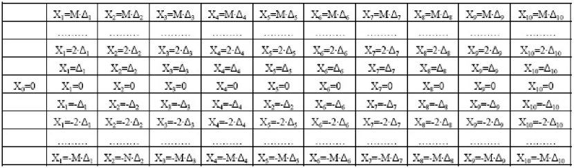
Figure 2.2: Lattice of $X_{n}$ (N=10).

An implementation of the MF model relies heavily on the evaluation of expectations using numerical integration routines. The numerical integration adopted was introduced by Pelsser [18], which is outlined as follows:

• fit a polynomial to the payoff function defined on the grid by applying Neville’s algorithm;

• calculate analytically the integral of the polynomial against the Gaussian distribution.

2.3 Volatility Function and Terminal Correlation

2.3.1 Volatility Function and Terminal Correlation

The prices of Bermudan swaptions depend strongly on the joint distribution or the terminal correlations of underlying swap rates $S_{n}(T_{n})$. By applying a first order Taylor expansion to $\log S_{n}(X_{n})$, we could get the following linear approximation. It it accurate enough for $X_{n}$ close to zero, where a majority of the probability mass concentrates.

$$\log S_{n}(T_{n},X_{n}) \approx \log S_{n}(T_{n},x)|_{x=0}+X_{n}\frac{\partial\log S_{n}(T_{n},x)}{\partial x}|_{x=0}$$ (2.26)

$$= \mbox{constant1}+\mbox{constant2}\times X_{n}.$$

Hence for $n<k$ we approximately have

$$Corr(\log S_{n}(T_{n}),\log S_{k}(T_{k}))\approx Corr(X_{n}(T_{n}),X_{k}(T_{k})).$$ (2.27)

The problem in turn transforms to finding the auto-correlation of the process $X(t)$. Pelsser [19] got inspired by the Hull-White model, whose short rate process $r(t)$ follows

$$dr(t)=(\theta(t)-ar(t))dt+\sigma dW(t).$$ (2.28)

By some algebra, we derive the auto-correlation structure of the short rates depending on the mean-reversion parameter $a$ via the relationship

$$Corr(r(t),r(s))=\begin{cases}\sqrt{\frac{t}{s}}&\mbox{if $a=0$}\\ \sqrt{\frac{e^{2at}-1}{e^{2as}-1}}&\mbox{if $a\neq 0$}\end{cases},$$ (2.29)

for $t<s$. If we set $X(t)$ process’ volatility function in equation 2.13 to be

$$\tau(t)=e^{at},$$ (2.30)

we would get an equivalent expression for the auto-correlation of the process $X(t)$

$$Corr(X(t),X(s))=\begin{cases}\sqrt{\frac{t}{s}}&\mbox{if $a=0$}\\ \sqrt{\frac{e^{2at}-1}{e^{2as}-1}}&\mbox{if $a\neq 0$}\end{cases},$$ (2.31)

for $t<s$. Thus, parameter $a$ can be interpreted as the mean-reversion parameter of the process $X(t)$. We can see from Equation 2.31 that increasing the mean-reversion parameter $a$ has the effect of reducing the auto-correlation between the values of $X(T_{n})$ for different floating reset dates $T_{n}$. Thus increasing the mean-reversion parameter reduces the auto-correlation between terminal swap rates $S_{n}(T_{n})$.

2.3.2 Estimation of the Mean-Reversion Parameter

Because of the ill-liquidity of other exotic interest rate derivatives that contain the information of terminal correlation of co-terminal swap rates, we are left with estimating the terminal correlations by historical data analysis. The correlation of $\log S_{n}(T_{n})$ and $\log S_{k}(T_{k})$, for $n<k$, is equivalent to the correlation of their log differences $\log\frac{S_{n}(T_{n})}{S_{n}(0)}$ and $\log\frac{S_{k}(T_{k})}{S_{k}(0)}$. This is because $S_{n}(0)$ and $S_{k}(0)$ are known today, division by which is sort of a normalization. One approach is to estimate the correlation by analyzing the most recently historical time series of $\log\frac{s_{t+T_{n}}(t+T_{n})}{s_{t+T_{n}}(t)}$ and $\log\frac{s_{t+T_{k}}(t+T_{k})}{s_{t+T_{k}}(t)}$. However, this method turns out to give estimates with large standard deviation due to the long lags needed for the calculation of the difference (see [16]). Therefore we instead analyze the time series with shorter lags, i.e., $\log\frac{s_{t+T_{n}}(t+\Delta u)}{s_{t+T_{n}}(t)}$ and $\log\frac{s_{t+T_{k}}(t+\Delta u)}{s_{t+T_{k}}(t)}$, where $\Delta u$ represents the lag size. If $\Delta u\rightarrow 0$, we are virtually analyzing the time series with infinitesimal lags, i.e., $d\log s_{t+T_{n}}(t+u)$ and $d\log s_{t+T_{k}}(t+u)$. If we stick to the lognormal assumption, i.e.,

$$\begin{cases}dS_{T_{n}}(u)=\sigma_{n}S_{T_{n}}(u)dW^{n,N+1}_{u}\\ dS_{T_{k}}(u)=\sigma_{k}S_{T_{k}}(u)dW^{k,N+1}_{u}\end{cases},$$ (2.32)

by applying It$\hat{o}$’s lemma we would have

$$\begin{cases}d\log S_{T_{n}}(u)=\sigma_{n}dW_{u}^{n,N+1}-\frac{1}{2}\sigma_{n}^{2}du\\ d\log S_{T_{k}}(u)=\sigma_{k}dW_{u}^{k,N+1}-\frac{1}{2}\sigma_{k}^{2}du\end{cases},$$ (2.33)

If we apply the Girsanov transformation, i.e., we set

$$\begin{cases}dW_{u}^{1}=dW_{u}^{n,N+1}-\frac{1}{2}\sigma_{n}du\\ dW_{u}^{2}=dW_{u}^{k,N+1}-\frac{1}{2}\sigma_{k}du\end{cases},$$ (2.34)

where $W_{u}^{1}$ and $W_{u}^{2}$ denote Brownian motions under the new measure, we would have

$$\begin{cases}d\log S_{T_{n}}(u)=\sigma_{n}dW_{u}^{1}\\ d\log S_{T_{k}}(u)=\sigma_{k}dW_{u}^{2}\end{cases}.$$ (2.35)

Let’s denote the instantaneous correlation between $W_{u}^{1}$ and $W_{u}^{2}$ by $\rho$, i.e.,

$$dW_{u}^{1}dW_{u}^{2}=\rho du.$$ (2.36)

Then the correlation we are interested in can be expressed as

$$Corr(\log\frac{S_{T_{n}}(T_{n})}{S_{n}(0)},\log\frac{S_{T_{k}}(T_{k})}{S_{k}(0)})=Corr(W_{u}^{1}(T_{n}),W_{u}^{2}(T_{k}))=\rho\sqrt{\frac{T_{n}}{T_{k}}}.$$ (2.37)

The problem thus transforms to a historical estimation of the instantaneous correlation $\rho$. In practice, we could approximately estimate $\rho$ by choosing a smallest possible lag size $\Delta u$, that is, one day. How valid this approach is depends on how valid the lognormal assumption is and how valid the approximation of instantaneous correlation by historically estimating the correlation on a daily basis is.

2.4 Bermudan Swaption Pricing under Markov-Functional

In this section, we first discuss the general backward induction method for valuing an American-style option, and then illustrate the pricing procedure under MF’s framework.

2.4.1 American-style Option Pricing in a Discrete Time Model

Let’s express everything in the swap/swaption context. Suppose we are under some risk-neutral measure Q with numeraire B(t) and the American swaption is allowed to exercise at any floating reset date $T_{n}(n=1,\ldots,N)$. Then the value of the American swaption $BSN(T_{n};K)$ at time $T_{n}$ can be computed backwardly as follows [24],

$$BSN(T_{N};K) = ESN_{N}(T_{N};K)$$

$$\frac{BSN(T_{n-1};K)}{B(T_{n-1})} = max\{\;\frac{ESN_{n-1}(T_{n-1};K)}{B(T_{n-1})}\;,\;\mathbb{E}_{T_{n-1}}^{Q}[\frac{BSN(T_{n};K)}{B(T_{n})}]\;\}$$ (2.38)

$$BSN(0;K) = B(0)\mathbb{E}_{T_{0}}^{Q}[\frac{BSN(T_{1};K)}{B(T_{1})}].$$

where the payoff of a European swaption at maturity $T_{n}$ is

$$ESN_{n}(T_{n};K)=max\{\;SV(T_{n};K)\;,\;0\},$$ (2.39)

where $SV(T_{n};K)$ is the swap value at time $T_{n}$ (see Section A.1 for notation).

2.4.2 Bermudan Swaption Pricing with the MF Model

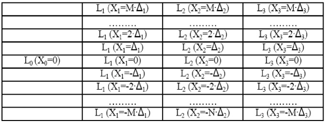
Figure 2.3: LIBOR ”tree” by MF model.

Assume N=4 and we have the LIBOR ”tree” after the digital mapping, shown in Figure 2.3, we can compute the corresponding swap value ”tree” and option valuation ”tree”, shown in Figure 2.4 and 2.5, respectively. In other words, we ought to determine the functional forms of $\frac{SV(X_{n};K)}{D_{N+1}(X_{n})}$ and $\frac{BSN(X_{n};K)}{D_{N+1}(X_{n})}$ so as to find out today’s option value $BSN(0;K)$.

Figure 2.4: Swap value ”tree” by MF model.

The functional form of numeraire-discounted swap value $\frac{SV(X_{n};K)}{D_{N+1}(X_{n})}$ can be determined by the backward induction:

$$\frac{SV(X_{N+1};K)}{D_{N+1}(T_{N+1})} = SV(X_{N+1};K)\;\;=\;\;\varphi[\alpha_{N}(r(X_{N})-K)]$$

$$\frac{SV(X_{n};K)}{D_{N+1}(X_{n})} = \mathbb{E}_{T_{n}}^{N+1}[\frac{SV(X_{n+1};K)}{D_{N+1}(X_{n})}]+\frac{\varphi[\alpha_{n-1}(r(X_{n-1})-K)]}{D_{N+1}(X_{n})}$$ (2.40)

$$\frac{SV(0;K)}{D_{N+1}(0)} = \mathbb{E}_{0}^{N+1}[\frac{SV(X_{1};K)}{D_{N+1}(X_{1})}],$$

where $\varphi$ is 1 for a payer swap and -1 for a receiver swap. Note there is no cash exchange at time $T_{1}$.

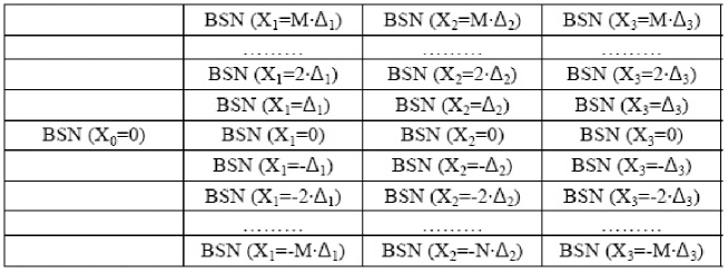
Figure 2.5: Option value ”tree” by MF model.

The functional form of numeraire-discounted option value $\frac{BSN(X_{n};K)}{D_{N+1}(X_{n})}$ can be determined backwards from $T_{N}$ to $T_{1}$:

If $T_{n}$ is not an exercise date, we have

$$\frac{BSN(X_{n};K)}{D_{N+1}(X_{n})}=\mathbb{E}_{T_{n}}^{N+1}[\frac{BSN(X_{n+1};K)}{D_{N+1}(X_{n+1})}].$$ (2.41)

If $T_{n}$ is an exercise date, we have

$$\frac{BSN(X_{n};K)}{D_{N+1}(X_{n})} = max\{\;\frac{ESN(X_{n};K)}{D_{N+1}(X_{n})}\;,\;\mathbb{E}_{T_{n}}^{N+1}[\frac{BSN(X_{n+1};K)}{D_{N+1}(X_{n+1})}]\;\}$$ (2.42)

$$= max\{\;max[\frac{SV(X_{n};K)}{D_{N+1}(X_{n})},0]\;,\;\mathbb{E}_{T_{n}}^{N+1}[\frac{BSN(X_{n+1};K)}{D_{N+1}(X_{n+1})}]\;\}$$

$$= max\{\;\frac{SV(X_{n};K)}{D_{N+1}(X_{n})}\;,\;\mathbb{E}_{T_{n}}^{N+1}[\frac{BSN(X_{n+1};K)}{D_{N+1}(X_{n+1})}]\;\},$$

where $BSN(X_{N+1};K)=0$.

Now we can obtain today’s Bermudan swaption value $BSN(0;K)$.

$$BSN(0;K)=D_{N+1}(0)\mathbb{E}_{0}^{N+1}[\frac{BSN(X_{1};K)}{D_{N+1}(X_{1})}].$$ (2.43)

Chapter 3 Integration of Volatility Smile

3.1 Incorporating Volatility Smile into the MF Model

In the MF model a smile can be incorporated quite naturally. What is required for this, is a model to obtain swaption prices across a continuum of strikes given a limited number of market quotes.

3.1.1 Interpolation of Implied Volatility

A first approach that might come into one’s mind is to keep the Black-Scholes mapping and interpolate/extrapolate the market quotes to obtain a continuum of implied volatilities as a function of the strike, i.e., $\bar{\sigma}_{n}(K)$. Then, provided that assumption 2 in Section 2.2.1 still holds, the only thing that we need to change in the mapping procedure described in Section 2.2.3, is to replace $\bar{\sigma}_{n}$ in Equation 2.23 with $\bar{\sigma}_{n}(S_{n}(X_{n}))$. More precisely, we instead solve numerically the following equation for $S_{n}(X_{n})$,

$$S_{n}(X_{n})=S_{n}(0)exp\{-\frac{1}{2}\bar{\sigma}_{n}^{2}(S_{n}(X_{n}))T_{n}+\bar{\sigma}_{n}(S_{n}(X_{n}))\sqrt{T_{n}}\Phi^{-1}(\frac{\widetilde{DSN_{n}(0;X_{n})}}{P_{n}(0)})\}.$$ (3.1)

In Ref. [14] a method is used for interpolation of the prices corresponding to the intermediate strikes such that the price of the ATM European swaption is preserved. However, as noted by Johnson [14] these smoothing methods may not satisfy the arbitrage-free constraints at all.

3.1.2 Uncertain Volatility Displaced Diffusion Model

An alternative approach is to base the digital mapping on an option pricing model that includes smile. In other words, we use another distribution rather than the lognormal one to approximate the terminal density of the swap rate, which allows for a good fit to the volatility smile observed in the market. In this project, we will use the Uncertain Volatility Displaced Diffusion model (hereafter UVDD) proposed by Brigo-Mercurio-Rapisarda [6].

In the following, we will first describe the displaced diffusion model which is the simplest extension of the lognormal model that can include skew effects. The description of the UVDD model will follow afterwards.

Displaced Diffusion Model (hereafter DD)

We assume in this setting that the dynamics of the swap rate $S_{n}(t)$ under the forward measure $Q^{n,N+1}$ is as follows,

$$dS_{n}(t)=\sigma_{n}(S_{n}(t)+m_{n})dW^{n,N+1}_{t}.$$ (3.2)

The parameter $m_{n}$ is called the displacement coefficient. Following the same reasoning from Equation A.6 to A.7, we can derive the closed form solution for the value of a Digital receiver swaption,

$$DSN_{n}(0;K)=P_{n}(0)\Phi(\frac{\log(\frac{K+m_{n}}{S_{n}(0)+m_{n}})+\frac{1}{2}\sigma_{n}^{2}T_{n}}{\sigma_{n}\sqrt{T_{n}}}).$$ (3.3)

Similarly, the value of a European swaption is given by

$$ESN_{n}(0;K) = \varphi P_{n}(0)((S_{n}(0)+m_{n})\Phi(\varphi d_{+})-(K+m_{n})\Phi(\varphi d_{-}))$$ (3.4)

$$d_{\pm} = \frac{\log(\frac{S_{n}(0)+m_{n}}{K+m_{n}})\pm\frac{1}{2}\sigma_{n}^{2}T_{n}}{\sigma_{n}\sqrt{T_{n}}},$$

where $\varphi$ is 1 for a payer European swaption and -1 for a receiver one.

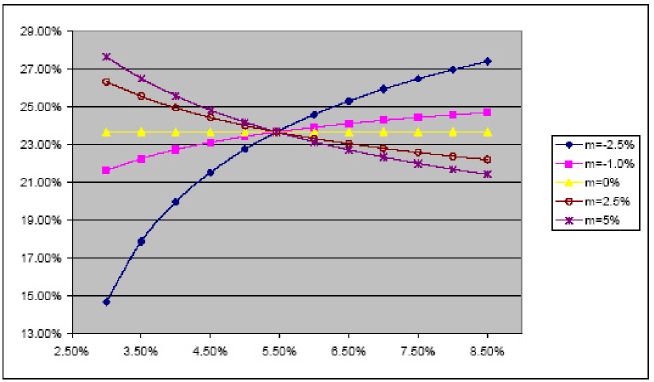
Figure 3.1: Implied skew for various values of the displacement coefficient.

The displacement coefficient can be used to generate an implied volatilities’ skew shape. A positive value of the displacement coefficient generates a downward sloping skew, while a negative value generates an upward slopping skew. The latter is unrealistic and should not be used. We report in Figure 3.1 the implied skew for various values of the displacement coefficient. The case $m_{n}=0\%$ corresponds to the usual lognormal model. We have used the market data corresponding to Data Set I in Appendix E.1.1 and Trade I in Appendix E.2. The tested instrument was a European swaption expiring at the fifth floating reset date, i.e., $T_{5}$, with at-the-money swap rate of $5.45\%$. The parameter $\sigma_{5}$ was adjusted such that the implied ATM volatility was the same for all cases. More precisely, we determine $\sigma_{5}$ such that the UVDD ATM price equals the BS ATM price.

The DD model can only incorporate the volatility skew, but market data suggest that the volatility quotes of swaption is typically a smile shape [9]. Thus the DD model is insufficient for describing the market quotes.

UVDD Model

In the UVDD setup, $S_{n}(t)+m_{n}$ is assumed to have the following dynamics

$$dS_{n}(t)=\begin{cases}\sigma_{n}^{0}(S_{n}(t)+m_{n})dW^{n,N+1}_{t}\;\;\;t\in[0,\varepsilon]\\ \eta_{n}(S_{n}(t)+m_{n})dW^{n,N+1}_{t}\;\;\;t>\varepsilon,\end{cases}$$ (3.5)

where $\sigma_{n}^{0}$ is a constant and $\eta_{n}$ is a random variable that is independent of $W^{n,N+1}_{t}$ and can take the following values,

$$\eta_{n}=\begin{cases}\sigma_{n}^{1}\;\;\;\mbox{with probability $\lambda_{n}^{1}$}\\ \sigma_{n}^{2}\;\;\;\mbox{with probability $\lambda_{n}^{2}$}\\ \vdots\\ \sigma_{n}^{M}\;\;\;\mbox{with probability $\lambda_{n}^{M}$}\end{cases},$$ (3.6)

where $\Sigma_{i=1}^{M}\lambda_{n}^{i}=1$. Denoting by $\mathbb{P}$ the risk neutral probability under the forward measure $Q^{n,N+1}$, we have

$$\mathbb{P}\{S_{n}(t)+m_{n}\leq y\}=\Sigma_{i=1}^{M}\mathbb{P}\{\{S_{n}(t)+m_{n}\leq y\}\cap\{\eta_{n}=\sigma_{n}^{i}\}\}=\Sigma_{i=1}^{M}\lambda^{i}\mathbb{P}\{S_{n}^{i}(t)+m_{n}\leq y|\eta_{n}=\sigma_{n}^{i}\},$$ (3.7)

Differentiating Equation 3.7 with respect to $y$, we get the probability density function of $S_{n}(t)+m_{n}$,

$$p_{n,t}(y)=\frac{\partial}{\partial y}\mathbb{P}\{S_{n}(t)+m_{n}\leq y\}=\Sigma_{i=1}^{M}\lambda_{n}^{i}\frac{\partial}{\partial y}\mathbb{P}\{S_{n}^{i}(t)+m_{n}\leq y|\eta_{n}=\sigma_{n}^{i}\}=\Sigma_{i=1}^{M}\lambda_{n}^{i}p_{n,t}^{i}(y),$$ (3.8)

where $p_{n,t}^{i}(y)$ is the density of a displaced lognormal variable with constant volatilities $\sigma_{n}^{i}$. The value of a Digital receiver swaption can be expressed under $Q^{n,N+1}$ as follows,

$$DSN_{n}(0;K) = P_{n}(0)\mathbb{E}_{0}^{n,N+1}[\frac{P_{n}(T_{n})I_{\{S_{n}(T_{n})<K\}}}{P_{n}(T_{n})}]$$ (3.9)

$$= P_{n}(0)\mathbb{E}_{0}^{n,N+1}[\frac{P_{n}(T_{n})I_{\{S_{n}(T_{n})+m_{n}<K+m_{n}\}}}{P_{n}(T_{n})}]$$

$$= P_{n}(0)\int_{0}^{+\infty}I_{\{y<K+m_{n}\}}\Sigma_{i=1}^{M}\lambda_{n}^{i}p_{n,t}^{i}(y)dy$$

$$= \Sigma_{i=1}^{M}\lambda_{n}^{i}P_{n}(0)\int_{0}^{+\infty}I_{\{y<K+m_{n}\}}p_{n,t}^{i}(y)dy$$

$$= \Sigma_{i=1}^{M}\lambda_{n}^{i}P_{n}(0)\mathbb{E}_{0}^{n,N+1}[I_{\{S_{n}^{i}(T_{n})+m_{n}<K+m_{n}\}}]$$

$$= \Sigma_{i=1}^{M}\lambda_{n}^{i}P_{n}(0)\mathbb{E}_{0}^{n,N+1}[I_{\{S_{n}^{i}(T_{n})<K\}}].$$

Now following once more the same line of reasoning from A.6 to A.7, we derive a closed form solution for the value of Digital receiver swaption,

$$DSN_{n}(0;K)=P_{n}(0)\Sigma_{i=1}^{M}\lambda_{n}^{i}\Phi(\frac{\log(\frac{K+m_{n}}{S_{n}(0)+m_{n}})+\frac{1}{2}(\sigma_{n}^{i})^{2}T_{n}}{\sigma_{n}^{i}\sqrt{T_{n}}}).$$ (3.10)

Similarly, the value of a European swaption can be determined analytically by

$$ESN_{n}(0;K) = \varphi P_{n}(0)\Sigma_{i=1}^{M}\lambda_{n}^{i}((S_{n}(0)+m_{n})\Phi(\varphi d_{+}^{i})-(K+m_{n})\Phi(\varphi d_{-}^{i}))$$ (3.11)

$$d_{\pm}^{i} = \frac{\log(\frac{S_{n}(0)+m_{n}}{K+m_{n}})\pm\frac{1}{2}(\sigma_{n}^{i})^{2}T_{n}}{\sigma_{n}^{i}\sqrt{T_{n}}},$$

where $\varphi$ is 1 for a payer European swaption and -1 for a receiver one.

We have performed the tests reported in this chapter with two components ($M=2$). The model can be expressed in terms of the following parameters $m_{n}$, $\sigma_{n}^{1}$, $\sigma_{n}^{2}$, $\lambda_{n}^{1}$, $\lambda_{n}^{2}$. It can be also expressed in terms of the parameters $m_{n}$, $\sigma_{n}$, $\omega_{n}$, $\lambda_{n}$ with:

$$\begin{cases}\sigma_{n}^{1}=\sigma_{n}\\ \sigma_{n}^{2}=\omega_{n}\sigma_{n}\\ \lambda_{n}^{1}=\lambda_{n}\\ \lambda_{n}^{2}=1-\lambda_{n}\end{cases}.$$ (3.12)

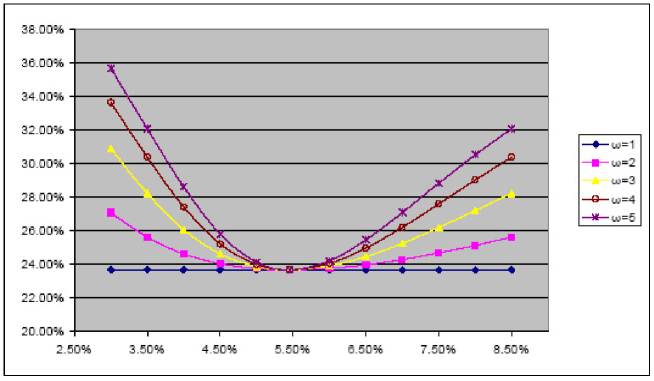
Figure 3.2: Implied smile by UVDD for various values of $\omega$ ($\lambda=0.75$, $m=0$).

We first report in Figure 3.2 the shapes of the volatility smile obtained by setting $\lambda_{n}$ to 0.75, $m_{n}$ to 0 and by varying $\omega_{n}$ from 1 to 5. The case $\omega_{n}=1$ reduces to the usual lognormal model. In this test and also the following one, we use the same data set and trade specification as was used in DD case described previously. We again adjust the parameter $\sigma_{5}$ such that the implied Black volatility corresponding to the at-the-money strike is the same for all the cases. We see that a mixture of lognormal components without displacement produces a symmetric smile centered around the at-the-money strike. The smile shape is more pronounced for higher values of $\omega_{5}$. This is because increasing the value of $\omega_{5}$ implies that there are fatter tails (both left side and right side) in the underlying distribution, and thus that away-from-the-money swaptions are more underpriced in a lognormal model.

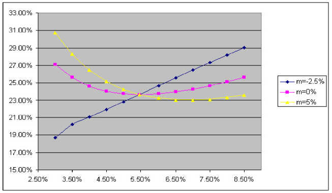
Figure 3.3: Implied smile by UVDD for various values of $m$ ($\lambda=0.75$, $\omega=2$).

We report in Figure 3.3 the shape of the volatility smile obtained by setting $\lambda_{5}$ to 0.75, $\omega_{5}$ to 2 and by varying $m_{5}$ from 1 to 5. When $m_{5}$ is set to zero, a symmetric smile is produced. Assigning a positive value to this parameter puts more weight on low strike and less weight on the high strike. The opposite happens when $m_{5}$ is set to a negative value. This is because a higher displacement implies a fatter left tail and a thinner right tail of the underlying distribution. Therefore, the UVDD approach allows for combining a symmetric shape of the smile with upward or downward sloping behavior.

3.1.3 UVDD Digital Mapping

We can perform the UVDD digital mapping by applying a small change in the original BS mapping. The BS mapping is explained in Section 2.2.3. In the UVDD digital mapping, the analytical formula for digital swaptions corresponding to the UVDD model (Equation 3.10) should be used instead of the Black digital formula. We get the functional form of $S_{n}(X_{n})$ by solving the following equation numerically with respect to $x_{n}$,

$$DSN_{n}(0;K) = DSN_{n}(0;S_{n}(x_{n}))$$ (3.13)

$$= P_{n}(0)\Sigma_{i=1}^{M}\lambda^{i}\Phi(\frac{\log(\frac{S_{n}(x_{n})+m_{n}}{S_{n}(0)+m_{n}})+\frac{1}{2}(\sigma_{n}^{i})^{2}T_{n}}{\sigma_{n}^{i}\sqrt{T_{n}}})$$

$$= \widetilde{DSN_{n}(0;x_{n})}.$$

Note that $\widetilde{DSN_{n}(0;x_{n})}$ is defined in Equation 2.21. This is a non-linear root-finding problem for which we resort to the Newton-Raphson method.

3.2 Test Results of Different Digital Mappings

We have performed a number of tests based on the market data of Data Set I in Appendix E.1 and using the setting of Trade I in Appendix E.2. The tests were run for the following digital mappings:

• case 1: a Black-Scholes mapping;

• case 2: a Displaced Diffusion mapping with $m_{n}=2.5\%$;

• case 3: a Displaced Diffusion mapping with $m_{n}=5\%$;

• case 4: a Displaced Diffusion mapping with $m_{n}=-2.5\%$;

• case 5: a UVDD mapping with $m_{n}=0\%$, $\lambda_{n}=0.75$ and $\omega_{n}=2$;

• case 6: a UVDD mapping with $m_{n}=0\%$, $\lambda_{n}=0.75$ and $\omega_{n}=5$;

• case 7: a UVDD mapping with $m_{n}=2.5\%$, $\lambda_{n}=0.75$ and $\omega_{n}=2$;

• case 8: a UVDD mapping with $m_{n}=2.5\%$, $\lambda_{n}=0.75$ and $\omega_{n}=3$.

For cases 2 to 8 we adjust the parameter $\sigma_{n}(n=1,2,\ldots,10)$ in order to recover the same ATM volatilities $\bar{\sigma}_{n}(n=1,2,\ldots,10)$ as for case 1. We first discuss the results obtained for some consistency checks. Next, some test results will be shown for the validity of the assumptions made in the MF model and the convergence of the Markov-Functional model with respect to the discretization parameters. Finally, we will discuss the effect of the smile on the value of Bermudan swaptions.

3.2.1 Consistency of European Swaption Prices

To demonstrate the correctness of the implementation, we first compare the European swaption values ($ESN_{n}$ for n=1..10) obtained by the MF model with the analytical formula for each of the eight cases mentioned above. The strike (fixed coupon rate) is set to 5$\%$. The results are shown in Table 3.1 to Table 3.4. The first row refers to the 1 into 10 period swaption and the last row to the 10 into 1 period swaption. The results clearly show that the MF model reproduces the values of the underlying Europeans with high accuracy: the relative error is less than 1 bp.

Analytical values	MF values
0.00	0.00
109.10	109.10
194.40	194.40
241.31	241.31
246.96	246.96
241.18	241.18
208.48	208.48
171.98	171.98
119.22	119.22
64.15	64.15

Table 3.1: Case 1 (Black-Scholes mapping).

Case 2		Case 3		Case 4
Analytical	MF values	Analytical	MF values	Analytical	MF values
0.00	0.00	0.00	0.00	0.00	0.00
107.86	107.86	107.25	107.25	113.05	113.05
194.79	194.79	194.98	194.98	193.26	193.26
243.10	243.10	244.01	244.01	236.28	236.28
249.43	249.43	250.70	250.70	240.23	240.23
244.12	244.12	245.67	245.67	233.35	233.35
211.25	211.25	212.72	212.72	201.21	201.20
174.52	174.52	175.88	175.88	165.46	165.46
121.07	121.07	122.05	122.05	114.54	114.54
65.21	65.21	65.79	65.79	61.52	61.52

Table 3.2: Case 2,3,4 (Displaced Diffusion mapping).

Case 5		Case 6
Analytical	MF values	Analytical	MF values
0.01	0.01	0.35	0.35
109.55	109.55	111.91	111.91
194.42	194.42	194.53	194.53
241.63	241.63	243.31	243.31
247.51	247.51	250.35	250.34
241.90	241.90	245.61	245.60
209.14	209.13	212.49	212.48
172.62	172.62	175.89	175.88
119.68	119.68	122.00	122.00
64.45	64.45	65.95	65.95

Table 3.3: Case 5,6 (UV mapping).

Case 7		Case 8
Analytical	MF values	Analytical	MF values
0.01	0.01	0.06	0.06
108.31	108.31	109.06	109.06
194.81	194.81	194.84	194.84
243.42	243.42	243.95	243.95
249.97	249.97	250.87	250.87
244.84	244.84	246.03	246.03
211.91	211.91	212.99	212.98
175.17	175.17	176.22	176.22
121.53	121.53	122.28	122.28
65.52	65.52	66.01	66.01

Table 3.4: Case 7,8 (UVDD mapping with $m=2.5\%$).

3.2.2 Convergence of the Numerical Algorithm

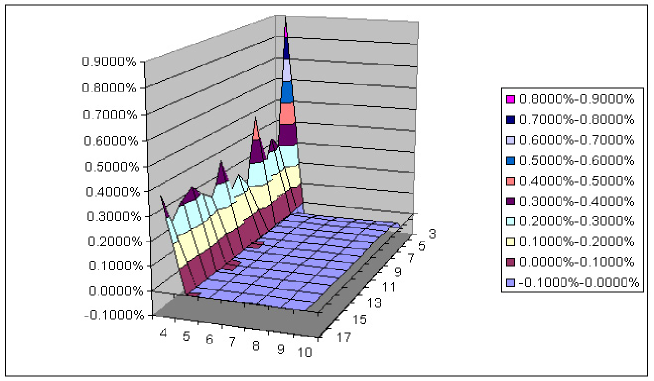
Figure 3.4: Relative pricing errors with respect to ”Steps per Deviation” and ”Number of Deviations”.

The MF model is based on a lattice. In this section, we check the convergence of the numerical integration with respect to the discretization of the lattice. There are two parameters controlling the level of discretization, namely,

• The range of values that $X$ can take expressed in units of its standard deviation, i.e. ”Number of Deviations”;

• The number of discrete points per standard deviation, i.e. ”Steps per Deviation”.

To access the convergence of the method, it is sufficient to look at the pricing of the European swaptions as this is basically exposed to the discretization error in the numerical integration. We consider the swaption which expires at $T_{7}$ and case 8 of Section 3.2.1. The analytical value of this European swaption is 212.986 bp. The relative error is shown in Figure 3.4, where the ”Steps per Deviation” ranges from 3 to 17 and the ”Number of Deviations” from 4 to 10. A very good convergence is obtained by using the following setting: ”Steps per Deviation” higher than 5 and ”Number of Deviations” higher than 4.

3.2.3 Assumption/Approximation Validity Check under UVDD Mapping

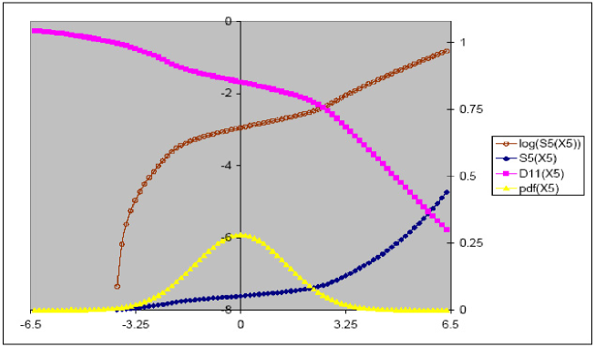
Figure 3.5: Assumption/Approximation validity check for $T_{5}$.

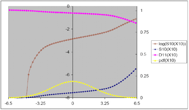
Figure 3.6: Assumption/Approximation validity check for $T_{10}$.

Before continuing further with pricing, we would like to check the validity of the assumptions made in Section 2.2.1. To summarize the following assumptions were made:

• The numeraire discount bond $D_{N+1}(t,X(t))$ is a function of $X(t)$;

• The terminal swap rate $S_{n}(T_{n},x)$ is a strictly monotonically increasing function of $x$.

In Figures 3.5 and 3.6, we show the functional behavior of $D_{N+1}(t,X(t))$ and $S_{n}(T_{n},X_{n})$, respectively, for $T_{5}$ and $T_{10}$ and corresponding to case 8. Also included in these figures is the probability density function of $X_{n}$. The following can be observed from these plots:

• The numeraire discount bond $D_{11}(X_{5})$ and $D_{11}(X_{10})$ are functions monotonically decreasing in $X_{5}$ and $X_{10}$, respectively;

• The swap rate $S_{5}(X_{5})$ and $S_{10}(X_{10})$, respectively, are functions strictly monotonically increasing in $X_{5}$ and $X_{10}$.

This demonstrates that the assumptions mentioned above are still valid for the UVDD mapping.

We would also like to check the linear approximation made in Equation 2.26 of Section 2.3.1. Here we repeat that equation below,

$$\log S_{n}(T_{n},X_{n}) \approx \log S_{n}(T_{n},x)|_{x=0}+X_{n}\frac{\partial\log S_{n}(T_{n},x)}{\partial x}|_{x=0}$$

$$= \mbox{constant1}+\mbox{constant2}\times X_{n}.$$

We report in Figure 3.5 and 3.6 the results for $T_{5}$ and $T_{10}$, respectively, and using the setting corresponding to case 8. We see that $\log S_{5}(X_{5})$ $\log S_{5}(X_{10})$ are linear functions of $X_{5}$ and $X_{10}$ for $X_{5}$ and $X_{10}$ close to zero. It should be noted that the approximation is even valid for the range of X where the majority of the probability mass is concentrated. This demonstrates that in the UVDD mapping the linear approximation is still valid.

3.2.4 Effect on Bermudan Swaption Prices

To test the impact of the shape of the implied volatility smile on the value of Bermudan swaptions, we consider the following trades and settings:

• A Bermudan swaption with the right to exercise at reset dates $T_{5}$, $T_{6}$, $T_{7}$, $T_{8}$, $T_{9}$ and $T_{10}$;

• All the different cases (case 4 eliminated) with the strike set to $3.5\%$, $5.5\%$ and $7.5\%$, respectively;

• Forward par swap rates $S_{5}(0)$, $S_{6}(0)$, $S_{7}(0)$, $S_{8}(0)$, $S_{9}(0)$ and $S_{10}(0)$ were set to $5.45\%$, $5.62\%$, $5.69\%$, $5.83\%$, $5.89\%$ and $6.06\%$, respectively. The mean-reversion parameter was set to $0\%$.

The results are reported in Table 3.5. Case 1 is the standard lognormal case.

Strike	3.50%	5.50%	7.50%
case 1	541.00	228.45	90.11
case 2	548.63	228.45	82.32
case 3	552.71	228.48	78.23
case 5	545.76	226.27	95.52
case 6	567.78	223.78	126.56
case 7	553.17	226.54	88.30
case 8	560.57	223.97	99.17

Table 3.5: Effect on the price of Bermudans.

For the displaced diffusion cases, i.e., cases 2-3, increasing the displacement coefficient leads to an increase in the implied volatilities corresponding to low strikes and to a decrease in the implied volatilities corresponding to high strikes. This results in a fatter left tail and a thinner right tail for the underlying’s distribution. Thus we see an increase in the displacement coefficient results in an increase in the value of a deep ITM Bermudan and a decrease in the value of a deep OTM Bermudan.

For the UVDD cases, i.e., cases 5-6 or 7-8, more pronounced smiles result in a higher price for a deep ITM/OTM Bermudan swaption. This can be explained in a similar way as above since a more pronounced smile leads to fatter tails (both left side and right side) in the distribution of the underlying. However, for the near-the-money Bermudans, we see that more pronounced smiles result in a lower price. This is counter-intuitive and is contrary to the findings of Abouchoukr [1]. We emphasize that the tests in that study were based on different market data and trade specifications. It was found that more pronounced smiles result in a higher near-the-money Bermudan price. To make sure that this result is not due to numerical artifacts, we have increased the ”Steps per Deviation” and ”Number of Deviations” to 100 and 20, respectively. The findings did not changed. A possible explanation for this phenomenon is provided in Appendix D. It is shown that this behavior is plausible in the case of a simple example.

In order to analyze the impact of the mean-reversion parameter, we valued the Bermudan swaption for case 1 and 8 for a wider range of strikes and two different mean-reversion levels ($0\%$ and $10\%$, respectively). The results are shown in Table 3.6. As expected, in both cases, the European value converges to the underlying swap value as the strike gets lower. Moreover, in both cases, the Bermudan swaption value converges to its European counterpart as the strike gets lower. This is because for a payer Bermudan it becomes more likely to exercise early as the strike gets lower.

To summarize the following can be concluded from the results presented in Table 3.6:

• Incorporating the volatility smile has a significant impact for the away-from-the-money Bermudan prices, while it has a relatively marginal impact for the near-the-money Bermudan prices. This is inline with the observation that the effect of smile on the Europeans is more pronounced as one moves away from the ATM level;

• For payer Bermudans, increasing the mean-reversion level gives rise to an increase of the overall level of Bermudan prices. This can be roughly explained as follows. Increasing the mean-reversion level will reduce the terminal correlations of swap rates $S_{n}(T_{n})$ and $S_{k}(T_{k})$ for $n=1..N,k>n$ (see Section 2.3.1). In our case, if in the future state at $T_{5}$, $S_{5}(T_{5})$ was below the strike, a higher mean-reversion level would increase the likelihood that the economy would transform to a state at a further future time $T_{n}$ for $n=6,7,8,9,10$ in which $S_{n}(T_{n})$ would be higher than the strike, and thus increasing the value of the Bermudan.

  Finally, the increase is more pronounced for the near-the-money Bermudans compared to the away-from-the-money ones. This can be explained as follows. If the strike is much lower than the ATM level, the Bermudan will be less sensitive to the terminal correlations as the likelihood of early exercising at $T_{5}$ is quite high. If the strike gets much higher than the ATM strike level, this effect would become less pronounced too as the likelihood of postponing the exercise later in future will increase.

Strike	3.00%	3.50%	4.00%	4.50%	5.00%	5.50%
Swap value	639.98	509.63	379.28	248.93	118.58	-11.77
European (BS)	645.22	526.08	418.22	324.74	246.96	184.52
Bermudan MR=0% (BS)	652.52	541.00	442.23	357.49	286.60	228.45
Bermudan MR=10% (BS)	656.70	547.48	450.62	367.07	296.63	238.30
Bermudan MR=0% (UVDD)	675.22	560.57	455.04	362.39	285.15	223.97
Bermudan MR=10% (UVDD)	679.24	565.75	461.58	370.09	293.51	232.50
European (UVDD)	663.95	546.10	435.07	335.24	250.87	184.29
Strike	6.00%	6.50%	7.00%	7.50%	8.00%	8.50%
Swap value	-142.12	-272.47	-402.82	-533.17	-663.52	-793.87
European (BS)	135.85	98.84	71.23	50.95	36.24	25.67
Bermudan MR=0% (BS)	181.41	143.75	113.81	90.11	71.40	56.65
Bermudan MR=10% (BS)	190.64	152.11	121.18	96.49	76.83	61.23
Bermudan MR=0% (UVDD)	177.84	143.48	118.04	99.17	84.85	73.67
Bermudan MR=10% (UVDD)	186.11	151.38	125.55	106.23	91.43	79.80
European (UVDD)	135.00	100.33	76.63	60.49	49.23	41.02
MR denotes the mean-reversion level.

Table 3.6: Bermudan prices for a wider range of strikes (case 1 and 8).

Chapter 4 Future Smile and Smile Dynamics

4.1 Future Volatility Smile Implied by MF Models

It is well-known that the value of a path dependent option is highly sensitive to the future volatility smile (see e.g. Ayache [2] and Rosien [22]). The future volatility smile is defined as follows. Today we observe market quotes $\sigma_{n}(K)$ for European swaptions expiring at $T_{n}$. We calibrate our model to the vanilla options such that the terminal density of the underlying is consistent with the market. We now move to a future date which is still before expiry, and use our calibrated model to compute, at that time, values of the vanilla options across strikes. Conditional on the state of the future date, we can invert the option values to get the implied smile, i.e. the future volatility smile. It should be noted that in the MF model the state transition is controlled by the mean-reversion parameter.

Let’s now explain in more detail how to obtain future smiles in the MF models. For ease of calculation, we choose the future date, denoted by $T_{f}$, to be one of the floating reset dates, i.e., $T_{f}=T_{m}$ for $m=1,2,\ldots,N-1$. Suppose at time $T_{f}$, $X_{f}=x_{f}$. Conditional on this state, the value of the European swaption is determined as described in Section 2.4.2. In order to get the implied volatility from the price, we still need to determine $P_{n}(x_{f})$ and $S_{n}(x_{f})$. This can be done by using the functional form of $D_{k}(x_{f})$ (k=n,..,N+1) which can be obtained through numerical integration on the calibrated lattice. For more details we refer to Section 2.2.2. Note that all these computations depend on the conditional expectation $\phi(X_{k}|X_{i})$, for $k>i$ and $i=f,f+1,\cdots,N$, which is ultimately subject to the mean-reversion parameter value.

4.1.1 Future Volatility Smile Implied by the BS Mapping

We first investigate the future volatility smile implied by the Black-Scholes digital mapping, i.e., the future volatility smile implied by case 1 in Section 3.2. The test was run for a payer swaption expiring at the seventh floating reset date, i.e., $T_{7}$. The at-the-money swap rate $S_{7}(0)$ was around $5.69\%$, and the mean-reversion parameter was set to zero. We calculated the future smiles standing at $T_{3}$ conditional on different future states $X_{3}$ such that the underlying swap rate $S_{7}(x_{3})$ ranges from $4.92\%$ to $6.21\%$. The corresponding future smiles are reported in Figure 4.1. In the case of the Black-Scholes model we expect the future smile to be flat. We see that this is not the case in the MF model with the BS mapping. However, the future smiles obtained for the different strikes (low and high, respectively) are compensating each other. More precisely, the fat-tailed distributions implied for high swap rates compensate the thin-tailed distributions implied for low swap rates. Therefore, on an integrated level we still may obtain a flat smile.

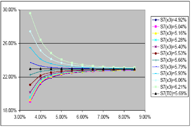
Figure 4.1: Future smiles implied by BS mapping and today’s flat volatility.

4.1.2 Future Volatility Smile Implied by the UVDD Mapping

We will now investigate the future volatility smile implied by the UVDD digital mapping, more precisely, the future volatility smile implied by case 8 in Section 3.2. The test was run for a payer swaption expiring at the ninth floating reset date, i.e., $T_{9}$. The at-the-money swap rate $S_{9}(0)$ was $5.89\%$. We calculated the future smiles standing at $T_{6}$. We adjusted $X_{6}$’s value such that the underlying swap rate $S_{9}(x_{6})$ varies approximately from $4.8\%$ to $6.5\%$. In order to study the effect of the mean-reversion parameter, we considered three MR levels, namely $0\%$, $10\%$, and $30\%$, respectively. The results of these three tests together with today’s smile are reported in Figure 4.2, 4.3 and 4.4, respectively. We see that increasing the mean-reversion level has the effect of increasing the overall level of the future smiles. This can be explained as follows. For $X_{f}$ close to zero, $S_{n}(T_{f},X_{f})$, can be approximated as follows,

$$S_{n}(T_{f},X_{f}) \approx S_{n}(T_{f},x)|_{x=0}+X(T_{f})\frac{\partial S_{n}(T_{f},x)}{\partial x}|_{x=0}$$ (4.1)

$$= \mbox{constant1}+\mbox{constant2}\times X(T_{f}).$$

The correlation between the future underlying level $S_{n}(T_{f},X_{f})$ and the terminal underlying level $S_{n}(T_{n},X_{n})$ is given by,

$$Corr(S_{n}(T_{f}),S_{n}(T_{n}))\approx\rho(X_{f}(T_{f}),X_{n}(T_{n}))=\begin{cases}\sqrt{\frac{T_{f}}{T_{n}}}&\mbox{if $a=0$}\\ \sqrt{\frac{e^{2aT_{f}}-1}{e^{2aT_{n}}-1}}&\mbox{if $a\neq 0$}\end{cases}.$$ (4.2)

Here we use the analytical form of $Corr(X_{f}(T_{f}),X_{n}(T_{n}))$ from Section 2.3.1, and $a$ is the mean-reversion parameter. Therefore, increasing the mean-reversion parameter $a$ has the effect of reducing the correlation between the future underlying level $S_{n}(T_{f},X_{f})$ and the terminal underlying level $S_{n}(T_{n},X_{n})$. This implies that the average volatility within the time period $[T_{f},T_{n}]$ increases, which is consistent with the phenomenon we observe in Figure 4.2, 4.3 and 4.4.

In conclusion, by calibrating the mean-reversion parameter to the relevant market information, the MF model is able to control the future smiles to some extent.

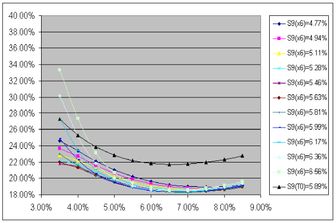
Figure 4.2: Future smiles implied by UVDD mapping for $MR=0\%$ and today’s smile.

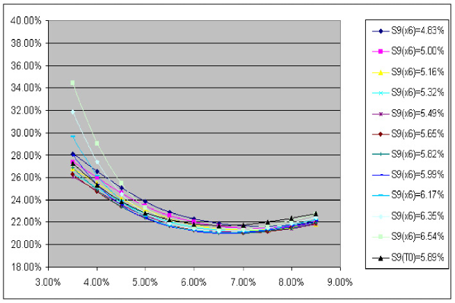
Figure 4.3: Future smiles implied by UVDD mapping for $MR=10\%$ and today’s smile.

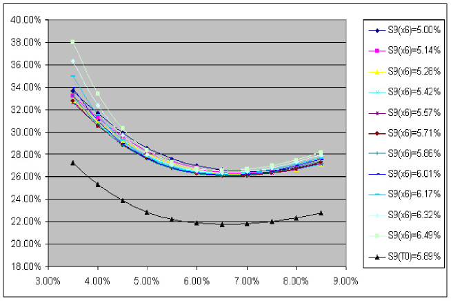
Figure 4.4: Future smiles implied by UVDD mapping for $MR=30\%$ and today’s smile.

4.2 Smile Dynamics Implied by the UVDD Model

Many previous studies [2][9][22][25] point out that the smile dynamics implied by an option pricing model indicates whether the model is able to produce good hedge ratios. Let’s take a look at an European option and a model $M$. We define the implied volatility, $\sigma_{imp}(S;K,T)$, as the volatility that should be used in the Black model to match the value of this option obtained using model $M$,

$$V(S;K,T)=V_{BS}(S,\sigma_{imp}(S;K,T);K,T),$$ (4.3)

where $V(S;K,T)$ denotes the value of the European option as obtained by model $M$. By Equation 4.3, we can obtain the implied Black volatility $\sigma_{imp}(S;K,T)$, which is a function of the underlying $S$ with parameters strike $K$ and maturity $T$, from the prices implied by the model.

The delta hedge ratio of this model, $\Delta(S;K,T)$, is given by,

$$\Delta(S;K,T) = \frac{\partial V(S;K,T)}{\partial S}\;\;\;=\;\;\;\frac{\partial V_{BS}(S,\sigma_{imp}(S;K,T);K,T)}{\partial S}$$ (4.4)

$$+ \frac{\partial V_{BS}(S,\sigma_{imp}(S;K,T);K,T)}{\partial\sigma_{imp}(S;K,T)}\times\frac{\partial\sigma_{imp}(S;K,T)}{\partial S}.$$

From Equation 4.4, we see that the validity of the delta ratio generated by model $M$ is subject to the sensitivity $\frac{\partial\sigma_{imp}(S;K,T)}{\partial S}$. This is what we mean by the smile dynamics of a model. In Ayache [2] and Rosien [22], they entitle a wider concept to smile dynamics, which also covers the structure of conditionals apart from this sensitivity. In our report, we stick to this definition of the smile dynamics, i.e.,

$$\mbox{Smile Dynamics}\;\;\triangleq\;\;\frac{\partial\sigma_{imp}(S;K,T)}{\partial S}.$$ (4.5)

The smile dynamics has been a point of discussion for many models. It is well-known that the stochastic volatility models show a sticky delta behavior, while local volatilty models may predict the opposite smile dynamics [9]. To study the smile dynamics of the UVDD model, we have calculated the smile dynamics by the following cases:

• We first considered a digital mapping corresponding to case 6 of Section 3.2, i.e., the model has no displacement but is a purely Uncertain Volatility (UV) model. Moreover, a swaption expiring at the fifth floating reset date, i.e., $T_{5}$, with at-the-money swap rate of $5.45\%$ was considered. The first experiment was done by bumping up/down the yield curve by 50 bp so that the underlying swap rate $S_{5}(0)$ increases/decreases to $5.73\%/5.17\%$, respectively. We use the calibrated UV model corresponding to the un-bumped case. The volatility smiles are shown in Figure 4.5. We observe a sticky delta smile dynamics. This is not surprising as the UV model falls into the category of stochastic volatility models, whose smile dynamics has typically a sticky delta effect [22];

• Because bumping the yield curve also changes the PVBP, $P_{5}(0)$, (see Equation A.9), in the second experiment, we have bumped up/down only the discount factor $D_{5}(0)$ by an amount of 100 bp so that only $S_{5}(0)$ increases/dereases to $5.84\%/5.07\%$ while $P_{5}(0)$ retains at the original level. The implied volatility smiles are reported in Figure 4.6. We observe the same sticky delta phenomenon as was obtained in the first experiment.

Figure 4.5: Smile dynamics implied by the UV model by bumping the yield curve.

Figure 4.6: Smile dynamics implied by UV by bumping only the discount factor $D_{5}(0)$.

We repeated these two experiments for case 8 in Section 3.2, i.e., the UVDD model. The corresponding results are shown in Figure 4.7 and 4.8, respectively. In both figures, we see the ATM implied volatility is sloping down and the smile moves in the same direction as the underlying’s movement. This is qualitatively consistent with the market observation according to Hagan [9].

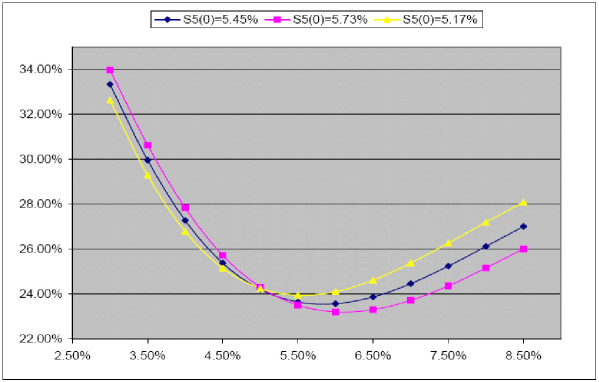
Figure 4.7: Smile dynamics implied by the UVDD model by bumping the yield curve.

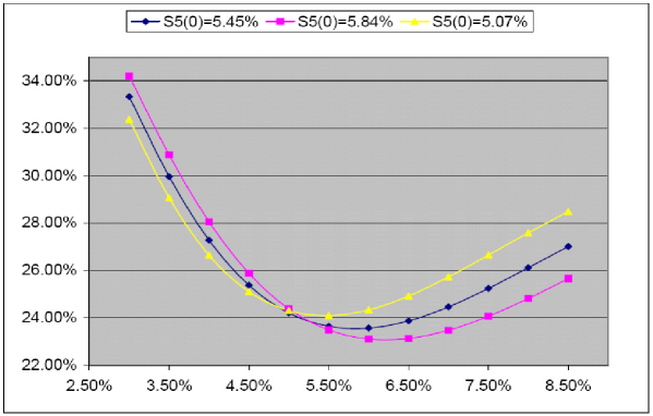
Figure 4.8: Smile dynamics implied by UVDD by bumping only the discount factor $D_{5}(0)$.

Chapter 5 Calibration of UVDD Model

In this section, we will first discuss the different choices that can be made in the calibration procedure, namely: minimization of the error in terms of option prices or in terms of implied volatilities. Next, we will discuss the results that have been obtained using different settings in the calibration procedure.

5.1 Calibration Methods

We may calibrate the UVDD model by minimizing the error in terms of option prices (OP) across $L$ strikes, that is,

$$\begin{cases}\mbox{minimizing}\;\;F(\overrightarrow{y})=\frac{1}{L}\Sigma_{i=1}^{L}(ERR_{OP}(K_{i};\overrightarrow{y}))^{2}\\ \mbox{subject to}\;\begin{cases}\lambda^{j}\in[0,1]\;\mbox{for}\;j=1,\cdots,M\;\mbox{and}\;\Sigma_{j=1}^{M}\lambda^{j}=1\\ \sigma^{j}>0\;\mbox{for}\;j=1,\cdots,M\end{cases},\end{cases}$$ (5.1)

where

$$\begin{cases}ERR_{OP}(K_{i};\overrightarrow{y})\triangleq\frac{OP^{model}(K_{i};\overrightarrow{y})-OP^{market}(K_{i})}{OP^{market}(K_{i})}\\ \overrightarrow{y}\triangleq[m,\lambda^{1},\sigma^{1},\lambda^{2},\sigma^{2},\cdots,\lambda^{M},\sigma^{M}]\end{cases}.$$ (5.2)

Alternatively, we may instead minimize the error in terms of implied volatilities (IV), that is,

$$\begin{cases}\mbox{minimizing}\;\;F(\overrightarrow{y})=\frac{1}{L}\Sigma_{i=1}^{L}(ERR_{IV}(K_{i};\overrightarrow{y}))^{2}\\ \mbox{subject to}\;\begin{cases}\lambda^{j}\in[0,1]\;\mbox{for}\;j=1,\cdots,M\;\mbox{and}\;\Sigma_{j=1}^{M}\lambda^{j}=1\\ \sigma^{j}>0\;\mbox{for}\;j=1,\cdots,M\end{cases}\end{cases},$$ (5.3)

where

$$ERR_{IV}(K_{i};\overrightarrow{y})\triangleq\frac{IV^{model}(K_{i};\overrightarrow{y})-IV^{market}(K_{i})}{IV^{market}(K_{i})}.$$ (5.4)

However, in practice, solving the first optimization problem does not mean that we have an optimal solution for the other, and vice versa. We will explain this below. Due to the relationship,

$$\frac{\Delta OP(K_{i};\overrightarrow{y})}{\Delta IV(K_{i};\overrightarrow{y})}\approx Vega(K_{i}),$$ (5.5)

we can derive the following relation after some algebraic manipulations,

$$ERR_{IV}(K_{i};\overrightarrow{y})\approx\frac{OP^{market}(K_{i})\times IV^{market}(K_{i})}{Vega(K_{i})}\times ERR_{OP}(K_{i};\overrightarrow{y}).$$ (5.6)

First note that $IV^{market}(K_{i})$ stays in a relatively narrow range across strikes, while $OP^{market}(K_{i})$ and $Vega(K_{i})$ may vary widely subject to the strike $K_{i}$. If $OP^{market}(K_{i})$ is very big or $Vega(K_{i})$ is very small, $ERR_{IV}(K_{i};\overrightarrow{y})$ can still be large even for very small values of $ERR_{OP}(K_{i};\overrightarrow{y})$. It will be the other way around if $OP^{market}(K_{i})$ is very small or $Vega(K_{i})$ is very big. This means that in practice, it is very difficult to satisfy both criteria simultaneously.

We choose to minimize the error in terms of option prices instead of implied volatilities because of the following reasons:

• We want to get a consistent terminal density of the underlying by the calibration procedure. The implied density is directly sensitive to the accuracy in terms of option prices (see Equation A.11). On the other hand, by Equation A.11, we may have

  $$\phi(K)=\frac{\partial\widetilde{DSN_{n}(t;\sigma_{imp}(K))}}{\partial\sigma_{imp}(K)}\frac{\partial\sigma_{imp}(K)}{\partial K}$$ (5.7)

  Please note that $\frac{\partial\sigma_{imp}(K)}{\partial K}$ is directly sensitive to the accuracy in terms of implied volatilities. This means that a small minimization error in terms of implied volatilities may lead to a large error in the value of $\phi(K)$ because of a high vega level.

• Computing $OP^{market}(K_{i})$ is much faster compared to computing $IV^{market}(K_{i})$. This is because for the latter we have to include an extra step in the minimization procedure, in which the implied volatility is obtained from the option price.
  

In the calibration we use only two components for the UVDD model, i.e., $M=2$, and thus we can alternatively use the parametric scheme described in Equation 3.12. We do this because of the following reasons:

• If $M=2$, every parameter plays a clear role: $\sigma$ controls the level of the smile/skew; $m$ controls the implied volatilities’ skewness; $\omega$ and $\lambda$ are responsible for the convexity, i.e., the shape of the smile. But if $M>2$, the interpretation for each parameter is not that clear any more;

• As we will see in the next section, a mixture of two lognormal distributions is rich enough for fitting the market prices.

Furthermore, in the calibration, we fix $\lambda$ and thus have only three free parameters ($\sigma^{1}$, $\sigma_{2}=\omega\sigma^{1}$ and $m$). We may do this because $\omega$ and $\lambda$ control similar features of the implied volatilities.

Now the calibration problem reduces to

$$\begin{cases}\mbox{minimizing}\;\;F(\overrightarrow{y})=\frac{1}{L}\Sigma_{i=1}^{L}(ERR_{OP}(K_{i};\overrightarrow{y}))^{2}\\ \mbox{subject to}\;\;\;\sigma^{1}>0,\sigma^{2}>0\;\mbox{and}\;m\geq 0\end{cases},$$ (5.8)

where

$$\overrightarrow{y}\triangleq[\sigma^{1},\sigma^{2},m].$$ (5.9)

We set $m\geq 0$ because the case of $m<0$ would generate an unrealistic shape of implied volatilities.

We are using the NL2SOL minimizer in the calibration. NL2SOL is an unconstrained minimizer. Thus we need to transform our bounded model parameters to unbounded ones:

$$x = \log(\sigma^{1})$$ (5.10)

$$y = \log(\sigma^{2})$$ (5.11)

$$z = \log{(\frac{h_{m}}{m}-1)}.$$ (5.12)

Equation 5.12 is just for restricting $m$ within $(0,h_{m})$. This will be used in Section 5.2 (case 6).

5.2 Calibration Results

We run our tests based on the market data corresponding to Data Set II in Appendix E.1.2, which is for the EURO market, and used the setting of Trade II in Appendix E.2. We calibrate the following models to all co-terminal swaptions, $ESN_{n}$ for n=1,..,20:

• case 1: a Black model, that is, we take the ATM quote as the flat volatility. This case serves as a benchmark for the relative error when smile is not taken into account;

• case 2: a lognormal model, that is, a reduced Displaced Diffusion model with $m_{n}=0$. In this case, we are not necessary fitting the ATM volatility;

• case 3: a Displaced Diffusion model with $m_{n}\geq 0$;

• case 4: a UVDD model for $m_{n}\geq 0$ and $\lambda_{n}=0.75$;

• case 5: the same model as in case 4, but the calibration is done in terms of implied volatilities instead of options prices;

• case 6: a UVDD model for $0\leq m_{n}\leq 0.10$ and $\lambda_{n}=0.75$.

For each option maturity $T_{i}$ $(i=1,2,\cdots,20)$, we calibrate the model to market prices for strikes where the offset relative to the ATM point varies from -100bp to 100bp, in total 9 quotes. These 20 input volatility skews/smiles are shown in Figure 5.1. The relative error for the calibration of the above models in terms of option prices is shown from Figure 5.2 to 5.7, respectively. The average absolute error is also listed in the legend of each figure.

From Figure 5.2 to 5.4, we see that the Displaced Diffusion model improves the fitting to market prices significantly than the Black model. From Figure 5.4 and 5.5, we see that the UVDD model further improves the fitting to market prices significantly than the Displaced Diffusion model. In this test, we don’t see from Figure 5.5 and 5.6 any difference between the calibrations in terms of option prices and implied volatilities. A comparison for the relative error in all the cases is shown in Figure 5.8.

Sometimes, if we want to get a very good fit to the market, the calibrated $m_{n}$ parameter can be extremely large, for instance, more than 100, and in the same time the calibrated $\sigma_{n}^{1}$ and $\sigma_{n}^{2}$ can be extremely small, for instance, less than 0.01bp. $m_{n}$ being 100 means that a negative swap rate very close to -10000% is allowed in the model, which is obviously unrealistic. Therefore, we prefer a local solution which leads to realistic parameters over a global solution which may be unrealistic. This is why we have restricted the displacement parameter in case 6. We see in Figure 5.7 that restricting $m_{n}$ within $(0,0.10)$ still gives us a reasonably good fit.

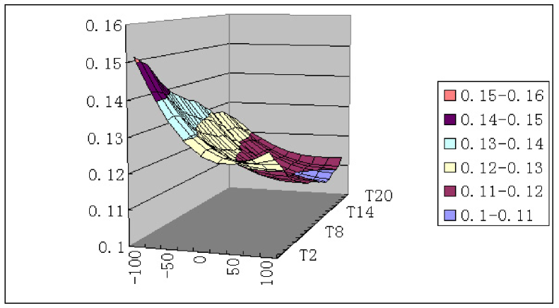
Figure 5.1: Input volatility surface.

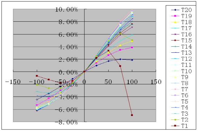
Figure 5.2: Relative error across strike obtained for the Black model with ATM volality in terms of option prices; the average absolute error is 3.93%.

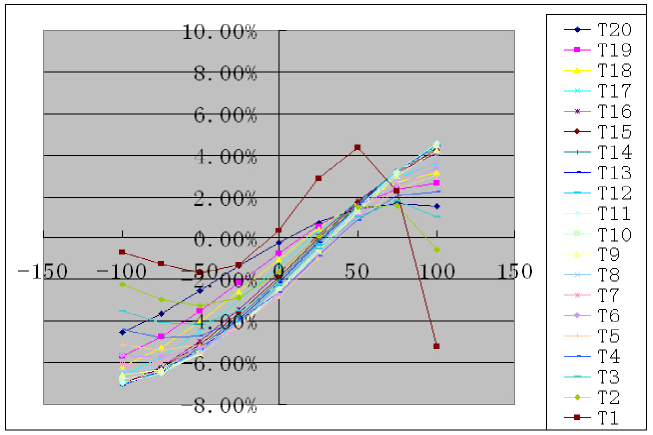
Figure 5.3: Relative error across strike obtained for the calibration of the lognormal model in terms of option prices; the average absolute error is 3.26%.

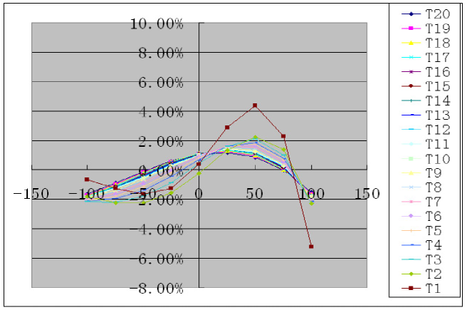
Figure 5.4: Relative error across strike obtained for the calibration of the Displaced Diffusion model in terms of option prices; the average absolute error is 1.22%.

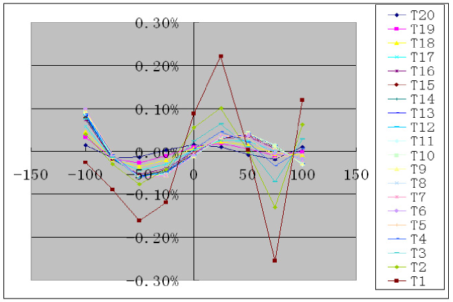
Figure 5.5: Relative error across strike obtained for the calibration of the UVDD model in terms of option prices; the absolute absolute error is 0.04%.

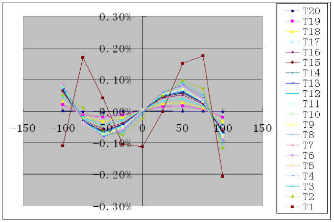
Figure 5.6: Relative error across strike obtained for the calibration of the UVDD model in terms of implied volatilities; the absolute absolute error is 0.05%.

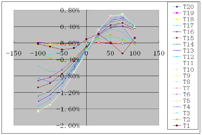
Figure 5.7: Relative error across strike obtained for the calibration of the UVDD model with $m_{n}$ within $(0,0.10)$ in terms of option prices; the average absolute error is 0.49%.

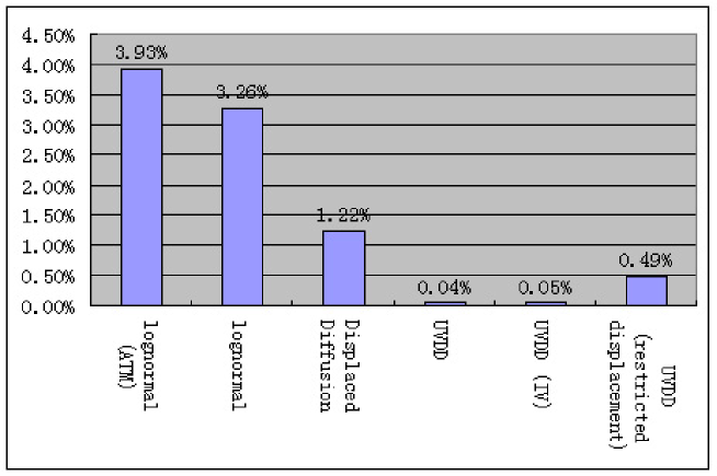
Figure 5.8: Comparison of average absolute error for all the cases.

5.3 Terminal Density Implied by the UVDD Model

Another interesting quantity is the terminal density implied by the model for the underlying swap rate. We study this for the underlying rate with maturity at $T_{18}$ corresponding to case 4 of Section 5.2. The input implied volatility quotes are shown in Figure 5.9. The ATM strike level is $4.75\%$. The probability density function is plotted in Figure 5.10, and the calibrated model parameters are listed below.

$$\begin{cases}\sigma_{18}^{1}=2.45\%\\ \sigma_{18}^{2}=8.79\%\\ m_{18}=8.52\%\end{cases}.$$

In Figure 5.10, the implied distribution by taking only the ATM volatility, i.e., the counterpart lognormal distribution, is plotted as well. We see that the UVDD model allows for negative swap rates (down to almost $-8.79\%$) which is unrealistic. However the negative swap rates have small densities ($Prob(S_{18}(T_{18})\leq 0)=3.95\%$). Such a small fraction of negative swap rates leads to a left-side fat tail, and thus helps the model to generate the skew effect. Figure 5.11 shows the two lognormal components of the implied distribution, each of them scaled by their weight factor.

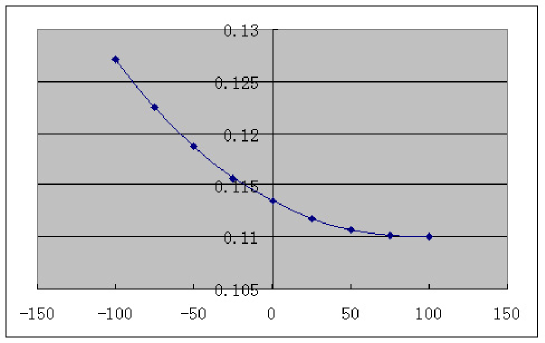
Figure 5.9: Implied volatility smile for $T_{18}$.

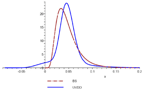
Figure 5.10: Probability densities of the swap rate $S_{18}(T_{18})$.

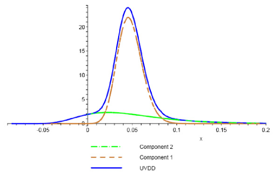
Figure 5.11: Decomposition of the probability density function for $S_{18}(T_{18})$.

Chapter 6 Hedging Simulations

6.1 Overview of the Hedging Simulations

We have performed our hedging simulations on a 10 year Bermudan swaption with the right to exercise at floating reset dates $T_{n}$, for $n=1,2,\cdots,10$. The trade is running from May 28th 2004 to July 29th 2005 (in total 14 months). The trade specification is shown in Table E.6 of Appendix E.2. The market data for the hedge tests, part of which was created synthetically based on the available data, is presented in Section 6.2. We have performed both delta and delta+vega hedgings to the smile and non-smile Bermudans. The details of the hedging strategies will be explained in Section 6.3. The calculation of delta and vega ratios will be elaborated in Section 6.4. Below we summarize the most important conclusions from the conducted hedging simulations:

• The smile model outperforms the non-smile model in both delta hedging and delta+vega hedging simulations. In both the smile and non-smile cases, a delta hedging reduces the profit$\&$loss effect of the unhedged Bermudan trade significantly, and a delta+vega hedging further improves the delta hedging performance significantly. Besides, a delta+vega hedging reduces significantly the oscillation of the hedged NPV compared to the corresponding delta hedging, but doesn’t affect the drift level of the hedged NPV. The above conclusions will be drawn gradually from Section 6.5.1 to 6.5.3;

• The change from rolling the vega positions from daily to monthly has little impact on the delta+vega hedged NPV. The relevant details can be found in Section 6.5.1;

• Increasing the mean-reversion parameter reduces the drift of the hedged NPV, but doesn’t affect its oscillation. The relevant details are in Section 6.5.4.

6.2 Market and Synthetic Data

6.2.1 Available Market Data

Yield Curve Data

There are two kinds of yield curve related data. The first one is the deposit rates of 2 days, 1 week, 1 month, 2 months, 3 months, 6 months and 9 months, all shown in Figure 6.1. The second one is the spot-starting swap rates with tenors from 1 year to 15 years, shown in Figure 6.2. The deposit rates are used to construct the short-end of the yield curve. The spot-starting swap rates are used to construct the long-end of the yield curve. For every day in the 14 month hedge period, the yield curve is bootstrapped from these deposit rates and spot-starting swap rates. From the constructed yield curves, we calculate the forward swap rates. For example, Figure 6.3 shows the time series of the forward swap rate corresponding to the underlying co-terminal swap which starts at $T_{1}$.

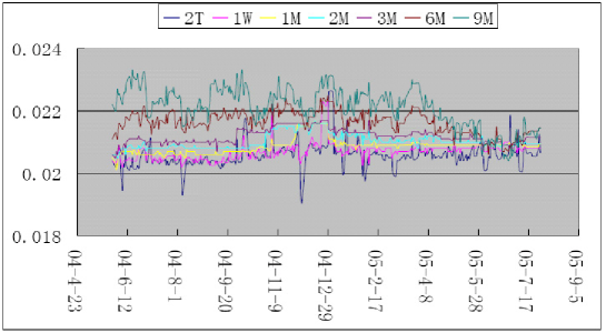
Figure 6.1: Historical deposit rates.

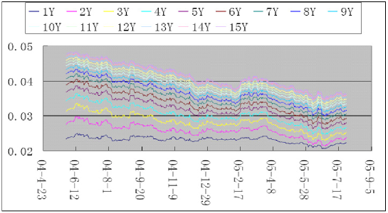
Figure 6.2: Historical spot-starting swap rates.

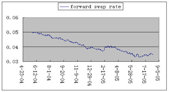
Figure 6.3: Forward swap rates for $T_{1}$.

Swaption Volatility Data

We have access to daily ATM implied volatilities of European swaptions. Each European swaption has two attributes, the expiry and tenor. The expiry can typically take the following 11 values: 1 month, 3 months, 6 months, 1 year, 2 years, 3 years, 4 years, 5 years, 7 years, 10 years and 15 years. The tenor takes one of the 10 values from 1 year to 10 years. Thus every day there are in total 110 ATM quotes available for the European swaptions. From these quotes, we get the ATM volatilities by applying a two-dimensional linear interpolation. For example, Figure 6.4 shows the time series of the ATM volatilities of the European swaption corresponding to underlying co-terminal swap which starts at $T_{2}$. The time series of the corresponding forward swap rates is plotted in the figure as well.

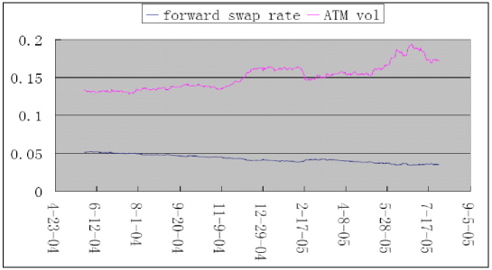
Figure 6.4: ATM volatilities and forward swap rates for $T_{2}$.

Besides we have only access to end-of-month smile quotes for each month of the period. Each European swaption has three attributes, namely, expiry, tenor and strike. Each attribute can take a value in a certain range. Similar to above, we get the required European swaptions’ smile quotes by applying a three-dimensional linear interpolation. Figure 6.5 shows the end-of-month smiles of the European swaption corresponding to the underlying co-terminal swap which starts at $T_{2}$. Each of these smiles are composed of 11 quotes for strikes with the offset to the ATM point varying from -50bp to 50bp. More precisely, there are quotes for strikes with an offset to the ATM level of -50bp, -40bp, -30bp, -20bp, -10bp, 0, 10bp, 20bp, 30bp, 40bp and 50bp.

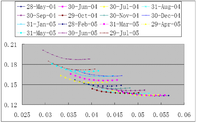
Figure 6.5: End of month smiles for $T_{2}$.

6.2.2 Creating Synthetic Smiles

For a hedging simulation based on a one-day time step, we need daily smile quotes even just for book-keeping of the value of the Bermudan. Thus we need to create smile data for non-end-of-month dates. This is achieved as follows:

• For each end-of-month date, we calibrate the swaptions’ prices to the UVDD model to get the model parameters $\sigma_{n}^{1}$, $\sigma_{n}^{2}$, $\omega_{n}$ and $m_{n}$. In the calibration, we use exactly the same setting corresponding to case 6 in Section 5.2. That is, we have two log-normal components with $\lambda_{n}=0.75$, and $m_{n}$ is restricted within the range $[0,0.10]$;

• For each of the other days, we get the values of $\omega_{n}$ and $m_{n}$ by linear interpolation of the parameters corresponding to the previous and next end-of-month dates. We do the interpolation in terms of these two parameters, because the former is an indicator of the smile shape and the latter of the skew effect. The parameter $\sigma_{n}^{1}$ has been adjusted such that the implied (Black) ATM volatility equals the market quote.

Now we have created the required smile data in terms of the UVDD model parameters for the complete 14 months period on a daily level. Figure 6.6 shows the time series of the UVDD model parameters. In Figure 6.6, the range in which $\omega_{n}$ varies is shown in the y-axis on the right.

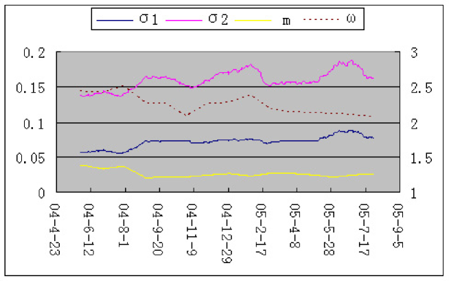
Figure 6.6: UVDD model parameters for $T_{2}$.

6.3 Hedge Test Setup

We set up our hedge test as follows.

1. At the very beginning of the first day, we long a Bermudan swaption by shorting money from our bank account. We keep the Bermudan till the last day of the hedge period. We construct a hedge portfolio containing all the hedging instruments. At the very beginning of the first day, the hedge portfolio contains nothing.

2. Everyday we value the Bermudan and the hedge portfolio. The hedged NPV corresponding to that day is given by

$$\mbox{"hedged NPV"}=\mbox{"Bermudan value"}+\mbox{"hedge portfolio value" + "bank account value"}.$$ (6.1)

3. After that, we add the hedge portfolio’s value to our bank account and liquidate the instruments in the hedge portfolio (constructed in the previous day).

4. Next, we calculate the vega sensitivities of the Bermudan and take positions of European swaptions to neutralize these vega sensitivities. We deduct money from our bank account for setting up these positions (vega hedging).

5. Then, we calculate the delta sensitivities of the Bermudan and the hedge portfolio as a whole. We take positions in spot-starting swaps and deposits to neutralize these delta sensitivities. We again deduct money from our bank account for setting up these positions (delta hedging).

6. Finally, at the end of the day, we add the accrued interest for that day to our bank account.

7. We repeat steps 2. to 6. on a daily basis until the last day of the hedge period.

The above procedure is for a delta+vega hedging simulation. For only a delta hedging simulation, we have to skip the 4th step.

6.4 Sensitivity Calculation

In Pelsser [18], hedging simulations for non-smile Bermudans were conducted. When a vega hedging was set up, ATM European swaptions were used to neutralize the vega sensitivity of the Bermudan. The vega of an ATM European swaption is given by the following formula,

$$\frac{\partial ESN_{n}(t;K)}{\partial\bar{\sigma}}|_{K=S_{n}(t)}=P_{n}(t)S_{n}(t)\phi(d_{+})\sqrt{T_{n}-t},$$ (6.2)

where

$$\begin{cases}\phi(x)=\frac{1}{\sqrt{2\pi}}e^{-\frac{1}{2}x^{2}}\\ d_{+}=\frac{1}{2}\bar{\sigma}\sqrt{T_{n}-t}\\ \mbox{$\bar{\sigma}$ is the Black volatility}\end{cases}.$$

Of course, only ATM European swaptions are used to which the Bermudan shows vega sensitivities. What’s important to mention is, that even for European swaptions, it is assumed that the volatility is flat across all strikes. This means that when we liquidate the European positions on the next day, these are not marked-to-market, but marked-to-model. This was a fairly good approximation when those hedging simulations were performed. Because at that time, the smile effect of the swaption market was much less pronounced than nowadays.

We conduct vega hedging against a smile Bermudan in terms of the UVDD volatilities $\sigma_{n}^{1}$. For example, for our Bermudan trade, we can calculate the sensitivity with respect to $\sigma_{n}^{1},n=1,2,\cdots,10$, i.e., in total 10 vega sensitivities. We can do this by using the following analytical formula,

$$\frac{\partial ESN_{n}(t;K)}{\partial\sigma_{n}^{1}}|_{K=S_{n}(t)}=P_{n}(t)(S_{n}(t)+m_{n})[\lambda_{n}\phi(d_{+}^{1})+(1-\lambda_{n})\phi(d_{+}^{2})\omega_{n}]\sqrt{T_{n}-t},$$ (6.3)

where

$$\begin{cases}\phi(x)=\frac{1}{\sqrt{2\pi}}e^{-\frac{1}{2}x^{2}}\\ d_{+}^{1}=\frac{1}{2}\sigma_{n}^{1}\sqrt{T_{n}-t}\\ d_{+}^{2}=\frac{1}{2}\omega_{n}\sigma_{n}^{1}\sqrt{T_{n}-t}\end{cases}.$$

Then we need to take a certain amount of position for each European to vega hedge against the smile Bermudan. The next day when we liquidate the European positions, we mark the positions to market.

The deposits and spot-starting swaps are the inputs for constructing the yield curve. Thus the changes of the option value with respect to the change of these instruments’ rates are defined as its delta ratios. The way to calculate the delta ratios is the same for both the smile and non-smile cases.

A relevant (payer) spot-starting swap, with the fixed coupon rate at the par level, is used to neutralize the sensitivity to the corresponding spot-starting swap rate. The ratio of the change of the swap value to the change of the par swap rate is

$$\frac{\partial SV(t;K)}{\partial S}|_{K=S} = \frac{\partial[PVBP(S-K)]}{\partial S}|_{K=S}\;\;\;\;\;\;\;\;\;\;\;\;\;\;\;\;\;\;\;\;\mbox{// by Eq. \ref{eq:swap_value}}$$ (6.4)

$$= \{PVBP+(S-K)\frac{\partial PVBP}{\partial S}\}|_{K=S}$$

$$= PVBP,$$

where $S$ denotes the par swap rate.

A relevant deposit is used to neutralize the sensitivity to the corresponding deposit rate. The sensitivity of the value of the deposit to the deposit rate is

$$\frac{\partial("deposit\;value")}{\partial("deposit\;rate")} = \frac{\partial(\frac{1}{1+"deposit\;rate"\times\delta t})}{\partial("deposit\;rate")}$$ (6.5)

$$= -\frac{\delta t}{(1+"deposit\;rate"\times\delta t)^{2}},$$

where $\delta t$ denotes the accrued time associated with the deposit.

Except for the sensitivities described in Equation 6.2, 6.3, 6.4 and 6.5, all the other vega and delta sensitivities are computed numerically by the ”bump and revalue” method. The ”bump and revalue” method is just a simple finite-difference approach to approximate the first derivative,

$$V^{\prime}(x)\approx\frac{V(x+b)-V(x)}{b},$$ (6.6)

where $V(x)$ is the value of an instrument which depends on the underlying factor $x$, and $b$ is the bump size. In our test, the bump size is always set to 1bp, except for the vega of the non-smile Bermudan, which is calculated with a bump size of 10bp. This has been determined by experimenting with different settings. Note that increasing or decreasing the bump size by a factor 10 has little impact for the hedge results.

6.5 Results of Hedge Tests

6.5.1 Comparison between Hedging against Smile Bermudan and the Original Hedging against Non-smile Bermudan

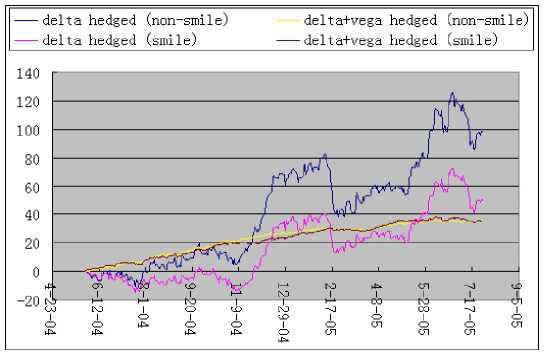
Figure 6.7: Delta and delta+vega hedged NPV (Europeans marked to model in the non-smile case).

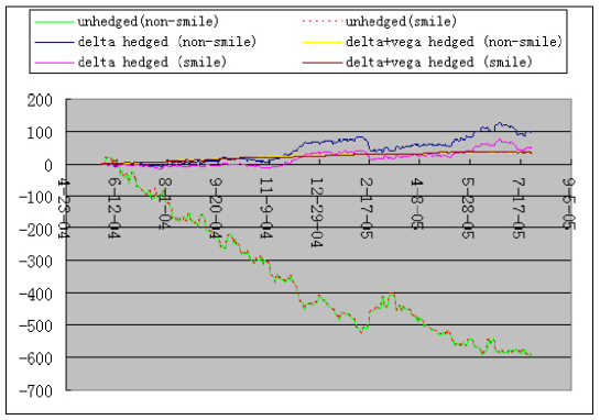
Figure 6.8: Adding the unhedged NPV to Figure 6.7.

For hedging the non-smile Bermudans, we first stick to the approach used in Pelsser [18] as a benchmark. In Figure 6.7, we show the delta and delta+vega hedged NPV for hedging smile and non-smile Bermudans. The mean-reversion parameter is set to zero. The strike of the Bermudan is set to $4.0\%$. This is a near-the-money level, which has the maximal exposure to vega risk. If we check Figure 6.3, the Bermudan is running from a little in-the-money to a little out-of-the-money during the whole hedge period. We see from Figure 6.7 that the smile model has a better delta hedging performance than the non-smile model. But they have similar delta+vega hedging performances. If we put the unhedged NPV along with the hedged NPV, which is shown in Figure 6.8, any of the hedged NPVs has a much smaller order of magnitude.

Monthly Vega-hedging vs Daily Vega-hedging

The transaction cost for trading European swaptions is fairly expensive. In practice, we can not do the vega hedging on a daily basis, but on a monthly basis. Figure 6.9 shows the delta+vega hedged NPV when the European positions are only rolled at the end of each month, together with the original daily delta+vega hedged NPV. We see that in both the smile and non-smile cases, the change from a daily rolling to monthly rolling for vega positions has little impact to the hedged NPV. The vega hedging in all the forth-coming tests is done on a daily basis.

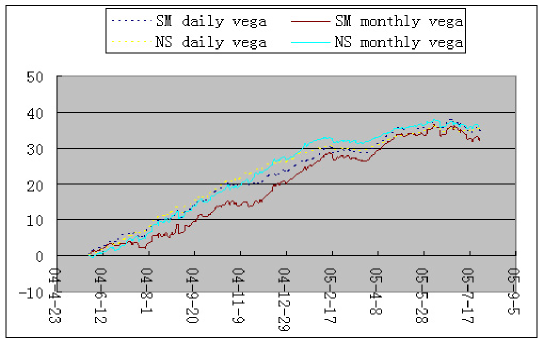
Figure 6.9: Monthly vega-hedging vs daily vega-hedging.

Experiments for Different Settings of the UVDD Model

We have also tested some other settings for the smile vega hedging. These tests are all related to adjustments of the calibration to the end-of-month smile data:

• case 1: When we calibrate the UVDD model, we set the first components’ weight $\lambda_{n}$ to $0.5$ instead of the original $0.75$;

• case 2: When we calibrate the UVDD model, we restrict the displacement coefficient within $(0,0.05)$ instead of the original $(0,0.10)$;

• case 3: We calibrate the UVDD model to only 3 quotes instead of the original 11 quotes. More precisely, there are quotes with relative strikes to the ATM level of -50bp, 0 and 50bp.

We show in Figure 6.10 the delta+vega hedged NPV for each of the three cases described above. The benchmark series is the original delta+vega hedged NPV in the smile case. We see that all these different settings have little impact to the hedged NPV.

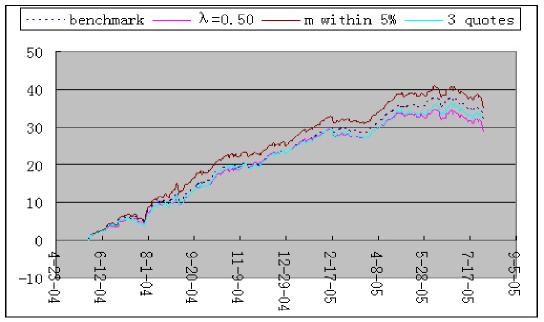
Figure 6.10: Some tunings for the smile vega-hedging.

6.5.2 Marking the Vega-hedging to Market in case of Non-smile Bermudan

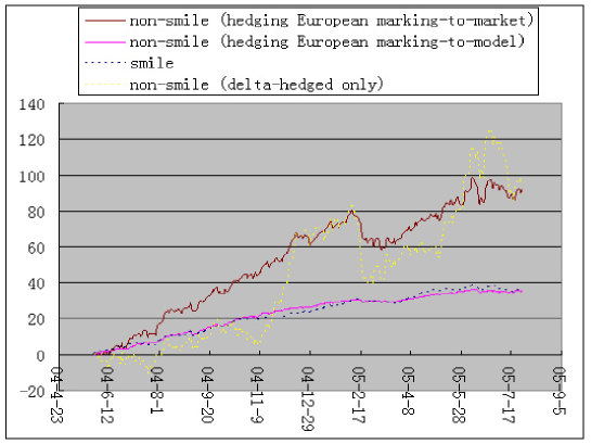
Figure 6.11: Effect of Europeans being marked to model in the non-smile case for its delta+vega hedged NPV.

For the tests described in the previous section, for the non-smile delta+vega hedging simulations, the hedging European swaptions are not marked to market when they are being liquidated. However, for a fair comparison of the hedge performance between the smile and non-smile models, it is consistent to mark European swaptions in the non-smile case to market instead of to the (Black) model. Figure 6.11 shows the new delta+vega hedged NPV in the non-smile case according to the adjustment. For completeness, we have also included in the figure the following data: the original non-smile delta+vega hedged NPV, where the Europeans are marked to model; the smile delta+vega hedged NPV; the non-smile delta hedged NPV.

We see from Figure 6.11 that the marking-to-market version of the non-smile delta+vega hedged NPV has a larger (positive) drift than the marking-to-model one. This can be explained as follows. From Figure 6.2, 6.3 and 6.4, we see that the underlying co-terminal swap rates have an overall decreasing trend. In our hedge test, we long a Bermudan and short ATM (payer) Europeans to kill the vega sensitivities. The next day, the Europeans are most likely to be out of the money because of the decreasing trend of the underlying. We see from Figure 6.5 that the out-of-the-money, but close to ATM, volatility quote is always lower than the ATM quote. This means that on the next day the Europeans marked to market have lower values than those when marked to (Black) model. Because of the short positions, the marking-to-market version’s hedge portfolio has a higher value than the marking-to-model one. This directly leads to a larger drift of the hedged NPV for the former by Equation 6.1. This phenomenon can also be explained in another way. In the original non-smile case, although we take the correct prices for the (ATM) European positions, we are generating the wrong hedge ratios. The next day, if we still mark the Europeans to the wrong model, which generates the wrong ratios, we would get a quite satisfactory hedge result. But if we mark them to market, the hedge performance becomes much worse.

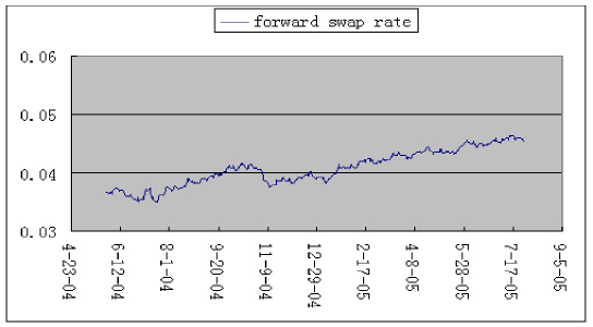
Figure 6.12: Forward swap rates for $T_{1}$ after reversing the historical data.

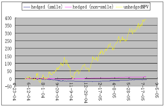
Figure 6.13: Counterpart figure to Figure 6.8 after reversing the historical data.

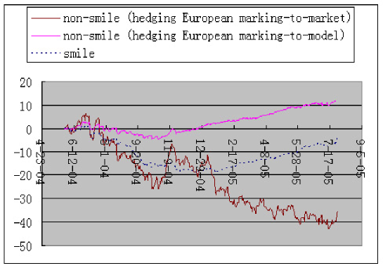
Figure 6.14: Counterpart figure to Figure 6.11 after reversing the historical data.

If we reverse the historical data, we should expect the opposite drift effect in the non-smile case between the marking-to-market and marking-to-model versions. Figure 6.12 shows that the time series of the forward swap rate corresponding to the underlying co-terminal swap which starts at $T_{1}$. Now the underlying has an increasing trend, starting a little out-of-the-money and ending a little in-the-money (strike $4.0\%$). Figure 6.13 is the counterpart figure to Figure 6.8 after reversing the historical data, but without the delta hedged NPV. As expected, we see that the unhedged NPV now has a large positive drift instead of the original very negative one. Figure 6.5 shows that the in-the-money volatility quote is always higher than the ATM quote. This means that on the next day the Europeans marked-to-market have lower values than those when marked to (Black) model. This leads to the opposite effect for the drift. Figure 6.14 is the counterpart figure to Figure 6.11 after reversing the historical data, but without the delta hedged NPV. We see from Figure 6.14 that the marking-to-market version of the non-smile delta+vega hedged NPV has a larger (negative) drift than the marking-to-model one. This is exactly the drift effect we expect for reversing the historical data.

6.5.3 Hedge Tests for ITM/OTM Trades

In Section 6.5.1 and 6.5.2, we only conducted hedge tests for the near-the-money strike ($4.0\%$), which is most sensitive to vega risk. In this section, we perform the counterpart hedging simulations for the in-the-money (ITM) strike ($2.5\%$) and the out-of-the-money (OTM) strike ($5.5\%$).

Let’s first get an impression of the magnitudes of the unhedged NPV. Figure 6.15 shows the unhedged NPV for the ITM/OTM trades, together with the previous near-the-money ones. We see that the ITM unhedged NPV has the largest drift and OTM a fairly small one. The near-the-money unhedged NPV fall in between.

Figure 6.15: Unhedged NPV for the ITM/near-the-money/OTM trades.

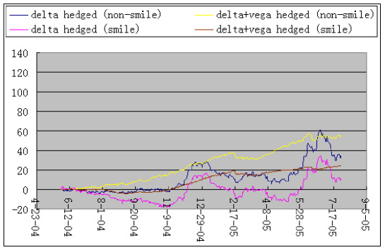
Figure 6.16: Delta and delta+vega hedged NPV for the ITM trade.

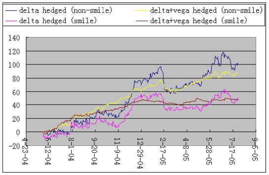
Figure 6.17: Delta and delta+vega hedged NPV for the OTM trade.

In Figure 6.16 and 6.17, we show the delta and delta+vega hedged NPV for hedging smile and non-smile Bermudans with strike levels of $2.5\%$ and $5.5\%$, respectively. Note that in the non-smile cases, the hedging Europeans are marked to market when they are being liquidated. Similar to the results of the near-the-money trade, the smile model outperforms the non-smile model in both delta and delta+vega hedgings.

We also observe that in both smile and non-smile cases, a delta+vega hedging reduces significantly the oscillation of the hedged NPV as compared to the delta hedging. However, it doesn’t affect the drift level of the hedged NPV. This phenomenon can be observed throughout the trades across the three strikes (ITM/near-the-money/OTM). In Figure 6.18, 6.19 and 6.20, we show the standard deviations of the unhedged and hedged daily profit and loss (P$\&$L) for each of the three strikes, respectively. The y-axes in these figures are all in logarithmic scale. The main conclusions are:

• Delta hedging reduces significantly the standard deviation of the unhedged daily P$\&$L. A delta+vega hedging further reduces significantly the standard deviation of the delta hedged daily P$\&$L;

• The smile model outperforms the non-smile model in both the standard deviations of the delta and delta+vega hedged daily P$\&$L.

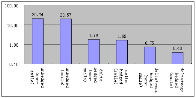
Figure 6.18: Standard deviation of the unhedged and hedged daily P$\&$L ($K=2.5\%$).

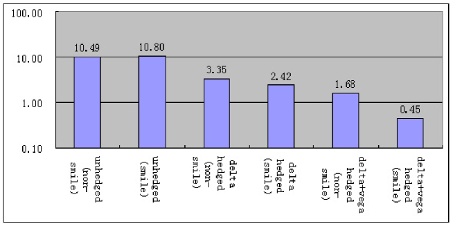
Figure 6.19: Standard deviations of the unhedged and hedged daily P$\&$L ($K=4.0\%$).

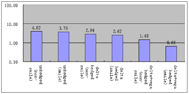
Figure 6.20: Standard deviations of the unhedged and hedged daily P$\&$L ($K=5.5\%$).

6.5.4 Impact of the Mean-reversion Parameter on the Hedge Performance

In all the tests discussed before, the mean-reversion parameter has been set to zero. In this section, we test the impact of the mean-reversion level on the hedge performance. We stick to the delta+vega hedging and a Bermudan with the strike level of $4.0\%$ is considered.

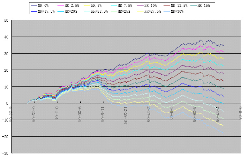
Figure 6.21: Delta+vega hedged NPV in the smile case by setting different values of the mean-reversion (MR) parameter.

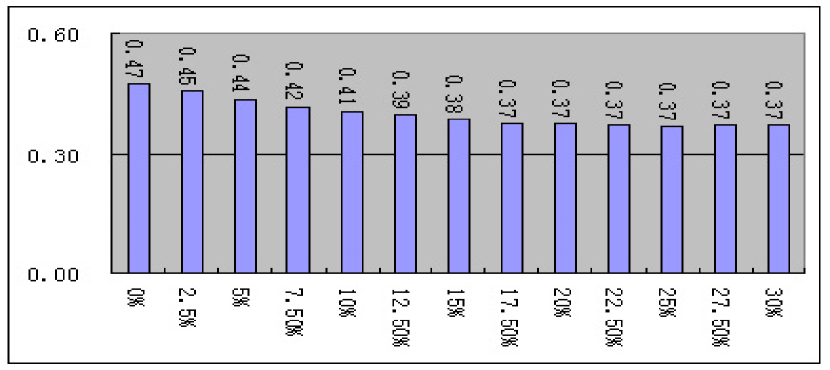
Figure 6.22: Standard deviations of hedged daily P$\&$L corresponding to those tests in Figure 6.21.

In Figure 6.21, we show the hedge results which have been obtained by using different values of the mean-reversion parameter. In Figure 6.22, we show the standard deviations of hedged daily P$\&$L corresponding to those tests in Figure 6.21. From these two figures, we clearly see that increasing the mean-reversion level decreases the level of the hedged NPV’s drift, but has little impact of its oscillation.

By following the approach described in Section 2.3.2, our estimate for the mean-reversion parameter is around $3\%$. Please note this is just a rough estimate. The estimated mean-reversion parameter by that approach is not accurate due to the following two reasons:

• When we choose historical data of different periods, we get different estimated levels;

• Even if we fix a period of historical data, when the Bermudan trade in our hedge test is running towards its first exercise date, the $\rho$ and $\sqrt{\frac{T_{n}}{T_{k}}}$ in Equation 2.37 are both changing over time. This leads to a time-varying mean-reversion level.

We are not in favor of quantifying the mean-reversion level by that approach because of the following reasons:

• The lognormal assumption in Equation 2.32 conflicts the UVDD’s assumption that the terminal density is a mixture of lognormal distributions;

• For determining the marginal density of each individual terminal swap rate, we make use of the current market information (European swaptions). But for determining the joint distribution of the underlying swap rates, we make use of the past information (historical data of swap rates). It is not clear whether these two sources of information are consistent to each other.

• Whether the mean-reversion level is a constant over time is questionable. But even if we used Section 2.3.2’s approach to implement a dynamic mean-reversion estimator, we would introduce another uncertainty, a time-varying or even stochastic MR, which can not be killed by European swaptions in a hedging simulation. One ideal way to solve this problem is to determine the mean-reversion parameter by extracting information from another relevant path-dependent option, which is liquid enough. In this way, we may kill the MR uncertainty in hedging as well as extract consistent market information for the marginal and joint densities of the underlying swap rates.

6.5.5 Discussion of the Residual Drift of the Hedged NPV

Although the smile model achieves a better hedging performance than the non-smile model, there is still a residual drift in the hedged NPV. This might be due to the following reasons:

• A misspecified mean-reversion parameter. This has already been elaborated in Section 6.5.4;

• A mismatch of cash-flows. We are using spot-starting swaps instead of forward swaps for delta-hedging. The payments out of the Bermudan are not exactly offset with the cash-flows out of the spot-starting swaps, but are only offset on an aggregate basis. Pelsser [18] performed an ”exact” hedge, which uses discount bonds to exactly offset the cash-flows from the Bermudan. The test result shows that the ”exact” hedge reduces the drift significantly;

• Other misspecified model parameters. Pelsser [18] explained that even for a European option, a misspecified model parameter may lead to a drift for the delta-hedged NPV, even if the hedging is done continuously. The magnitude of the drift is proportional to the level of gamma. The only way to kill this risk is to gamma hedge the position. Unfortunately, a Bermudan swaption on a multi-dimensional underlying can not be gamma hedged, because we don’t have enough hedging instruments to kill the cross-term sensitivities $\frac{\partial^{2}BSN}{\partial S_{i}\partial S_{j}}$, for $i\neq j$.

Chapter 7 Conclusions $\&$ Suggestions for Future Research

A volatility smile has been successfully incorporated into the Markov-functional model by using the UVDD digital mapping. The new model has a significant impact for pricing Bermudan swaptions, especially for the deep ITM/OTM strikes. The MF model based on the UVDD mapping also improves the hedging performance significantly compared to the MF model based on the Black-Scholes mapping. This is consistent with the fact that the smile model has some freedom to control the implied future smiles and generates fairly good smile dynamics.

However, the method for estimation of the mean-reversion parameter could probably be improved. As discussed in Section 6.5.4, the present approach has some crucial drawbacks. A better approach would be to use relevant path-dependent options which directly contain the information for the joint distribution of the underlying swap rates.

Appendix A Notation and Preliminary Knowledge

A.1 Notation and Preliminary Knowledge

In this appendix, we would like to explain the notation and some preliminary knowledge relevant to this report.

• We choose a tenor structure $T_{1},T_{2},...,T_{N+1}$ where $T_{n}(n=1,2,...,N)$ denotes the n-th floating reset date. In other words, the LIBOR rate $L_{n}$ has a tenor of $[T_{n},T_{n+1}]$ with length $\alpha_{n}=T_{n+1}-T_{n}$; the swap rate $S_{n}$ has a tenor of $[T_{n},T_{N+1}]$ with cash exchange at time $T_{n+1},...,T_{N+1}$.

• Let $D_{n}(t)$ denote the value at time t of a discount bond maturing at $T_{n}$.

• The forward LIBOR rate $L_{n}(t)$ is defined as

  $$L_{n}(t)=\frac{1}{\alpha_{n}}(\frac{D_{n}(t)}{D_{n+1}(t)}-1).$$ (A.1)

• Let $P_{n}(t)$ denote the PVBP, namely present value of a basispoint, on tenor $[T_{n},T_{N+1}]$.

  $$P_{n}(t)=\sum_{k=n+1}^{N+1}\alpha_{k-1}D_{k}(t).$$ (A.2)

  The following linear relationship is of use in MF model’s digital mapping:

  $$\frac{P_{n}(T_{n+1})}{D_{N+1}(T_{n+1})} = \frac{\sum_{k=n+1}^{N+1}\alpha_{k-1}D_{k}(T_{n+1})}{D_{N+1}(T_{n+1})}$$ (A.3)

  $$= \frac{\alpha_{n}+\sum_{k=n+2}^{N+1}\alpha_{k-1}D_{k}(T_{n+1})}{D_{N+1}(T_{n+1})}$$

  $$= \frac{\alpha_{n}+P_{n+1}(T_{n+1})}{D_{N+1}(T_{n+1})}=\frac{\alpha_{n}}{D_{N+1}(T_{n+1})}+\frac{P_{n+1}(T_{n+1})}{D_{N+1}(T_{n+1})}.$$

• A payer swap pays the fixed leg and receives the floating leg; a receiver swap receives the fixed leg and pays the floating leg.

• The forward par swap rate $S_{n}(t)$ on tenor $[T_{n},T_{N+1}]$ can be expressed as

  $$S_{n}(t)=\frac{D_{n}(t)-D_{N+1}(t)}{P_{n}(t)}.$$ (A.4)

• Denote the forward measure for the numeraire $P_{n}(t)$ by $Q^{n,N+1}$. Then the forward swap rate $S_{n}(t)$ is a $Q^{n,N+1}$-martingale.

• Let $SV_{n}(t;K)$ denote the value at time t of a swap with a fixed rate K on tenor $[T_{n},T_{N+1}]$ with unit notional amount. The value of the swap is

  $$SV_{n}(t;K)=P_{n}(t)\varphi(S_{n}(t)-K),$$ (A.5)

  where $\varphi$ is 1 for a payer swap and -1 for a receiver swap.

• Let $SV(t;K)$ denote the value at time t of the swap with a fixed rate K on tenor $[T_{n},T_{N+1}]$ with unit notional amount where $T_{n-1}<t\leq T_{n}$. In other words, $SV(t;K)$ denotes the value of the swap that has the closet starting date among all the co-terminal swaps with the same fixed rate K.

• Let $DSN_{n}(t;K)$ denote the value at time t of a Digital swaption expiring at time $T_{n}$ with strike K on a swap on tenor $[T_{n},T_{N+1}]$ with unit notional amount. A Digital swaption pays the amount of $P_{n}(T_{n})$ if it expires in the money and nothing otherwise. It can be expressed under the forward measure $Q^{n,N+1}$ by using the martingale property,

  $$DSN_{n}(t;K) = P_{n}(t)\mathbb{E}_{t}^{n,N+1}[\frac{DSN_{n}(T_{n};K)}{P_{n}(T_{n})}]$$ (A.6)

  $$= P_{n}(t)\mathbb{E}_{t}^{n,N+1}[\frac{P_{n}(T_{n})I_{\{\varphi(S_{n}(T_{n})-K)>0\}}}{P_{n}(T_{n})}]$$

  $$= P_{n}(0)\mathbb{E}_{t}^{n,N+1}[I_{\{\varphi(S_{n}(T_{n})-K)>0\}}]$$

  $$= P_{n}(t)\int_{-\infty}^{\infty}I_{\{\varphi(y-K)>0\}}\phi(y)dy,$$

  where $\phi$ denotes the probability density function under $Q^{n,N+1}$ of the terminal swap rate $S_{n}(T_{n})$ and $\varphi$ is 1 for a payer Digital swaption and -1 for a receiver one. Assuming a lognormal distribution, we derive the Black formula of a Digital swaption by some algebra

  $$DSN_{n}(t;K)=P_{n}(t)\Phi(\varphi\frac{\log(S_{n}(t)/K)-\frac{1}{2}\bar{\sigma}_{n}^{2}(T_{n}-t)}{\bar{\sigma}_{n}\sqrt{T_{n}-t}}),$$ (A.7)

  where $\bar{\sigma}_{n}$ is the swaption’s implied volatility.

• Let $ESN_{n}(t;K)$ denote the value at time t of a European swaption expiring at time $T_{n}$ with strike K on a swap with tenor $[T_{n},T_{N+1}]$ and unit notional amount. It can be expressed under the forward measure $Q^{n,N+1}$ by the martingale property,

  $$ESN_{n}(t;K) = P_{n}(t)\mathbb{E}_{t}^{n,N+1}[\frac{ESN_{n}(T_{n};K)}{P_{n}(T_{n})}]$$ (A.8)

  $$= P_{n}(t)\mathbb{E}_{t}^{n,N+1}[\frac{SV_{n}(t;K)I_{\{\varphi(S_{n}(T_{n})-K)>0\}}}{P_{n}(T_{n})}]$$

  $$= P_{n}(t)\mathbb{E}_{t}^{n,N+1}[\frac{P_{n}(T_{n})\varphi(S_{n}(T_{n})-K)I_{\{\varphi(S_{n}(T_{n})-K)>0\}}}{P_{n}(T_{n})}]$$

  $$= P_{n}(t)\mathbb{E}_{t}^{n,N+1}[\varphi(S_{n}(T_{n})-K)I_{\{\varphi(S_{n}(T_{n})-K)>0\}}]$$

  $$= P_{n}(t)\int_{-\infty}^{\infty}\varphi(y-K)I_{\{\varphi(y-K)>0\}}\phi(y)dy,$$

  where $\phi$ denotes the probability density function of $S_{n}(T_{n})$, and $\varphi$ is 1 for a payer European swaption and -1 for a receiver one. Assuming a lognormal distribution, we have the Black formula for a European swaption

  $$ESN_{n}(t;K)=\varphi P_{n}(t)(S_{n}(t)\Phi(\varphi d_{+})-K\Phi(\varphi d_{-})),$$ (A.9)

  where

  $$d_{\pm}=\frac{\log(\frac{S_{n}(t)}{K})\pm\frac{1}{2}\bar{\sigma}_{n}^{2}(T_{n}-t)}{\bar{\sigma}_{n}\sqrt{T_{n}-t}}.$$

  It should be noted that by differentiating Equation A.8 with respect to strike $K$, we get the Digital swaption’s value in Equation A.6, i.e.,

  $$DSN_{n}(t;K)=-\varphi\frac{\partial ESN_{n}(t;K)}{\partial K}.$$ (A.10)

  It’s important to realize that we can only observe the implied volatility quotes of European swaptions in the market. The values of Digital swaptions are uniquely implied from their European counterparts by the no-arbitrage principle, which is model-independent.
  
  If we further differentiate Equation A.6 with respect to $K$, we get the underlying’s probability density function under $Q^{n,N+1}$, i.e.,

  $$\phi(K)=\frac{\partial DSN_{n}(t;K)}{\partial K}.$$ (A.11)

  A useful idea is that rather than from the European options, we may equivalently imply the underlying’s density from their Digital counterparts, which is one step less complicated.

• Let $BSN(t;K)$ denote the value at time t of a co-terminal Bermudan swaption with strike K on a swap with a unit notional amount. A co-terminal Bermudan entitles the swaption holder to enter on several predetermined dates into a swap that ends at a fixed maturity date.

A.2 Simplification of Notation

As we are interested only in the discrete time points of tenor structure $T_{1},T_{2},...,T_{N+1}$, we apply some simplification to make our math expressions more compact. We first simplify $X(T_{n})$ as follows.

$$X_{n}\triangleq X(T_{n}),$$ (A.12)

where n=1, 2, …, N+1. We denote a certain value of $X_{n}$ by $x_{n}$. Moreover we omit the time parameter for a state variable, for example,

$$D_{k}(X_{n})\triangleq D_{k}(T_{n},X_{n})=D_{k}(T_{n},X(T_{n})),$$ (A.13)

or for a sample point

$$D_{k}(x_{n})\triangleq D_{k}(T_{n},x_{n}),$$ (A.14)

where $k\geq n$, since time is always a parameter of a state variable by default. Likewise, we have

$$L_{n}(X_{n}) \triangleq L_{n}(T_{n},X(T_{n}))$$

$$P_{n}(X_{n}) \triangleq P_{n}(T_{n},X(T_{n}))$$

$$S_{n}(X_{n}) \triangleq S_{n}(T_{n},X(T_{n}))$$ (A.15)

$$SV_{n}(X_{n};K) \triangleq SV_{n}(T_{n},X(T_{n});K)$$

$$SV(X_{n};K) \triangleq SV(T_{n},X(T_{n});K)$$

$$DSN_{n}(X_{n};K) \triangleq DSN_{n}(T_{n},X(T_{n});K)$$

$$ESN_{n}(X_{n};K) \triangleq ESN_{n}(T_{n},X(T_{n});K)$$

$$BSN(X_{n};K) \triangleq BSN(T_{n},X(T_{n});K).$$

A.3 The Greeks

If $V(t,S_{t})$ is the value of a derivative, where $S_{t}$ denotes the value of the underlying, the definition of some sensitivity ratios of $V(t,S_{t})$ are listed below. They are denoted by Greek letters (except Vega) by convention.

$$\mbox{Delta}: \Delta\triangleq \frac{\partial V(t,s)}{\partial s}$$ (A.16)

$$\mbox{Gamma}: \Gamma\triangleq \frac{\partial^{2}V(t,s)}{\partial s^{2}}$$ (A.17)

$$\mbox{Theta}: \Theta\triangleq \frac{\partial V(t,S_{t})}{\partial t}$$ (A.18)

$$\mbox{Vega}: \mathcal{V}\triangleq \frac{\partial V(t,S_{t})}{\partial\sigma}.$$ (A.19)

For Vega’s definition in Equation A.19, $\sigma$ denotes the volatility of the underlying.

Appendix B Integration of Polynomials against Gaussians

This appendix closely follows Pelsser [17][19]. The numerical integration discussed here is based on the following idea:
1. fit a polynomial to the payoff function defined on the grid;
2. calculate analytically the integral of the polynomial against the Gaussian distribution.

Fitting a Polynomial. Given a number of points $x_{i}$ and a set of function values $f_{i}$, a polynomial that fits through these values can be computed recursively using Neville’s algorithm. Let $P_{(i)\ldots(i+m)}$ denote the polynomial defined using the points $x_{i},\ldots,x_{i+m}$. Then the following relationship holds

$$P_{(i)\ldots(i+m)}=\begin{cases}\frac{(x-x_{i+m})P_{(i)\ldots(i+m-1)}+(x_{i}-x)P_{(i+1)\ldots(i+m)}}{x_{i}-x_{i+m}}&\mbox{if $m\geq 1$}\\ \;\;\;\;\;f_{i}&\mbox{if $m=0$}\end{cases}$$ (B.1)

where $m$ is the order for polynomial fitting. Each polynomial can be expressed as $P_{(i)\ldots(i+m)}=\sum_{k=0}^{m}c_{i,k}x^{k}$. Using Equation B.1 we can then derive a recurrence formula for the coefficients $c_{i,k}$ as follows

$$c_{i,m} = \frac{c_{i,m-1}-c_{i+1,m-1}}{x_{i}-x_{i+m}}$$

$$c_{i,k} = \frac{x_{i}c_{i+1,k}-x_{i+m}c_{i,k}+c_{i,k-1}-c_{i+1,k-1}}{x_{i}-x_{i+m}}\;\;\;\;\;\;\;1\leq k\leq m-1$$ (B.2)

$$c_{i,0} = \frac{x_{i}c_{i+1,0}-x_{i+m}c_{i,0}}{x_{i}-x_{i+m}}$$

Integrating against Gaussian. The Markov process $x$ defined in Equation 2.13 has Gaussian density functions. Hence, the calculation of integrals against a Gaussian density can be reduced to evaluating for different powers $x^{k}$ of the polynomial $P$ the following integral

$$G(k;h,\mu,\sigma)=\int_{-\infty}^{h}x^{k}\frac{exp\{-\frac{1}{2}(\frac{x-\mu}{\sigma})^{2}\}}{\sigma\sqrt{2\pi}}dx$$ (B.3)

Using partial integration, we derive the following recurrence relation for $G$ in terms of $k$

$$G(k) = \mu G(k-1)+(k-1)\sigma^{2}G(k-2)-\sigma^{2}h^{k-1}\frac{exp\{-\frac{1}{2}(\frac{x-\mu}{\sigma})^{2}\}}{\sigma\sqrt{2\pi}}\;\;\;k\geq 1$$ (B.4)

$$G(0) = N(\frac{h-\mu}{\sigma})\;\;\;\;\mbox{and}\;\;\;\;G(-1)\;\;=\;\;0$$

where $N(.)$ denotes the standard normal distribution function.

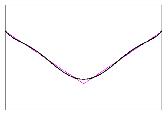
Figure B.1: Bad polynomial fit

Calculating Expected Values. Given a grid on which we are working, option values are calculated by taking expectations of the value function against the Gaussian density. Given that we have calculated several option values at time $T_{n+1}$ at grid points $x_{j}$, we want to calculate option vales at time $T_{n}$ for grid points $x_{i}$. To do this we proceed as follows.

• Given an order $M$ the approximating polynomial $P(j-M/2)\ldots(j+1+M/2)$ for the interval $[x_{j},x_{j+1}]$ is fitted through the points $x_{j-M/2},\ldots,x_{j+1+M/2}$, where $M/2$ denotes integer division ($M$ div 2). The approximating polynomial has coefficients $c_{j,k}$.

• The integral over the approximating polynomial for the interval $[x_{j},x_{j+1}]$ can now be expressed as

  $$\sum_{k=0}^{M}c_{j,k}\{\;G(\;k;x_{j+1},x_{i},\sqrt{Var(X(T_{n+1})|X(T_{n})=x_{i})}\;)$$

  $$-\;G(\;k;x_{j},x_{i},\sqrt{Var(X(T_{n+1})|X(T_{n})=x_{i})}\;)\;\}$$ (B.5)

  where $Var(X(T_{n+1})|X(T_{n})=x_{i})=\int_{T_{n}}^{T_{n+1}}\tau^{2}(u)du$.

• The option value in grid point $x_{i}$ will now be given by summing over all intervals $[x_{j},x_{j+1}]$:

  $$\sum_{j}\sum_{k=0}^{M}c_{j,k}\{\;G(\;k;x_{j+1},x_{i},\sqrt{Var(X(T_{n+1})|X(T_{n})=x_{i})}\;)$$

  $$-\;G(\;k;x_{j},x_{i},\sqrt{Var(X(T_{n+1})|X(T_{n})=x_{i})}\;)\;\}$$ (B.6)

• Loop over all points $x_{i}$.

The fitting of the polynomials works well if the function that one wants to approximate is smooth. However, many option payoffs are determined as the maximum of two functions. This implies that the payoff function will be smooth except at the crossover point where the payoff function may have a kink. Since polynomials are ”stiff” they will fit a function with a kink very poorly. This is shown in Figure B.1. The way this problem can be solved is to fit polynomials to both underlying functions, and to split the integration interval at the crossover point, using the appropriate polynomial on either side of the crossover point.

Appendix C Some Derivations

C.1 Derivation of Equation 2.15 in Section 2.2.1

By Equation 2.13 and setting $X_{0}=0$, we have

$$X(s) = \int_{0}^{s}\tau(u)dW^{N+1}_{u}$$ (C.1)

$$= \int_{0}^{t}\tau(u)dW^{N+1}_{u}+\int_{t}^{s}\tau(u)dW^{N+1}_{u}$$

$$= X(t)+\int_{t}^{s}\tau(u)dW^{N+1}_{u},$$

$\tau(u)$ is a deterministic function, so $\int_{t}^{s}\tau(u)dW^{N+1}_{u}$ is normally distributed. This results in that conditional on $X(t)=x_{t}$, $X(s)$ is normally distributed with mean equal to

$$\mathbb{E}(X(s)|X(t)=x_{t}) = \mathbb{E}(X(t)+\int_{t}^{s}\tau(u)dW^{N+1}_{u}|X(t)=x_{t})$$ (C.2)

$$= x_{t}+\mathbb{E}(\int_{t}^{s}\tau(u)dW^{N+1}_{u}|X(t)=x_{t})$$

$$= x_{t}+0=x_{t},$$

and variance equal to

$$Var(X(s)|X(t)=x_{t}) = Var(X_{t}+\int_{t}^{s}\tau(u)dW^{N+1}_{u}|X(t)=x_{t})$$ (C.3)

$$= 0+Var(\int_{t}^{s}\tau(u)dW^{N+1}_{u}|X(t)=x_{t})$$

$$= \mathbb{E}[(\int_{t}^{s}\tau(u)dW^{N+1}_{u})^{2}|X(t)=x_{t}]-[\mathbb{E}(\int_{t}^{s}\tau(u)dW^{N+1}_{u}|X(t)=x_{t})]^{2}$$

$$= \mathbb{E}[\int_{t}^{s}\tau^{2}(u)du|X(t)=x_{t}]-0^{2}$$

$$= \int_{t}^{s}\tau^{2}(u)du.$$

Thus the probability density function of $X(s)$ given $X(t)=x_{t}$ is

$$\phi(X(s)|X(t)=x_{t})=\frac{exp(-\frac{1}{2}\frac{(X(s)-x_{t})^{2}}{\int_{t}^{s}\tau^{2}(u)du})}{\sqrt{2\pi\int_{t}^{s}\tau^{2}(u)du}}.$$ (C.4)

Besides, the Markov process $X(t)$ in this choice is time-inhomogeneous as

$$\phi[X(s)|X(t)=x] = \frac{exp(-\frac{1}{2}\frac{(X(s)-x)^{2}}{\int_{t}^{s}\tau^{2}(u)du})}{\sqrt{2\pi\int_{t}^{s}\tau^{2}(u)du}}$$ (C.5)

$$\neq \phi[X(s-t)|X_{0}=x]=\frac{exp(-\frac{1}{2}\frac{(X(s-t)-x)^{2}}{\int_{0}^{s-t}\tau^{2}(u)du})}{\sqrt{2\pi\int_{0}^{s-t}\tau^{2}(u)du}}.$$

C.2 Derivation of Equation 2.29 and 2.31 in Section 2.3.1

Derivation of Equation 2.29 in Section 2.3.1

Multiplying both sides of Equation 2.28 by $e^{at}$ and re-arranging it, we can get

$$e^{at}\theta(t)dt+e^{at}\sigma dW_{t}=e^{at}dr_{t}+ae^{at}r_{t}dt=d(e^{at}r_{t}).$$ (C.6)

Integrating both sides from $0$ to $t$, we have

$$e^{at}r_{t}-r_{0}=\int_{0}^{t}e^{au}\theta(u)du+\sigma\int_{0}^{t}e^{au}dW_{u},$$ (C.7)

that is,

$$r_{t}=e^{-at}r_{0}+e^{-at}\int_{0}^{t}e^{au}\theta(u)du+e^{-at}\sigma\int_{0}^{t}e^{au}dW_{u}.$$ (C.8)

Thus we have, for $t<s$,

$$Corr(r(t),r(s)) = \frac{Cov(r(t),r(s))}{\sqrt{Var(r(t))Var(r(s))}}$$ (C.9)

$$= \frac{E[(e^{-at}\sigma\int_{0}^{t}e^{au}dW_{u})(e^{-as}\sigma\int_{0}^{s}e^{au}dW_{u})]}{\sqrt{E[(e^{-at}\sigma\int_{0}^{t}e^{au}dW_{u})^{2}]E[(e^{-as}\sigma\int_{0}^{s}e^{au}dW_{u})^{2}]}}$$

$$= \sqrt{\frac{E[(\int_{0}^{t}e^{au}dW_{u})^{2}]}{E[(\int_{0}^{s}e^{au}dW_{u})^{2}]}}$$

$$= \sqrt{\frac{\int_{0}^{t}(e^{au})^{2}du}{\int_{0}^{s}(e^{au})^{2}du}}$$

$$= \begin{cases}\sqrt{\frac{t}{s}}&\mbox{if $a=0$}\\ \sqrt{\frac{e^{2at}-1}{e^{2as}-1}}&\mbox{if $a\neq 0$}\end{cases}.$$

Derivation of Equation 2.31 in Section 2.3.1

By Equation C.1 and 2.30, we have, for $t<s$,

$$Corr(X(t),X(s)) = \frac{Cov(X(t),X(s))}{\sqrt{Var(X(t))Var(X(s))}}$$ (C.10)

$$= \frac{Cov(\int_{0}^{t}e^{au}dW_{u},\int_{0}^{s}e^{au}dW_{u})}{\sqrt{Var(\int_{0}^{t}e^{au}dW_{u})Var(\int_{0}^{s}e^{au}dW_{u})}}$$

$$= \frac{E[\int_{0}^{t}e^{au}dW_{u}\int_{0}^{t}e^{au}dW_{u}]}{\sqrt{E[(\int_{0}^{t}e^{au}dW_{u})^{2}]E[(\int_{0}^{s}e^{au}dW_{u})^{2}]}}$$

$$= \sqrt{\frac{E[(\int_{0}^{t}e^{au}dW_{u})^{2}]}{E[(\int_{0}^{s}e^{au}dW_{u})^{2}]}}$$

$$= \sqrt{\frac{\int_{0}^{t}(e^{au})^{2}du}{\int_{0}^{s}(e^{au})^{2}du}}$$

$$= \begin{cases}\sqrt{\frac{t}{s}}&\mbox{if $a=0$}\\ \sqrt{\frac{e^{2at}-1}{e^{2as}-1}}&\mbox{if $a\neq 0$}\end{cases}.$$

Appendix D Near-the-money Bermudan Swaption Prices Affected by More Pronounced Smiles

This appendix gives an explanation of the issue discussed in Section 3.2.4 by considering an example. More precisely, more pronounced smiles, i.e., distributions of the underlying swap rates with fatter tails (both left side and right side), may result in either a higher or lower near-the-money Bermudan value. Recall Equation 2.16 and that by assuming $\alpha_{k}=1$, for $k=n,\cdots,N$, we have

$$S_{n}(X_{n}) = \frac{1-D_{N+1}(X_{n})}{\sum_{k=n+1}^{N+1}D_{k}(X_{n})}$$ (D.1)

$$= \frac{1-D_{N+1}(X_{n})}{D_{n+1}(X_{n})+\sum_{k=n+2}^{N+1}D_{k}(X_{n})}$$

$$= \frac{1-D_{N+1}(X_{n})}{\frac{1}{1+L_{n}(X_{n})}+\sum_{k=n+2}^{N+1}D_{k}(X_{n})}.$$

Rearranging it we have

$$L_{n}(X_{n})=\frac{1}{\frac{1-D_{n+1}(X_{n})}{S_{n}(X_{n})}-{\sum_{k=n+2}^{N+1}D_{k}(X_{n})}}-1.$$ (D.2)

By observation of Equation D.2 we claim that in MF, distributions of swap rates $S_{n}(X_{n})$ with fatter tails may result in fatter-tailed distributions of LIBOR rates $L_{n}(X_{n})$, for $n=1,\cdots,N$.

An evidence of this claim is shown in Figure D.1 and D.2. In Figure D.1, we plot $L_{10}(X_{10})$ in case 5 and 6 mentioned in Section 3.2.4, respectively, together with the probability distribution function of $X_{10}$. Smiles in case 6 are more pronounced than in case 5. We see from the figure that the distribution of $L_{10}(X_{10})$ in case 6 has fatter tails than in case 5. If we plot the similar graphs with respect to $L_{n}(X_{n})$, for $n=1,\cdots,9$, we would reach the same conclusion. Figure D.2 is with respect to case 7 and 8 mentioned in Section 3.2.4, where we can reach exactly the same conclusions as above.

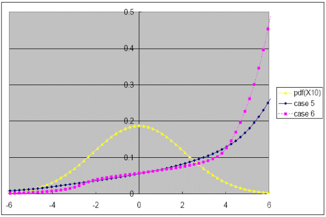
Figure D.1: $L_{10}(X_{10})$ in case 5 and 6.

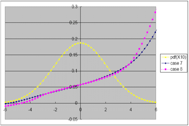
Figure D.2: $L_{10}(X_{10})$ in case 7 and 8.

Based on the validity of the claim above, we make one extremely simplified example. In this example, there are only two floating reset dates $T_{1}$ and $T_{2}$. Each tenor’s length $\alpha_{n}$, for $n=1,2$, is one year. $T_{1}$ is one year ahead of ”now”, i.e., $T_{0}$. At each $T_{n}$, for $n=1,2$, there are only three states, shown in Table D.1. These three states represent the deep ITM, near-the-money and deep OTM scenarios, respectively. The transition probabilities are assigned below:

$$\mathbb{P}(x0\rightarrow x_{1,j}) = \frac{1}{3},\;\;\;\mbox{for $j=-1,0,1$}$$

$$\mathbb{P}(x_{1,i}\rightarrow x_{2,j}) = \frac{1}{3},\;\;\;\mbox{for $i,j=-1,0,1$}.$$

$T_{0}$	$T_{1}$	$T_{2}$
	$x_{1,1}$	$x_{2,1}$
$x_{0}$	$x_{1,0}$	$x_{2,0}$
	$x_{1,-1}$	$x_{2,-1}$

Table D.1: Example - lattice of $X_{n}$.

The corresponding LIBOR tree is shown in Table D.2. We are dealing with a payer Bermudan with the right to exercise at $T_{1}$ and $T_{2}$. The notional is 10000. The swap value tree is computed in Table D.3. In Table D.4, we follow the principle in Section 2.4 to calculate the Bermudan value with the strike level $5.50\%$, which is near the money. The Bermudan price is 122.49. With similar calculations, We also get the Bermudan prices of 250.43 and 44.93 for the strike level $4.50\%$ (ITM) and $6.50\%$ (OTM), respectively.

$T_{0}$	$T_{1}$	$T_{2}$
	$L_{1}(x_{1,1})=7.00\%$	$L_{2}(x_{2,1})=8.00\%$
$L_{0}(x_{0})=5.50\%$	$L_{1}(x_{1,0})=5.50\%$	$L_{2}(x_{2,0})=6.00\%$
	$L_{1}(x_{1,-1})=4.00\%$	$L_{2}(x_{2,-1})=4.00\%$

Table D.2: Example - LIBOR tree.

$SV(x_{1,1})$ =	$SV(x_{2,1})$ =
$10000\times(7.00\%-5.50\%)+\frac{(250+50-150)}{3\times(1+7.00\%)}$	$10000\times(8.00\%-5.50\%)$
= 196.73	= 250.00
$SV(x_{1,0})$=	$SV(x_{2,0})$ =
$10000\times(5.50\%-5.50\%)+\frac{(250+50-150)}{3\times(1+5.50\%)}$	$10000\times(6.00\%-5.50\%)$
=47.39	= 50.00
$SV(x_{1,-1})$=	$SV(x_{2,-1})$=
$10000\times(4.00\%-5.50\%)+\frac{(250+50-150)}{3\times(1+4.00\%)}$	$10000\times(4.00\%-5.50\%)$
= -101.92	= -150.00

Table D.3: Example - payer swap value tree for $K=5.50\%$.

	$BSN(x_{1,1})$=	$BSN(x_{2,1})$=
	$Max(196.73,\frac{(250+50-150)}{3\times(1+7.00\%)})$	Max(250.00,0)
	= 196.73	= 250.00
$BSN(x_{0})$=	$BSN(x_{1,0})$=	$BSN(x_{2,0})$=
$\frac{(196.73+94.79-96.15)}{3\times(1+5.50\%)}$	$Max(47.39,\frac{(250+50-150)}{3\times(1+5.50\%)})$	Max(50.00,0)
= 122.49	= 94.79	= 50.00
	$BSN(x_{1,-1})$=	$BSN(x_{2,-1})$=
	$Max(-101.92,\frac{(250+50-150)}{3\times(1+4.00\%)})$	Max(-150.00,0)
	= 96.15	= -150.00

Table D.4: Example - payer Bermudan swaption value tree for $K=5.50\%$.

Now we have in Table D.5 a LIBOR tree with fatter tails than the original one in Table D.2. Following a similar line above, we get the Bermudan prices of 252.52, 125.08 and 46.43 for the strike level $4.50\%$ (ITM), $5.50\%$ (near-the-money) and $6.50\%$ (OTM), respectively. In this case, more pronounced smiles result in a higher near-the-money Bermudan price.

$T_{0}$	$T_{1}$	$T_{2}$
	$L_{1}(x_{1,1})=7.05\%$	$L_{2}(x_{2,1})=8.05\%$
$L_{0}(x_{0})=5.50\%$	$L_{1}(x_{1,0})=5.50\%$	$L_{2}(x_{2,0})=6.00\%$
	$L_{1}(x_{1,-1})=3.95\%$	$L_{2}(x_{2,-1})=3.95\%$

Table D.5: Example - LIBOR tree of fatter-tailed distribution (A).

However we have in Table D.6 another LIBOR tree which also has fatter tails than the original one. We instead get the Bermudan prices of 252.65, 122.06 and 46.41 for the strike level $4.50\%$ (ITM), $5.50\%$ (near-the-money) and $6.50\%$ (OTM), respectively. In this case, more pronounced smiles result in a lower near-the-money Bermudan price.

$T_{0}$	$T_{1}$	$T_{2}$
	$L_{1}(x_{1,1})=7.05\%$	$L_{2}(x_{2,1})=8.05\%$
$L_{0}(x_{0})=5.50\%$	$L_{1}(x_{1,0})=5.60\%$	$L_{2}(x_{2,0})=5.90\%$
	$L_{1}(x_{1,-1})=3.95\%$	$L_{2}(x_{2,-1})=3.95\%$

Table D.6: Example - LIBOR tree of fatter-tailed distribution (B).

From this example, we see that whether more pronounced smiles result in a higher or lower near-the-money Bermudan price may be subject to how the near-the-money LIBOR probability mass is influenced.

Appendix E Market Data and Specification of Test Trades

E.1 Market Data Used in the Numerical Tests

All the data sets in this report are chosen arbitrarily.

E.1.1 Data Set I

The yield curve in this data set is listed in Table E.1. For example, the fifth row of the table represents the bid/ask discount factor of 367 days from today (July 9th, 2002). Any required discount factor not available in the table was calculated by linear interpolation.

Days	Bid / Ask
34	0.998367115 / 0.998367115
94	0.995269154 / 0.995269154
188	0.990025493 / 0.990025493
367	0.977629093 / 0.977629093
735	0.938822503 / 0.938822503
1098	0.893023545 / 0.893023545
1463	0.84517874 / 0.84517874
1828	0.796865431 / 0.796865431
2562	0.703583273 / 0.703583273
3655	0.5784443 / 0.5784443
5481	0.40916987 / 0.40916987
10961	0.152839928 / 0.152839928

Table E.1: Yield curve of July 9th, 2002.

The implied volatility surface (tenor length, expiry) of ATM European swaptions in this data set is listed in Table E.2. The value of each volatility is the average of the original bid and ask values. Any required volatility not available in the table was calculated by linear surface interpolation.

	Exp. (Days)
Tenor (Days)	32	63	92	182	360	730	1095	1463	1827
360	0.457	0.4455	0.434	0.379	0.333	0.261	0.239	0.219	0.204
720	0.39	0.3805	0.371	0.338	0.294	0.25	0.23	0.213	0.2
1080	0.32	0.32	0.32	0.301	0.271	0.237	0.22	0.206	0.193
1440	0.29	0.29	0.29	0.279	0.255	0.228	0.213	0.2	0.188
1800	0.271	0.2705	0.27	0.263	0.244	0.221	0.208	0.195	0.184
2520	0.25	0.2475	0.245	0.242	0.228	0.211	0.2	0.188	0.177
3600	0.23	0.2265	0.223	0.223	0.213	0.201	0.19	0.178	0.168
5400	0.19	0.1905	0.191	0.191	0.185	0.179	0.17	0.161	0.152
10800	0.19	0.173	0.156	0.155	0.152	0.152	0.143	0.136	0.129

Table E.2: ATM volatility surface of July 9th, 2002.

E.1.2 Data Set II

In this data set, the yield curve of EURO is listed in Table E.3. Any required discount factor not available in the table was calculated by linear interpolation.

Days	Bid / Ask	Days	Bid / Ask
4	0.999658 / 0.999658	1466	0.855901 / 0.855901
11	0.999057 / 0.999057	1830	0.821377 / 0.821377
35	0.996992 / 0.996992	2196	0.787538 / 0.787538
40	0.996575 / 0.996575	2561	0.754289 / 0.754289
66	0.994276 / 0.994276	2926	0.721887 / 0.721887
96	0.991506 / 0.991506	3293	0.690247 / 0.690247
131	0.988237 / 0.988237	3657	0.659733 / 0.659733
221	0.97932 / 0.97932	4022	0.62999 / 0.62999
222	0.979217 / 0.979217	4387	0.601379 / 0.601379
313	0.969993 / 0.969993	4752	0.573949 / 0.573949
314	0.969891 / 0.969891	5120	0.547413 / 0.547413
404	0.960723 / 0.960723	5484	0.522205 / 0.522205
405	0.960621 / 0.960621	7311	0.412457 / 0.412457
495	0.951481 / 0.951481	9135	0.327908 / 0.327908
586	0.942281 / 0.942281	10962	0.262923 / 0.262923
677	0.933159 / 0.933159	14614	0.171647 / 0.171647
678	0.933059 / 0.933059	18267	0.113148 / 0.113148
769	0.923968 / 0.923968	21920	0.073214 / 0.073214
1102	0.891103 / 0.891103

Table E.3: EURO yield curve of August 11th, 2006.

	Expiry (Days)
Tenor (Days)	31	94	185	273	367	731	1096	1461	1826	2194
360	0.129	0.136	0.145	0.15	0.153	0.158	0.159	0.156	0.153	0.1485
720	0.137	0.141	0.147	0.151	0.153	0.156	0.156	0.154	0.15	0.1455
1080	0.143	0.147	0.15	0.153	0.153	0.154	0.154	0.151	0.147	0.1425
1440	0.146	0.15	0.151	0.152	0.152	0.152	0.151	0.148	0.144	0.1395
1800	0.146	0.151	0.151	0.151	0.15	0.15	0.148	0.145	0.141	0.1365
2160	0.142	0.148	0.149	0.149	0.148	0.148	0.145	0.142	0.138	0.134
2520	0.139	0.145	0.146	0.146	0.146	0.145	0.143	0.139	0.136	0.1325
2880	0.136	0.142	0.143	0.144	0.144	0.143	0.14	0.137	0.134	0.131
3240	0.132	0.139	0.14	0.141	0.141	0.141	0.139	0.136	0.132	0.129
3600	0.13	0.136	0.137	0.138	0.139	0.139	0.137	0.134	0.131	0.128
5400	0.122	0.127	0.129	0.13	0.131	0.131	0.129	0.127	0.124	0.1215
7200	0.117	0.122	0.124	0.126	0.126	0.126	0.125	0.122	0.12	0.1175
9000	0.114	0.118	0.121	0.122	0.123	0.123	0.122	0.12	0.117	0.115
10800	0.112	0.116	0.118	0.12	0.121	0.121	0.12	0.118	0.115	0.113
14400	0.112	0.116	0.118	0.12	0.121	0.121	0.12	0.118	0.115	0.113
	Expiry (Days)
Tenor (Days)	2558	2922	3287	3653	5479	7035	9131	10958	14612
360	0.144	0.1397	0.1353	0.131	0.12	0.114	0.11	0.108	0.108
720	0.141	0.137	0.133	0.129	0.117	0.112	0.108	0.106	0.106
1080	0.138	0.1343	0.1307	0.127	0.117	0.111	0.108	0.105	0.105
1440	0.135	0.1317	0.1283	0.125	0.116	0.11	0.106	0.103	0.103
1800	0.132	0.129	0.126	0.123	0.114	0.109	0.105	0.102	0.102
2160	0.13	0.1273	0.1247	0.122	0.113	0.108	0.104	0.102	0.102
2520	0.129	0.1263	0.1237	0.121	0.113	0.108	0.104	0.102	0.102
2880	0.128	0.1253	0.1227	0.12	0.112	0.108	0.104	0.102	0.102
3240	0.126	0.124	0.122	0.12	0.112	0.108	0.104	0.102	0.102
3600	0.125	0.123	0.121	0.119	0.112	0.108	0.104	0.102	0.102
5400	0.119	0.117	0.115	0.113	0.106	0.101	0.099	0.097	0.097
7200	0.115	0.113	0.111	0.109	0.103	0.098	0.096	0.094	0.094
9000	0.113	0.1107	0.1083	0.106	0.1	0.096	0.094	0.093	0.093
10800	0.111	0.1087	0.1063	0.104	0.099	0.094	0.093	0.093	0.093
14400	0.111	0.1087	0.1063	0.104	0.099	0.094	0.093	0.093	0.093

Table E.4: ATM volatility surface for EURIBOR of August 11th, 2006.

The implied volatility surface (tenor length, expiry) of ATM European swaptions on EURIBOR is listed in Table E.4. The value of each volatility is the average of the original bid and ask values. For away-from-the-money swaptions, we have the ratio data for strikes with offsets relative to the ATM strike of -600bp, -500bp, -400bp, -300bp, -250bp, -200bp, -150bp, -100bp, -75bp, -50bp, -25bp, 0, 25bp, 50bp, 75bp, 100bp, 150bp, 200bp, 250bp, 300bp, 400bp, 500bp, 600bp, 700bp, 800bp, 900bp, 1000bp, 1200bp, 1400bp, 1600bp, 1800bp, 2000bp, 2500bp, 3000bp, 3500bp and 4000bp. The ATM point has a ratio of 1.0. If a strike, let’s say, at ATM+50bp has a ratio of 1.1, this means the volatility of the strike ATM+50bp is $1.1\times\mbox{ATM vol}$. Any required volatility not available in Table E.4 and ratio data was calculated by linear interpolation of the volatility cube.

E.2 Specification of Test Trades

	Trade I	Trade II
Valuation Date	09-07-2002	11-08-2006
Start Date	12-07-2002	11-02-2007
Notional	10000	10000
Exercise Type	Payer	Payer
Number of Floating Periods	10	20
Floating Frequency	6 months	12 months
Floating Margin	0	0
Floating Margin Increment	0	0
Floating Date-roll	Modified Following	Modified Following
Floating Day-count	ACT/360	ACT/360
Fixed Frequency	6 months	12 months
Fixed Coupon Increment	0	0
Fixed Date-roll	Modified Following	Modified Following
Fixed Day-count	ACT/360	ACT/360
Exercise Fee	0	0
Exercise Fee Increment	0	0
Steps per Deviation	10	10
Number of Deviations	10	10
Maximum Polynomial Order	3	3

Table E.5: Test Trades.

Some comments for the Test Trades:

• ”Start Date” means the closest starting date among all the co-terminal swaps.

• In this report, we always set the ”Fixed Frequency” equal to the ”Floating Frequency” for simplicity.

• ”Steps per Deviation”, ”Number of Deviations” and ”Maximum Polynomial Order” are actually grid specification for Gaussian numerical integration. The ”Steps per Deviation” is the ”number of steps in the interval length equal to one $\sigma_{X_{n}}$” in Section 2.2.4. The ”Number of Deviations” is the ”$m$” in Section 2.2.4, which applies to a single side (positive side or negative side) of $X_{n}$.

Trade Period	from 05-28-2004 to 07-29-2005
Start Date	08-31-2005
Notional	10000
Exercise Type	Payer
Number of Floating Periods	10
Floating Frequency	12 months
Floating Margin	0
Floating Margin Increment	0
Floating Date-roll	Modified Following
Floating Day-count	ACT/360
Fixed Frequency	12 months
Fixed Coupon Increment	0
Fixed Date-roll	Modified Following
Fixed Day-count	ACT/360
Exercise Fee	0
Exercise Fee Increment	0
Steps per Deviation	10
Number of Deviations	7
Maximum Polynomial Order	3

Table E.6: Trade specification of the hedge tests in Chapter 6.

References

- [1] Abouchoukr, T. ”Integration of the Skew in the Markov-functional Model” Product Development Group, ABN AMRO Bank, 2003
- [2] Ayache, E. et al. ”Can Anyone Solve the Smile Problem?” Wilmott Magazine, pp. 78-96, January 2004
- [3] Bjork, T. ”Arbitrage Theory in Continuous Time, Second Edition” Oxford University Press, 2003
- [4] Black, F.; Scholes, M. ”The Pricing of Options and Corporate Liabilities” Journal of Political Economy, pp. 637-654, Volume 81, Issue 3, May-Jun, 1973
- [5] Brace, A.; Gatarek, D.; Musiela, M. ”The Market Model of Interest Rate Dynamics” Mathematical Finance, pp. 127-147, Volume 7, No.2, 1997
- [6] Brigo, D.; Mercurio, F.; Rapisarda, F. ”Smile at the Uncertainty” Product and Business Development Group, Banca IMI, San Paolo IMI Group, 2003
- [7] Dennis, J.E.; Gay, D.M.; Walsh, R.E. ”An Adaptive Nonlinear Least-Squares Algorithm” ACM Transactions on Mathematical Software, pp. 348-368, Volume 7, No.3, September 1981
- [8] Gupta, A; Subrahmanyam, M.G. ”Pricing and Hedging Interest Rate Options - Evidence from Cap-floor Markets” Journal of Banking Finance, pp. 701-733, Volume 29, 2005
- [9] Hagan, P. et al. ”Managing Smile Risk” Wilmott Magazine, pp. 84-108, July 2002
- [10] Heath, D.; Jarrow, R.; Morton, A. ”Bond Pricing and the Term Structure of Interest Rates: A New Methodology for Contingent Claims Valuation” Econometrica, pp. 77-105, Volume 60, No.1, 1992
- [11] Henrard, M. ”Swaptions: 1 Price, 10 Deltas and … Gammas” Wilmott Magazine, pp. 48-57, November 2005
- [12] Hunt, P.; Kennedy, J.; Pelsser, A.A.J. ”Markov-Functional Interest Rate Models” Finance and Stochastics, pp. 391-408, Volume 4, Issue 4, 2000
- [13] Jamshidian, F. ”LIBOR and Swap Market Models and Measures” Finance and Stochastics, pp. 293-330, Volume 1, Issue 4, 1997
- [14] Johnson, S. ”Numerical Methods for the Markov Functional Model” Wilmott Magazine, pp. 68-75, Januarary 2006
- [15] Oksendal, B. ”Stochastic Differential Equations, Fifth Edition” Springer, 2000
- [16] Pelsser, A.A.J. ”Determining Mean Reversion Parameter for MF Model” Structured Products Group, ABN AMRO Bank, 1998
- [17] Pelsser, A.A.J. ”Integration of Polynomials against Gaussians” Structured Products Group, ABN-AMRO Bank, 1998
- [18] Pelsser, A.A.J. ”Theoretical Hedge Results for Bermudans” Structured Products Group, ABN AMRO Bank, 1998
- [19] Pelsser, A.A.J. ”Efficient Methods for Valuing Interest Rate Derivatives” Springer, 2000
- [20] Pietersz, R.; Pelsser, A.A.J. ”A Comparison of Single Factor Markov-functional and Multi Factor Market Models” Working Paper, ERIM Report Series Research in Management, 2005
- [21] Press, W.H.; Teukolsky, S.A.; Vetterling, W.T.; Flannery, B.P. ”Numerical Recipes in C++, The Art of Scientific Computing, Second Edition” Cambridge University Press, 2002
- [22] Rosien, M.A.H. ”Smile Dynamics Extracted from Barrier Options” Master thesis, University of Twente, executed at ABN AMRO, Amsterdam, 2004
- [23] van Regenmortel, M. ”The Markov-Functional Model Explained” Product Development Group, ABN AMRO Bank, 2003
- [24] Vellekoop, M.H. Homework I of the Course ”Continuous-time Finance”, First quarter of academic year 2006, Applied Mathematics, University of Twente, 2005
- [25] Zilber, A. ”FX Option Pricing with Stochastic Volatility and Smile Dynamics” Master thesis, University of Twente, executed at ABN AMRO, Amsterdam, 2003