Aperture Array Configurations for SKA1 Core

1 Introduction

This memo considers some aspects of the configuration of the SKA1 Low Frequency Aperture Array, both at the element and station level. At the element level I propose a possible scenario for forming station beams where elements are shared between stations and apodisation is implemented, with the aim of improving filling factor, overall sensitivity and sidelobe performance; the disadvantages of such a scheme with regards to beam former requirements and shortest available baseline are also discussed. At the station level, a randomised configuration within a filled central region together with spiral arms is explored.

1.1 Configuration of elements

In this memo I assume that the elements will be placed in a randomly scattered configuration subject to the constraints of a minimum distance between elements, $d_{min}$, and that the desired array filling factor, $f_{fill}$ be achieved (see Figure 1). This is the preferred element placement scheme [6] proposed by the designers of the log-periodic antennas [7] that have been adopted in the SKA Baseline Design[3].

Figure 1: A 35m diameter station comprised of 256 elements arranged in a randomly scattered sea of log-periodic antennas.

2 Shared element station configuration

In this section I consider the possibility that the signals from individual elements could contribute to several station beams. This also allows for the possibility of implementing apodisation of the station beam without the loss in overall sensitivity usually associated with apodisation.

The inner $\approx 250$m radius of the core of SKA-low is required to be as close to fully filled as is possible; I therefore consider a hexagonal close packed arrangement of stations centres as shown in Figure 2.

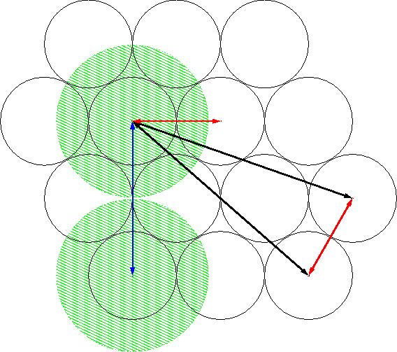
Figure 2: Hexagonal close packed configuration for station centres. The black circles have a radius, $r_{full}$, equal to half the distance between adjacent station centres and all the elements within this area receive their full weight in the beam formation process. The green filled circles have radius equal to $\sqrt{3}r_{full}$ and indicated the full extent of the area over which elements will contribute to this particular station beam. Red arrows shows one of the baselines between adjacent stations which will be discarded before imaging. The shortest legitimate baseline occurs between stations whose green circles are adjacent to each other and do not share any elements and the blue line shows as example of these. The black baselines are both examples of legitimate baselines — note that both of the baselines between one station and a pair of adjacent stations are legitimate, despite the fact that the baseline between these two is discarded.

The scale of hexagonal close packed configuration is defined by the radius of the circles of which it is comprised, called $r_{full}$ for reasons that will become apparent later.

For sake of comparison, I first consider a “standard” set up in which stations comprise elements within $r_{full}$ of the station centre, which are all uniformly weighted during beam forming. The problems with such a solution include:

• The overall filling factor of the aperture array will be reduced by

• There are areas between the stations that are not used by any stations. It would be wasteful to deploy elements in these areas given that they would not be used, but the existence of these “voids” has the following implications:

  • It will be impossible to implement the flexible station size option proposed by the LFAA consortium [4] since these stations would contain void areas not populated by elements resulting in a very poor station beam. Note that for the same reason beam forming large areas for ionospheric calibration (see e.g. [9]) would also be problematic.

  • [8] find that the beam pattern for individual elements taking into account cross-coupling can be well approximated by simulating the response assuming that the elements sit in a semi-infinite sea of elements. Elements located at the edge of stations adjacent to voids will have a significantly different response and this will lead to a poorly known overall station beam.

• The sharp cut off in station illumination will result in a beam pattern will have very strong sidelobes, with strong implications for the possible dynamic range achievable by the telescope (see e.g. [1] for further discussion).

By contrast, in the shared-element configuration, stations are formed from elements within a larger radius greater, and here I consider a scenario in which all those elements with $\sqrt{3}r_{full}$ will contribute. However, those within $r_{full}$ will be added with full weight during beam formation while those beyond will be apodised with a Hanning window function (see Figure 3) i.e.

$$w =1 r\leq r_{full}$$ (1)

$$w =\frac{1}{2}\left(1+\cos{\left(\frac{\pi\left(r-r_{full}\right)}{\left(\sqrt{3}-1\right)r_{full}}\right)}\right)\quad r_{full}\leq r\leq\sqrt{3}r_{full}$$ (2)

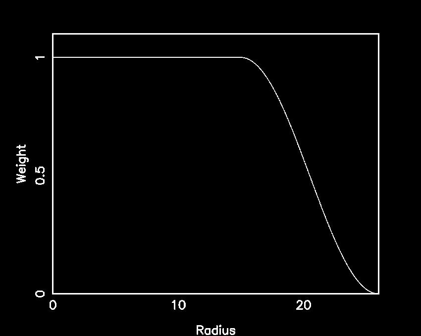
Figure 3: Hanning tapered radial station weighting function (see eqn 1).

Therefore the signals from individual elements will be included in multiple different station beams (see Figure 4); on average they will appear in $3\sqrt{3}/2$. There are no voids in this configuration, so all the problems with the uniformly weighted configuration disappear.

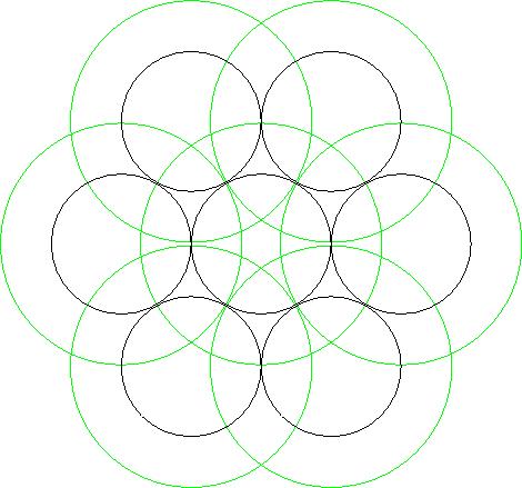
Figure 4: Diagram showing the degree of overlap between stations and that individual elements will therefore be included in multiple different station beams

The possibility therefore exists that visibilities could be formed between stations which incorporate common elements in common. This would give rise to autocorrelation type terms appearing in the visibilities; this is undesirable. Therefore any visibilities formed from stations where the baseline length is less than $2\sqrt{3}r_{full}$ must be discarded — examples of these baselines appear in red and only occur between adjacent stations in the hexagonal close packed configuration. Approximately $3N$ of the $N(N-1)/2$ baselines between the $N$ stations are discarded for this reason. The shortest remaining baselines (hereafter referred to as “legitimate” baselines) occur between stations whose total extent (indicated by the green circles) are adjacent to each other and do not share any elements. However, both of the baselines between one station and a pair of adjacent stations are legitimate, despite the fact that the baseline between these two is discarded.

2.1 Benefits

• The tapering function greatly improves the station sidelobes, which will therefore suppress the effects of bright sources far from the field centre and so in turn improve imaging and calibration, see Figure 5.

• With no voids, the element filling factor in the core is maximised and depends only upon the inter-element spacing.

• A flexible station size now becomes feasible; even if this is not chosen for Phase 1 of the SKA, a flexible station configuration is an attractive upgrade path as beam former technology becomes cheaper, but a configuration with voids will prevent this from being possible to implement.

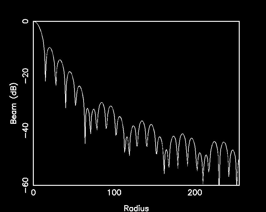
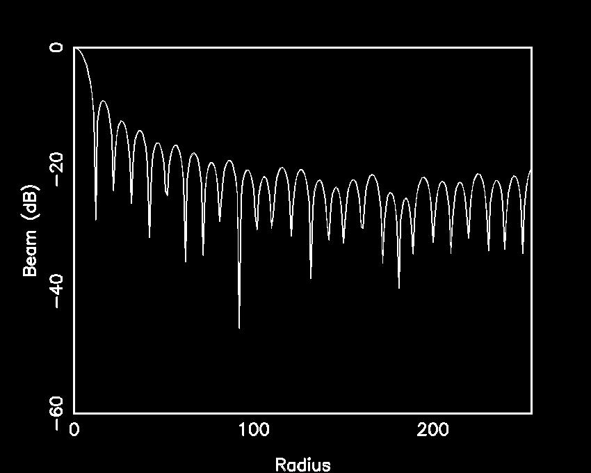
Figure 5: Plot which shows on the left the beam pattern for a (filled) station using the weighting function in eqn 1; and on the right a uniformly weighted circular station.

2.2 Disadvantages

• The beamformer will be more complicated: element signals will be required by more than one station beamformer and the total number of data points to be summed will increase by $3\sqrt{3}/2$.

• The shortest baseline, which determines the maximum angular scale sampled by the telescope, will be $\sqrt{3}$ times longer than that achieved by a configuration where elements are not shared.

2.3 Noise considerations

Compared to a telescope with circular stations of radius $r_{full}$, the proposed configuration has much the same number of baselines (apart from those that are discarded) but a significantly larger collecting area per station; so it is tempting to conclude that this implies an improvement in the sensitivity, but this is not the case. The reason for this is that the visibilities formed from baselines such as the black ones those shown in Figure 2 (hereafter known as “non-independent” baselines) are significantly correlated and so the noise level will not decrease as $\sqrt{n}_{baselines}$; this is discussed further in Section 2.4. There will in fact be a degradation in the maximally achievable sensitivity resulting from the fact that some elements receive more weight than others due to their position. The extent to which this is a problem can be judged from the summed weights, which should ideally be uniform; see Figure 6.

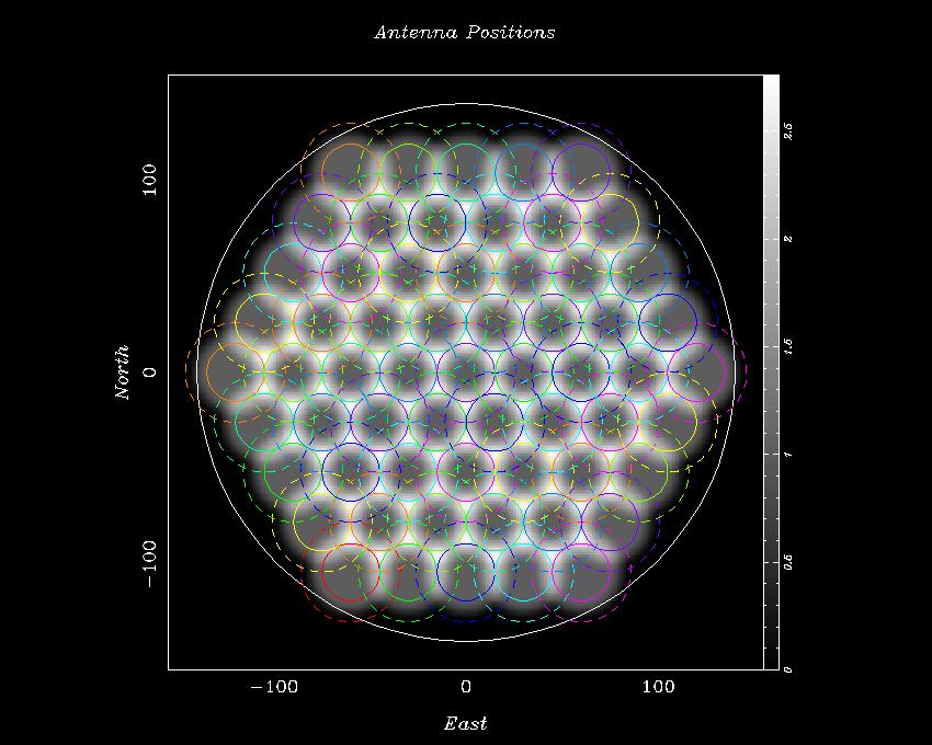
Figure 6: Plot showing the sum weights for a hexagonally close packed configuration of stations using the individual station weights according to Eqn 1. The regions of very high weight arise from regions where 3 stations contribute with just short of full individual weight.

2.4 Visibility correlations

As stated above, visibilities from non-independent baselines such as the black ones those shown in Figure 2 are significantly correlated. However, this is not necessarily a problem. It is always the case that two visibilities will be correlated when there is overlap between their uv-positions on being convolved by the aperture illumination function, because they are sampling a common region of the underlying uv-plane. This correlation between the signals must be accounted for in the covariance matrix when analysing the data in the uv-plane, but the thermal noise is usually assumed to be diagonal. However, for these non-independent baselines, there will also be a correlated component to their noises, which must included in the covariance matrix. This idea is further illustrated in Figure 7. The signal from each station can be considered to be the sum of the voltages from each of its comprising elements. Therefore the visibility formed by the correlation of the two stations is the sum of all the possible products between the two stations. The visibility is therefore a weighted sum of the values in the uv-plane within a patch defined by the convolution of the two station areas (i.e. the aperture illumination function). The non-independent baselines will therefore share some of these product components between individual elements. The result will be that these components will be upweighted with respect to the rest. This is therefore equivalent in standard interferometry to arbitrarily upweighting certain visibilities in the uv-plane and will therefore lead to a sub-optimal signal-to-noise but will not introduce biases.

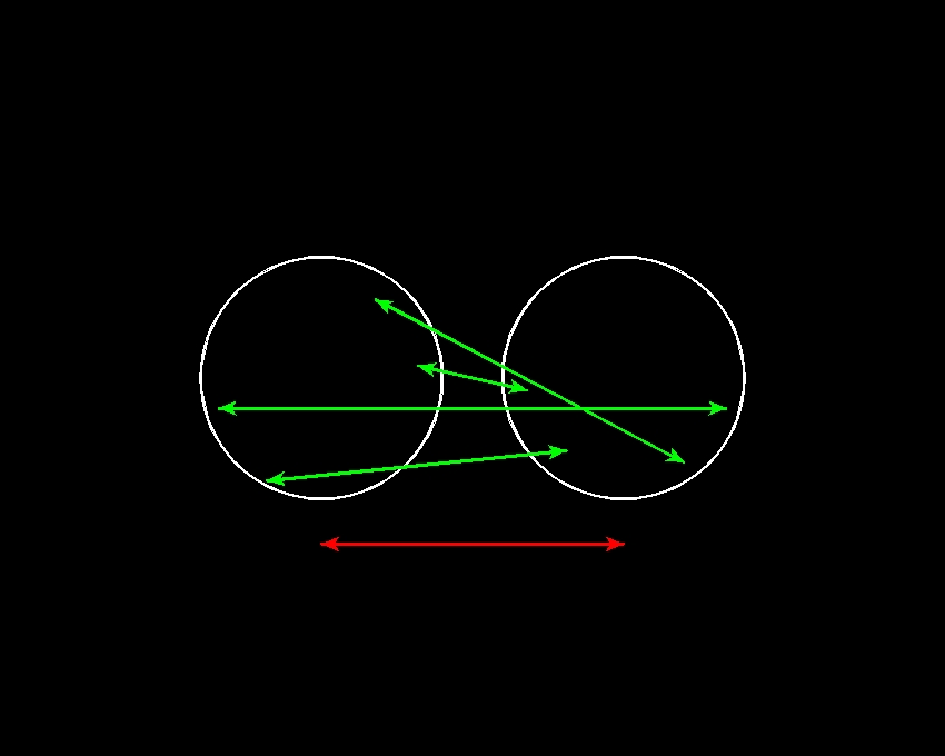
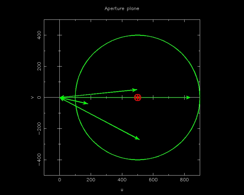
Figure 7: The lefthand plot shows 2 stations and some of the individual baselines that could be formed from correlating elements within each. These baselines are then also shown in the righthand plot in the uv-plane together with the extent of the aperture illumination function for the correlation of the two stations. The redarrow shows the baseline between the centres of the two stations and the redpoint show the corresponding uv position in the aperture plane.

3 Modifications to the shared element configuration

3.1 Randomised station positions

Using a hexagonal close packed configuration gives rise to a large number of redundant baselines, which will be poor for filling of the uv-plane and hence for imaging. Also, since these redundant baselines will have somewhat different station beam patterns due to the random distribution of elements, the level of redundancy is unlikely to be useful for calibration. Therefore a certain amount of reduction in filling factor and a randomisation of the station centres may be valuable.

3.2 Different apodisation functions

Figure 6 shows that some elements are significantly upweighted with respect the mean which will degrade the overall sensitivity of the telescope. Randomising the station centres may alleviate this problem to a certain extent. However, adopting a different weighting function should also be considered; plots for a tapered Gaussian weight function of the same extent are shown in Figure 8. The results look attractive but an optimising the weighting function has not been attempted in this paper.

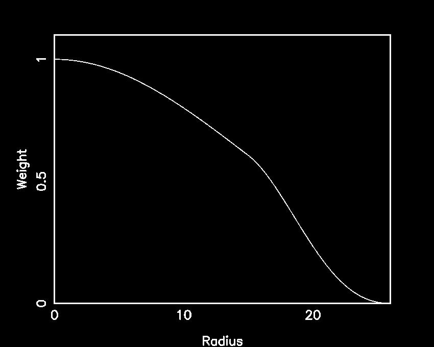
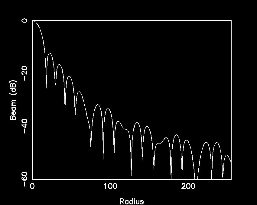
Figure 8: Plots for a tapered Gaussian station weighting function. From top left: the radial weighting function itself; the associated beam response; the sum weights for a hexagonally close packed configuration of stations.

Another possible way forward would be to extend the extent of the tapered region for each station, for example having a Hanning window out to say $2r_{full}$. The disadvantages of implementing this are:

• Increased complexity for the beam former.

• Increased number of baselines that must be rejected since the component stations share elements.

One final possibility that should be considered is whether one needs a “guard area” between adjacent stations whose signals are correlated, since there will certainly be cross-coupling between adjacent elements leading to auto-correlation terms appearing in the visibilities (even if these are significantly downweighted).

3.3 Apodisation through thinning

Apodisation can be achieved either through downweighting of outlying elements in an element or through reducing the density of the elements as a function of radius (i.e. thinning) and weighting them all equally. Downweighting of outlying elements will produce the better beam pattern, but outside the core it will be wasteful of element collecting area, so thinning may be a good compromise; it will certainly give a better beam pattern than a uniformly weighted, uniformly dense, circular station.

4 Limits to the utility of apodisation

Apodisation certainly improves the inner regions of the station beam, but some far-out sidelobes are not suppressed by this method. The reason for this can be seen through an understanding of what generates the various features in the station beam and is argued below in a somewhat pedagogical fashion; experts may wish to skip to Section 5.

4.1 Understanding the station beam of an aperture array

Consider an aperture array of infinite extent, comprised of mono-chromatic elements with delta function receiving area, configured in a hexagonal close packed arrangement and beam formed with equal weights and zero phase offsets. The Fourier transform of this configuration is the voltage station beam of the an array and will be a set off hexagonally close packed delta functions of equal amplitude distributed over an infinite extent (see Figure 9, top. Note that these illustrative figures are simulated with 9000 rather than an infinite number of elements and some non-ideal features are generated). This can be thought of as a main beam pointing towards the zenith and then sidelobes (hereafter “far-out sidelobes” for reasons that will become apparent) arranged in a hexagonal pattern around this. If one reduces the distance (in wavelengths) between elements the distance between the sidelobes of the beam pattern increases, and vice versa.

If one now randomises the configuration while maintaining a minimum spacing between elements the far-out sidelobes become a circularised band with amplitude that is lower than that of the zenith beam and that falls off going to longer radius (see Figure 9, bottom). The radii of these bands from the main lobe is determined by the mean inter-element spacing and the thickness of the band by the distribution of distances to nearest element neighbours (see Figure 10). The main beam is still a delta function (this is not quite apparent in the plots since a finite simulation was used).

Replacing the delta function receiving area of the elements with a Gaussian is equivalent to convolving the station illumination function with the Gaussian. The effect on the Fourier transform i.e. the station beam is therefore to multiply by a Gaussian (see Figure 11). This can be though of as incorporating the angular response pattern of the element, which suppresses the sidelobes.

Finally, one can produce a realistic station configuration with a finite number of elements by multiplying the infinite extent array by a finite function e.g. a circular tophat. The effect on the station beam is therefore to convolve with the Fourier transform of this finite function. For a uniformly weighted circular station, this will result in the main beam delta function being replaced by a function with strong, “near-in” sidelobes (see Figure 12, top). If apodisation is applied, these near-in sidelobes can be suppressed, as discussed in Section 2 (also see Figure 12, bottom). The far-out sidelobes are also convolved with this same function, but this will not lead to any significant suppression. Note that the other, independent, effect of reducing the number of elements within a station is to increase the strength of the far sidelobes.

These near-in and far-out sidelobes therefore have different physical origins. The near-in sidelobes are due to the station size, $D$ and therefore appear at an angular scale size proportional to $D/\lambda$. The far-out sidelobes are due to the fact that the station is comprised of individual elements, mean spacing $d$, and therefore appear at an angular scale size proportional to $d/\lambda$. Since $D\approx d\sqrt{N}$, where $N$ is the number of elements per station, then the number of near-in sidelobes before the first far-out sidelobe is proportional to $\sqrt{N}$. Clavier et al. [2] present a more sophisticated analysis of this phenomenon (using the terms “aperture-type” and “non-coherent” sidelobes) and find that the number of sidelobes inside the far-out sidelobes is well approximated by $0.3\sqrt{N}$. They also find that the power in the far sidelobes goes down as $N$.

Therefore implementing an apodisation to the station illumination can significantly reduce near-in sidelobes, but to first order this will not affect far-out sidelobes. These far-out sidelobes must therefore be suppressed: by the intrinsic element beam pattern; or by time and frequency averaging; or by increasing the number of elements in each station.

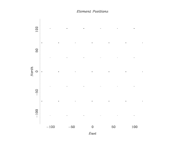
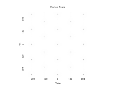
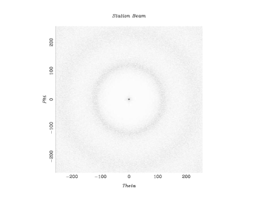
Figure 9: From left: element configuration; station beam; radial station beam power. Top plot show an infinite regular configuration of delta function elements; bottom plots show a randomised configuration with the same mean inter-element spacing.

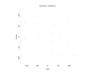
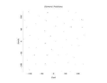
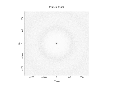
Figure 10: Plots as in Figure 9. Top plots show results for randomised configuration where minimum spacing is 85% of the mean spacing; bottom plots where it is 75% with the same mean. Note that the sidelobe falls in the same place but is broadened.

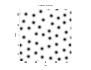
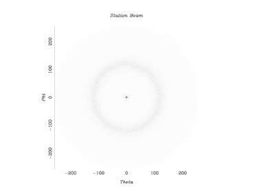
Figure 11: Plots as in Figure 9. Plots show the effect of moving from delta function response elements to a Gaussian response. Note that the sidelobes are suppressed.

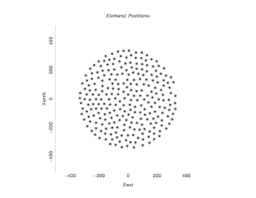
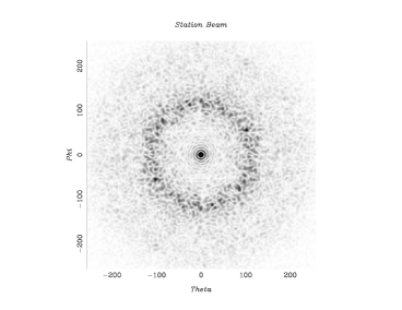
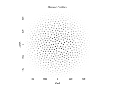
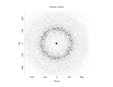
Figure 12: Plots as in Figure 9. The top plot show the effect of moving to a finite sized station; note that the inner beam is now convolved with a function giving strong sidelobes. The bottom plot shows a finite but apodised station which has much suppressed near-in sidelobes.

5 Station configuration within the core

The Baseline Design envisages that the core of SKA-low will be close to miximally packed within the inner 250m radius with the density of stations then dropping off as a Gaussian. There will be 374 stations with 500m and 647 within 1km. Station positions are randomised within this area. This gives a configuration such as shown in Figure 13. Here I consider a different configuration within the inner 1km radius which gives the same density of stations as a function of radius, but has some features which may give important advantages.

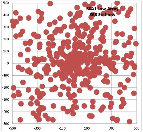
Figure 13: Configuration proposed in the Baseline Design (Dewdney et al.) with a fully filled central region and then a random distribution of stations with a decreasing density.

The new configuration is again fully filled in the central 200m but then implements the density drop with radius with fully filled spiral arms (whose thickness drops with radius) as shown in Figures 14 and 15; in the former the station positions have undergone randomisation while in the latter they are based on a regular grid. The difference between these two variants are discussed later. The configuration has been tailored to give approximately the desired number of stations within each radial annulus as shown in Figure 16 These configurations offer the following possible advantages:

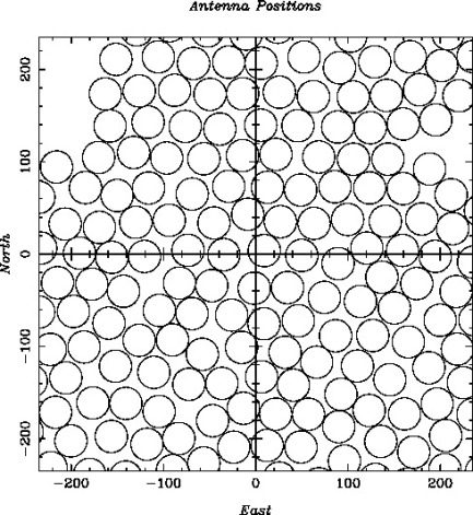
Figure 14: Alternative proposed configuration where the reduction in radial station density is implemented though spiral arms, but within which the elements are fully filled. Station positions have been randomised. The righthand plot shows a close up of the inner region.

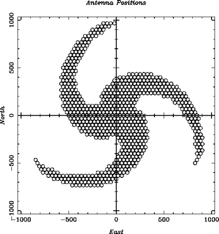
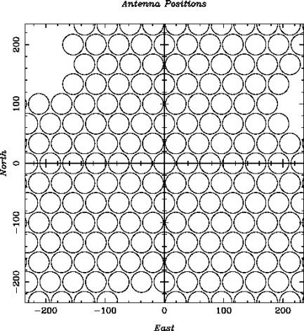
Figure 15: Alternative proposed configuration where the reduction in radial station density is implemented though spiral arms, but within which the elements are fully filled. Station positions have are based on a regular hexagonal close packed grid. The righthand plot shows a close up of the inner region

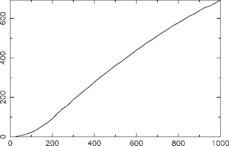
Figure 16: Cumulative number of stations against radius for the configuration shown in Figure 14. There are 361 stations within 500m radius and 691 stations within 1km.

• Expansion to SKA2. In SKA2 the density of stations with radius will be increased dramatically and the fully filled region of the core will be expanded. With the baseline design configuration shown in Figure 13, accessing the site for a new station, bringing in equipment and installing it will be challenging amongst the existing stations. Adding to the configuration shown in Figure 14 will be considerably easier. In addition, just beyond the fully filled region of the Phase 1 core the density of stations will be so high that it will be close to impossible to find a 35m diameter site in which to locate a new station; this is shown in Figure 17. Finally, access for maintenance will be considerably easier with this spiral arm configuration.

• Variable sized stations. The proposed design from the AA consortium [4] envisages a flexible approach to station size, with possible diameters ranging from 20m to 100m. This approach would fail beyond the fully filled region in the Baseline Design configuration since station sizes are defined when they are deployed — there are no more antenna beyond the station edge to allow for the desired flexible approach. In the proposed configuration the spiral arms are fully filled and so allow for the possibility for redefinition of stations dynamically.

• Overlaping, apodised stations. As described in Section 2 document there are many potential benefits to the station beam shape and calibratability that could be realised through defining overlapping stations where a radial weighting is applied during beamforming to suppress far sidelobes. Similarly to above, this does require a fully filled configuration such as would be provided by the proposed filled spiral arms.

• Number of short baselines. Since the spiral arms are fully filled they will generate a reasonable number of shortest possible baselines which are critical for brightness sensitivity on the largest angular scales, see Figure 18. This is important for the EoR experiment.

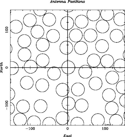
Figure 17: A realisation of Baseline Design configuration just outside the fully filled region with a filling factor of approximately 2 lower than fully filled. Increasing the density of the AA for SKA2 will cause significant logistical problems. In addition, it will be difficult to identify possible sites for new 35m stations.

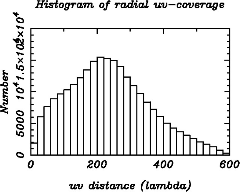
Figure 18: Histogram of number of baselines (measured in lambda assuming an observing frequency of 100 MHz) generated by the configuration shown in Figure 14.

The main disadvantage to the proposed configuration is that the uv-coverage will necessarily be less uniform that that generated by the Baseline Design configuration. However, since there are 647 station the coverage can still be excellent as long the configuration is randomised. Figure 19 shows the snapshot uv-plane coverage corresponding to Figure 14, with a close up of the inner region. The uv-coverage therefore looks very good, but could of course be improved further with earth-rotation synthesis. For comparison, Figure 20 shows the inner part of the uv-plane for the un-randomised configuration shown in Figure 15.

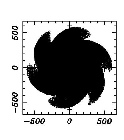
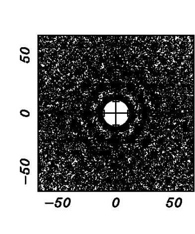
Figure 19: Snapshot coverage of the uv-plane for the configuration shown in Figure 14 assuming an observing frequency of 100 MHz. The righthand plot shows a close up view of the centre of the aperture plane.

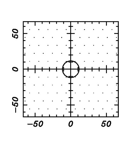
Figure 20: Snapshot coverage of the uv-plane for the configuration shown in the righthand plot of Figure 14 assuming an observing frequency of 100 MHz. The regular grid adopted results in very high redundancy of baselines and so a correspondingly poor coverage of the uv-plane. The circle radius approx 10 lambda is the size of the aperture illumination function.

References

- [1] Braun R., 2013, A&A 551, A91
- [2] Clavier, T. et al., 2013, IEEE Transactions on Antennas and Propagation, 99, 1
- [3] Dewdeney, P.E., 2013, SKA-1 System Baseline design, SKA-TEL-SKO-DD-001-1_BaselineDesign1.
- [4] Faulkner, A., 2013, Low Frequency Aperture Array Technical Description, AADC-TEL.LFAA.SE.MGT-AADC-PL-002
- [5] Gonzalez-Ovejero, D., 2011, IEEE International Symposium on Antennas and Propagation, 1762
- [6] de Lera Acedo, E., 2011, IEEE Transactions on Antennas and Propagation, vol. 59, 1808
- [7] de Lera Acedo, E., 2012, International Conference on Electromagnetics in Advanced Applications, 353.
- [8] de Lera Acedo, E., et al., 2011 International Conference on Electromagnetics in Advanced Applications, 390.
- [9] Wijnholds, S. J., Bregman J. D. and van Ardenne, A., 2011, Radio Science, 46, RS0F07