A Generalized Parallel Replica Dynamics

Abstract.

Metastability is a common obstacle to performing long molecular dynamics simulations. Many numerical methods have been proposed to overcome it. One method is parallel replica dynamics, which relies on the rapid convergence of the underlying stochastic process to a quasi-stationary distribution. Two requirements for applying parallel replica dynamics are knowledge of the time scale on which the process converges to the quasi-stationary distribution and a mechanism for generating samples from this distribution. By combining a Fleming-Viot particle system with convergence diagnostics to simultaneously identify when the process converges while also generating samples, we can address both points. This variation on the algorithm is illustrated with various numerical examples, including those with entropic barriers and the 2D Lennard-Jones cluster of seven atoms.

1. Introduction

An outstanding obstacle for many problems modeled by in situ molecular dynamics (MD) is the vast separation between the characteristic time for atomic vibrations ($10^{-15}$ s), and the characteristic time for macroscopic phenomena ($10^{-9}$ – $10^{-3}$ s). At the heart of this scale separation is the presence of metastable regions in the configuration space of the problem. Examples of metastable configurations include the defect arrangement in a crystal or the conformation of a protein. Such metastability may be due to either the energetic barriers of a potential energy driving the problem or to the entropic barriers arising from steric constraints. In the first case (energetic barriers), metastability is due to the system needing to pass through a saddle point which is higher in energy than the local minima to get from one metastable region to another. In the second case (entropic barriers), metastability is due to the system having to find a way through a narrow (but not necessarily high energy) corridor to go from one large region to another (see Section 5.3 below for an example with entropic barriers)

Motivated by the challenge of this time-scale separation, A.F. Voter proposed several methods to conquer metastability in the 1990s: Parallel Replica Dynamics (ParRep), Temperature Accelerated Dynamics (TAD) and Hyperdynamics (Hyper), [31, 33, 38, 37, 39, 40]. These methods were derived using Transition State Theory and intuition developed from kinetic Monte Carlo models, as the latter describes the hopping dynamics between metastable regions. Indeed, the aim of all these algorithms is to efficiently generate a realization of the discrete-valued jump process amongst metastable regions. The main idea is that the details of the dynamics within each metastable region are not essential to our physical understanding. Rather, the goal should be to get the correct statistics of the so-called state-to-state dynamics, corresponding to jumps amongst the metastable regions. This is nontrivial in general for two reasons: (i) the original dynamics projected onto the state-to-state dynamics are not Markovian; (ii) the parameters (transition rates) of the underlying state-to-state dynamics are unknown.

In recent mathematical studies of these approaches, it has been shown that these three algorithms take advantage of quasi-stationary distributions (QSDs) associated with the metastable states, see [1, 24, 25, 32]. Crudely, the QSD corresponds to the distribution of the end points of trajectories conditioned on persisting in the region of interest for a very long time. This mathematical formalization clarifies the fundamental assumptions under which the algorithms will be accurate and also broadens their applicability. Indeed, one aim of this paper is to propose a modification of the original ParRep algorithm that will allow for states to be defined by generic partitions of configuration space. This bears some resemblance to milestoning, which also allows more general partitions of configuration space, [22, 36]. Therefore, we will not refer to “basins of attractions” or “metastable regions”, but rather simply to “states”. The only requirement is that these states define a partition of the configuration space. The boundary at the interface between two states is called the dividing surface.

Briefly (this is detailed in Section 2.3 below), ParRep works by first allowing a single reference trajectory to explore a state. If the trajectory survives for sufficiently long, its end point will agree, in law, with the aforementioned QSD. One thus introduces a decorrelation time, denoted $t_{\mathrm{corr}}$, as the time at which the law of the reference process will have converged to the QSD. Provided the reference process survives in the state up till $t_{\mathrm{corr}}$, it is replaced by an ensemble of $N$ independent and identically distributed replicas, each with an initial condition drawn from the QSD. The first replica to escape is then followed into the next state. As the replicas evolve independently and only a first escape is desired, they are readily simulated in parallel, providing as much as a factor of $N$ speedup of the exit event. Thus, there are two practical challenges to implementing ParRep:

• Identifying a $t_{\mathrm{corr}}$ at which the law of the reference process is close to the QSD.

• Generating samples from the QSD from which to start the replicas.

In the original algorithm, $t_{\mathrm{corr}}$ is a priori chosen by the user, as the states are defined so that an approximation of the time required to get “local equilibration within the state” is available. Such a value can be estimated in the case of energetic barriers at sufficiently low temperature using harmonic transition state theory. But in the case of entropic barriers, there is, in general, no simple estimate; see, however, [23] for an example where ParRep was applied to an entropic barrier as an estimate of $t_{\mathrm{corr}}$ was available. In the original algorithm, the sampling of the QSD is done using a rejection algorithm, which will be inefficient if the state does not correspond to a metastable region for the original dynamics. Indeed, this will degenerate in the long time limit, as the trajectories will always exit. In this work, we propose an algorithm addressing both points, based on two ingredients:

• The use of a branching and interacting particle system called the Fleming-Viot particle process to simulate the law of the process conditioned on persisting in a state, and to sample the QSD in the longtime limit.

• The use of Gelman-Rubin statistics in order to identify the correlation time, namely the convergence time to a stationary state for the Fleming-Viot particle process.

As we state below, this modified version of ParRep, presented below in Section 3, relies on assumptions (see (A1) and (A2) below) which would require more involved analysis to fully justify. We demonstrate below in a collection of numerical experiments that this modified algorithm gives results consistent with direct simulations. We observe speedup factors up to ten in our test problems where $N=100$ replicas were used. The aim of this paper is to present new algorithmic developments, and not to explore the mathematical foundations underpinning these ideas.

Though we focus on the ParRep algorithm, since it is the most natural setting for introducing the Fleming-Viot particle process, identifying the convergence to the QSD is also relevant to other problems, including the two other accelerated dynamics algorithms: Hyper and TAD. See [1, 25] for the relevant discussions.

Our paper is organized as follows. In Section 2, we introduce the dynamics of interest, review some properties of the QSD and recall the original ParRep algorithm. In Section 3, we then present the Fleming-Viot particle process and the Gelman-Rubin statistics, which are needed to build the modified ParRep algorithm we propose. Finally, in Section 4 we show the effectiveness and caveats of convergence diagnostics, before exploring the efficiency and accuracy of the modified ParRep algorithm on various test cases in Section 5.

1.1. Acknowledgments

A.B. was supported by a US Department of Defense NDSEG fellowship. G.S. was supported in part by the US Department of Energy Award DE-SC0002085 and the US National Science Foundation PIRE Grant OISE-0967140. T.L. acknowledges funding from the European Research Council under the European Union’s Seventh Framework Programme (FP7/2007-2013) grant agreement no. 614492.

The authors would also like to thank C. Le Bris, M. Luskin, D. Perez, and A.F. Voter for comments and suggestions throughout the development of this work. The authors would also like to thank the referees for their helpful remarks.

2. The Original ParRep and Quasi-Stationary Distributions

2.1. Overdamped Langevin Dynamics

We consider the case of the overdamped Langevin equation

(2.1) $$dX_{t}=-\nabla V(X_{t})dt+\sqrt{2\beta^{-1}}dW_{t}.$$

Here, the stochastic process $(X_{t})_{t\geq 0}$ takes values in $\mathbb{R}^{d}$, $\beta$ is the inverse temperature, $V(x)$ is the driving potential and $W_{t}$ a standard $d$-dimensional Brownian motion. In all that follows, we focus, for simplicity, on (2.1). However, the algorithm we propose equally applies to the phase-space Langevin dynamics which are also of interest. As mentioned in the introduction, for typical potentials, the stochastic process $(X_{t})_{t\geq 0}$ satisfying (2.1) is metastable. Much of its trajectory is confined to particular regions of $\mathbb{R}^{d}$, occasionally hopping amongst them.

Let $\Omega\subset\mathbb{R}^{d}$ denote the region of interest (namely the state), and define

(2.2) $$T=\inf\left\{t\geq 0\mid X_{t}\notin\Omega\right\}$$

to be the first exit time from $\Omega$, where $X_{0}=x\in\Omega$. The point on the boundary, $X_{T}\in\partial\Omega$, is the first hitting point. The aim of accelerated dynamics algorithms (and ParRep in particular) is to efficiently sample $(T,X_{T})$ from the exit distribution.

2.2. Quasi-stationary Distributions

In order to present the original ParRep algorithm, it is helpful to be familiar with quasi-stationary distributions (QSD). For more details about quasi-stationary distributions, we refer the reader to, for example,  [7, 8, 9, 26, 27, 34, 10]. Reference [24] gives self-contained proofs of the results below.

Consider a smooth bounded open set $\Omega\subset\mathbb{R}^{d}$, that corresponds to a state. By definition, the quasi-stationary distribution $\nu$, associated with the dynamics (2.1) and the state $\Omega$, is the probability distribution, with support on $\Omega$, satisfying, for all (measurable) $A\subset\Omega$ and $t\geq 0$,

(2.3) $$\begin{split}\nu(A)=\frac{\int\mathbb{P}^{x}\left[X_{t}\in A,T>t\right]\nu(dx)}{\int\mathbb{P}^{x}\left[T>t\right]\nu(dx)}&=\frac{\mathbb{P}^{\nu}\left[X_{t}\in A,T>t\right]}{\mathbb{P}^{\nu}\left[T>t\right]}=\mathbb{P}^{\nu}\left[X_{t}\in A\mid T>t\right].\end{split}$$

Here and in the following, we indicate by a superscript the initial condition for the stochastic process: $\mathbb{P}^{x}$ indicates that $X_{0}=x$ and $\mathbb{P}^{\nu}$ indicates that $X_{0}$ is distributed according to $\nu$. In our setting, it can be shown that $\nu$ exists and is unique.

The QSD enjoys three properties. First, it is related to an elliptic eigenvalue problem. Let $L$ be the infinitesimal generator of (2.1), defined by, for any smooth function $v:\mathbb{R}^{d}\to\mathbb{R}$,

(2.4) $$Lv=-\nabla V\cdot\nabla v+\beta^{-1}\Delta v.$$

The operator $L$ is related to the stochastic process through the following well-known result: if the function $u:\mathbb{R}^{+}\times\Omega\to\mathbb{R}$ satisfies the Kolmogorov equation:

(2.5) $$\left\{\begin{aligned} \partial_{t}u&=Lu=-\nabla V\cdot\nabla u+\beta^{-1}\Delta u,\quad\text{for $t>0$, $x\in\Omega$},\\ u(t,x)&=f(x)\quad\text{for $t>0$, $x\in\partial\Omega$},\\ u(0,x)&=u_{0}(x)\quad\text{for $x\in\Omega$},\end{aligned}\right.$$

then $u$ admits the probabilistic representation formula (Feynman-Kac relation):

(2.6) $$u(t,x)=\mathbb{E}^{x}\left[u_{0}(X_{t})1_{T>t}\right]+\mathbb{E}^{x}\left[f(X_{T})1_{T\leq t}\right].$$

Recall that $T$ defined by (2.2), is the first exit time of $X_{t}$ from $\Omega$. Provided $\Omega$ is bounded with sufficiently smooth boundary and $V$ is smooth, $L$ has an infinite set of Dirichlet eigenvalues and orthonormal eigenfunctions

(2.7) $$L\varphi_{j}=-\lambda_{j}\varphi_{j},\quad\varphi_{j}|_{\partial\Omega}=0,\quad j=1,2,\ldots$$

Here, the eigenfunctions are orthonormal with respect to the invariant measure restricted to $\Omega$:

$$\frac{\int_{\Omega}\varphi_{j}(x)\varphi_{k}(x)\exp(-\beta V(x))dx}{\int_{\Omega}\exp(-\beta V(x))dx}=\delta_{jk},\quad\forall j,k=1,2,\ldots$$

The eigenfunction associated with the lowest eigenvalue is signed, and, taking it to be positive, the QSD is

(2.8) $$\nu(dx)=\frac{\displaystyle\varphi_{1}(x)e^{-\beta V(x)}dx}{\displaystyle\int_{\Omega}\varphi_{1}(x)e^{-\beta V(x)}dx}.$$

While this expression is explicit in terms of $\varphi_{1}$ and $V$, since the problem is posed in $\mathbb{R}^{d}$ with $d$ large, it is not practical to sample the QSD directly by first computing $\varphi_{1}$.

The second property associated to the QSD is that for all $t\geq 0$ and $A\subset\partial\Omega$:

(2.9) $$\begin{split}\mathbb{P}^{\nu}\left[X_{T}\in A,T>t\right]&=\mathbb{P}^{\nu}\left[T>t\right]\,\mathbb{P}^{\nu}\left[X_{T}\in A\right]\\ &=\left(e^{-\lambda_{1}t}\right)\,\left(\int_{A}-\frac{1}{\beta\lambda_{1}}\frac{\nabla\varphi_{1}e^{-\beta V}\cdot{\bf n}}{{\int_{\Omega}\varphi_{1}(x)e^{-\beta V(x)}dx}}d{S}\right),\end{split}$$

where $dS$ is the surface Lebesgue measure on $\partial\Omega$ and ${\bf n}$ the unit outward normal vector to $\Omega$. Thus, the first hitting point and first exit time are independent, and exit times are exponentially distributed. These two properties will be one of the main arguments justifying ParRep. As explained in [24], they are consequences of (2.6) and (2.8).

The third property of the QSD also plays an important role in ParRep. Let us again consider $X_{t}$ satisfying (2.1) with $X_{0}\sim\mu_{0}$ ($\mu_{0}$ with support in $\Omega$). Define the law of $X_{t}$, conditioned on non-extinction as:

(2.10) $$\mu_{t}(\bullet)=\frac{\mathbb{P}^{\mu_{0}}\left[X_{t}\in\bullet,T>t\right]}{\mathbb{P}^{\mu_{0}}\left[T>t\right]}=\mathbb{P}^{\mu_{0}}\left[X_{t}\in\bullet\mid T>t\right].$$

One can check that

(2.11) $$\mu_{t}(v_{0})=\mathbb{E}^{\mu_{0}}\left[v_{0}(X_{t})\mid T>t\right]=\frac{\int_{\Omega}v(x,t)\mu_{0}(dx)}{\int_{\Omega}\bar{v}(x,t)\mu_{0}(dx)},$$

where $v$ solves (2.5) with initial condition $v(0,x)=v_{0}(x)$ and boundary conditions $v|_{\partial\Omega}=0$ while $\bar{v}$ solves (2.5) with initial condition $\bar{v}(0,x)=1$ and boundary conditions $\bar{v}|_{\partial\Omega}=0$. Through eigenfunction expansions of the form

(2.12) $$v(t,x)=\sum_{k=1}^{\infty}e^{-\lambda_{k}t}\varphi_{k}(x)\int v_{0}(y)\varphi_{k}(y)\frac{e^{-\beta V(y)}}{\int e^{-\beta V}}dy$$

we obtain: for $t$ sufficiently large, the total variation norm can be bounded as

(2.13) $$\left\|\mu_{t}-\nu\right\|_{\mathrm{TV}}\equiv\sup_{\left\|f\right\|\leq 1}\left|\int f(x)\mu_{t}(dx)-\int f(x)\nu(dx)\right|\leq C(\mu_{0})e^{-(\lambda_{2}-\lambda_{1})t}.$$

In the above expression, $\left\|f\right\|=\left\|f\right\|_{L^{\infty}(\Omega)}$. This shows that if the process remains in $\Omega$ for a sufficiently large amount of time (typically of the order of $1/(\lambda_{2}-\lambda_{1})$), then its law at time $t$ is close to the QSD $\nu$.

Since we are interested in ensuring that the state to state dynamics are accurate, we observe that (2.13) implies agreement of the exit distribution of $(T,X_{T})$ in total variation norm between processes initially distributed according to $\mu_{t}$ and $\nu$. Indeed, starting from the probability measure $\mu_{t}$, given any measurable $g:\mathbb{R}^{+}\times\partial\Omega\to\mathbb{R}$, we see that exit distribution observables can be reformulated as observables on $\Omega$ against $\mu_{t}$:

(2.14) $$\mathbb{E}^{\mu_{t}}\left[g(T,X_{T})\right]=\int\underbrace{\mathbb{E}^{x}\left[g(T,X_{T})\right]}_{\equiv G(x)}\mu_{t}(dx)=\int G(x)\mu_{t}(dx).$$

Therefore,

(2.15) $$\sup_{\left\|g\right\|\leq 1}\left|\mathbb{E}^{\mu_{t}}\left[g(T,X_{T})\right]-\mathbb{E}^{\nu}\left[g(T,X_{T})\right]\right|\leq\left\|\mu_{t}-\nu\right\|_{\mathrm{TV}}\leq C(\mu_{0})e^{-(\lambda_{2}-\lambda_{1})t},$$

where $\left\|g\right\|=\left\|g\right\|_{L^{\infty}(\mathbb{R}^{+}\times\partial\Omega)}$. Thus, convergence of $\mu_{t}$ to $\nu$ implies agreement of the exit distributions, starting from $\mu_{t}$ and $\nu$.

We are now in position to introduce the original ParRep algorithm.

2.3. Parallel Replica Dynamics

The goal of the ParRep algorithm is to rapidly generate a physically consistent first hitting point and first exit time for each visited state. Information about where, precisely, the trajectory is within each state will be sacrificed to more rapidly obtain this information.

In the following, we assume that we are given a partition of the configuration space $\mathbb{R}^{d}$ into states, and we denote by $\Omega$ one generic element of this partition. We also assume that we have $N$ CPUs available for parallel computation.

The original ParRep algorithm [39] is implemented in three steps, repeated as the process moves from one state to another. It requires the specification, a priori, of two times to equilibrate to each state, $t_{\mathrm{corr}}$ and $t_{\mathrm{phase}}$. Let us consider a single reference process, $X_{t}^{\mathrm{ref}}$, with $X_{0}^{\mathrm{ref}}\sim\mu_{0}$ evolving under (2.1), and set the simulation clock, corresponding to the physical time, to zero, $t_{\mathrm{sim}}=0$. The simulation clock $t_{\mathrm{sim}}$ will be updated during the algorithm.

Decorrelation Step:

Let $\Omega$ denote the state in which $X_{t_{\mathrm{sim}}}^{\mathrm{ref}}$ currently resides. If the trajectory has not left $\Omega$ after running for $t_{\mathrm{corr}}$ amount of time, the algorithm proceeds to the dephasing step, the simulation clock being advanced as

$$t_{\mathrm{sim}}\mapsto t_{\mathrm{sim}}+t_{\mathrm{corr}}.$$

Otherwise a new decorrelation starts from the new state, the simulation clock being advanced as

$$t_{\mathrm{sim}}\mapsto t_{\mathrm{sim}}+T^{\mathrm{ref}},\quad T^{\mathrm{ref}}=\inf\left\{t\geq 0\mid X^{\mathrm{ref}}_{t_{\mathrm{sim}}+t}\notin\Omega\right\}.$$

Dephasing Step:

In this step, $N$ independent and identically distributed samples of the QSD of $\Omega$ are generated. These samples will be distributed over the $N$ CPUs and will be used as initial conditions in the subsequent parallel step. During the dephasing step, the counter $t_{\mathrm{sim}}$ is not advanced.

In the original ParRep, the sampling of the QSD is accomplished by a rejection algorithm. For $k=1,\ldots,N$, generate a starting point $\tilde{X}_{0}^{k}\sim\eta_{0}$ and integrate it under (2.1) until either time $t_{\mathrm{phase}}$ or $\tilde{X}_{t}^{k}$ leaves $\Omega$. Here, $\eta_{0}$ denotes any distribution with support in $\Omega$ (for example, a Dirac mass at the end point of the reference trajectory, after the decorrelation step). If $\tilde{X}_{t}^{k}$ has not exited before time $t_{\mathrm{phase}}$, set the $k$-th replica’s starting point $X_{0}^{k}=\tilde{X}_{t_{\mathrm{phase}}}^{k}$ and advance $k\mapsto k+1$. Otherwise, reject the sample, and start a new trajectory with $\tilde{X}_{0}^{k}\sim\eta_{0}$. Since these samples are independent, they can be generated in parallel.

Parallel Step:

Let the $N$ samples obtained after the dephasing step evolve under (2.1) in parallel (one on each CPU), driven by independent Brownian motions, until one escapes from $\Omega$. Let us denote

$$k_{\star}={\rm argmin}_{k}T^{k}$$

the index of the first replica which exits $\Omega$. During the time interval $[t_{\mathrm{sim}},t_{\mathrm{sim}}+NT^{k_{\star}}]$, the reference process is defined as trapped in $\Omega$. Accordingly, the simulation clock is advanced as

(2.16) $$t_{\mathrm{sim}}\mapsto t_{\mathrm{sim}}+NT^{k_{\star}},\quad$$

The first replica to escape becomes the new reference process. A new decorrelation step now starts, applied to the new reference process with starting point $X^{\mathrm{ref}}_{t_{\mathrm{sim}}}=X^{k_{\star}}_{T^{{k_{\star}}}}$.

The justifications underlying the ParRep algorithm are the following. Using the third property (2.13) of the QSD, it is clear that if $t_{\mathrm{corr}}$ is chosen sufficiently large, then, at the end of the decorrelation step, the reference process is such that $X^{\mathrm{ref}}_{t_{\mathrm{sim}}}$ is approximately distributed according to the QSD. This same property explains why the rejection algorithm used in the dephasing step yields (approximately) $N$ i.i.d. samples distributed according to the QSD, at least if $t_{\mathrm{phase}}$ is chosen sufficiently large. Finally the second property (2.9) justifies the parallel step; since the $N$ replicas are i.i.d. and drawn from the QSD, they have exponentially distributed exit times and thus $\mathbb{P}^{\nu}\left[\min\left\{T^{1},\ldots,T^{N}\right\}>t\right]=\mathbb{P}^{\nu}[T^{1}>Nt]$. Moreover, by the independence property in (2.9), the exit points $X^{k_{\star}}_{T^{{k_{\star}}}}$ and $X^{1}_{T^{1}}$ have the same distribution.

Notice that it is the magnification of the first exit time by a factor of $N$ in the parallel step that yields the speedup in terms of wall clock time. If the partition of the configuration space is chosen in such a way that, most of the time, the stochastic process exits from the state before having reached the QSD (namely before $t_{\mathrm{corr}}$), there is no speedup. In this case, ParRep essentially consists in following the reference process. There is no error, but no gain in performance, and computational resources are wasted. To observe a significant speedup, the partition of the configuration space should be such that most of the defined states are metastable, in the sense that the typical exit time from the state is much larger than the time required to approximate the QSD.

Of course, the QSD is only sampled approximately, and this introduces error in ParRep. The time $t_{\mathrm{corr}}$ (resp. $t_{\mathrm{phase}}$) must be sufficiently large such that $\mathbb{P}^{\mu_{0}}\left[X_{t_{\mathrm{corr}}}^{\mathrm{ref}}\in\bullet\mid T^{\mathrm{ref}}>t_{\mathrm{corr}}\right]\approx\nu$ (resp. such that $\mathbb{P}^{\eta_{0}}\left[X_{t_{\mathrm{phase}}}\in\bullet\mid T>t_{\mathrm{phase}}\right]\approx\nu$). The mismatch between the distributions at times $t_{\mathrm{corr}}$ and $t_{\mathrm{phase}}$, directly, and independently, contribute to the overall error of ParRep; see [32]. Also note that these parameters are state dependent. In view of (2.13), one may think that a good way to choose $t_{\mathrm{corr}}$ and $t_{\mathrm{phase}}$ is to consider a multiple of $1/(\lambda_{2}-\lambda_{1})$. This is unsatisfactory for two reasons. First, it is difficult to numerically compute the spectral gap $\lambda_{2}-\lambda_{1}$ because of the high-dimensionality of the associated elliptic problem. Second, the pre-factors $C(\mu_{0})$ and $C(\eta_{0})$ in (2.13) are also difficult to evaluate, and could be large.

In view of the preceding discussion, ParRep can be applied to a wide variety of problems and for any predefined partition of the configuration space into states provided one has:

• A way to construct an adequate $t_{\mathrm{corr}}$ (or more precisely to assess the convergence of $\mu_{t}$ to $\nu$) for each state;

• A way to sample the QSD of each state.

The aim of the next section is to provide a modified ParRep algorithm to deal with these two difficulties.

3. The Modified ParRep Algorithm

We propose to use a branching and interacting particle system (the Fleming-Viot particle process) together with convergence diagnostics to simultaneously and dynamically determine adequate values $t_{\mathrm{corr}}$ and $t_{\mathrm{phase}}$, while also generating an ensemble of $N$ samples from a distribution close to that of the QSD.

3.1. The Fleming-Viot Particle Process

In this section, we introduce a branching and interacting particle system which will be one of the ingredients of the modified ParRep algorithm. This process is sometimes called the Fleming-Viot particle process [15].

Let us specify the Fleming-Viot particle process; see also the illustration in Figure 1. Let us consider i.i.d. initial conditions $X_{0}^{k}$ ($k\in\{1,\ldots,N\}$) distributed according to $\mu_{0}$, a probability distribution with support in $\Omega$. The process is as follows:

1. Integrate $N$ realizations of (2.1) with independent Brownian motions until one of them, say $X_{t}^{1}$, exits;

2. Kill the process that exits;

3. With uniform probability $1/(N-1)$, randomly choose one of the survivors, $X_{t}^{2},\ldots,X_{t}^{N}$, say $X_{t}^{2}$;

4. Branch $X_{t}^{2}$, with one copy persisting as $X_{t}^{2}$, and the other becoming the new $X_{t}^{1}$ (and thus evolving in the future independently from $X_{t}^{2}$).

We denote this branching and interacting particle process by ${\bf X}_{t,N}=(X_{t}^{1},\ldots,X_{t}^{N})$, and define the associated empirical distribution

(3.1) $$\mu_{t,N}\equiv\frac{1}{N}\sum_{k=1}^{N}\delta_{X^{k}_{t}}.$$

The Fleming-Viot particle process can be implemented in parallel, with each replica $X_{t}^{k}$ evolving on distinct CPUs. The communication cost (due to the branching step) will be small, provided the state under consideration is such that the exit events are relatively rare; i.e., it is metastable.

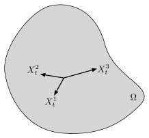
(a) $t_{1}$

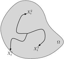
(b) $t_{2}$

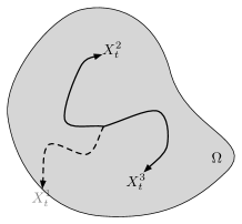
(c) $t_{2}$

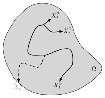
(d) $t_{3}$

Figure 1. The branching & interacting particle system used to sample the QSD in the case $N=3$ at three times: $t_{1}<t_{2}<t_{3}$. The trajectories run independently until one exits, as in (b). The process that has reached the boundary is killed, as in (c). Then a survivor is instantaneously branched to maintain a constant number of trajectories, as in (d).

The Fleming-Viot particle process has been studied for a variety of underlying stochastic processes; see, for example, [15, 29, 13] and the references therein. In [29], the authors prove that for a problem in dimension one, the following relation holds: for any $A\subset\Omega$,

(3.2) $$\lim_{N\to\infty}\mu_{t,N}(A)=\mu_{t}(A).$$

From (2.13) and (3.2), we infer that $\lim_{t\to\infty}\lim_{N\to\infty}\mu_{t,N}(A)=\nu(A)$. This result is anticipated to hold for general dynamics, including (2.1).

The property (3.2) of the Fleming-Viot particle process is instrumental in our modified ParRep algorithm. It will be used in two ways:

• Since an ensemble of realizations distributed according to $\mu_{t}$ can be generated using the Fleming-Viot particle process, we will assess convergence of $\mu_{t}$ to the stationary distribution $\nu$ by applying convergence diagnostics to the ensemble $(X^{1}_{t},\ldots,X^{N}_{t})$. This will give a practical way to estimate the time required for convergence to the QSD in the decorrelation step, by simultaneously running the decorrelation step (on the reference process) and the dephasing step using a Fleming-Viot particle process on $N$ other samples, starting from the same initial condition as the reference process: the decorrelation time is estimated as the time required for convergence to a stationary state for the Fleming-Viot particle process.

• In addition, the Fleming-Viot particle process introduced in the procedure described above gives a simple way to sample the QSD. We use the replicas generated by the modified dephasing step at the time of stationarity.

The modified ParRep algorithm will be based on the two following assumptions on the Fleming-Viot particle process. While we do not make this rigorous, we believe it could be treated in specific cases, and our numerical experiments show consistency with direct numerical simulation.

Assumption (A1):

For sufficiently large $N$, $\mu_{t,N}$ is a good approximation of $\mu_{t}$;

Assumption (A2):

The realizations generated by the Fleming-Viot particle process are sufficiently weakly correlated so as to allow the use of both the convergence diagnostics presented below and the temporal acceleration expression (2.16), which both assume independence.

As already mentioned above, the first assumption is likely satisfied in our setting, though we were not able to find precisely this result in the literature. See [29] for such a result in a related problem.

The second assumption is more questionable. We make two comments on this. First, our numerical experiments show that the modified ParRep algorithm (which is partly based on (A2)) indeed yields correct results compared to direct numerical simulation; thus, the assumption is not grossly wrong, at least in these settings. Second, the correlations introduced by the Fleming-Viot particle process are most likely a concern for problems where the state is only weakly metastable. In truly metastable states, exits will be infrequent, so the correlations amongst the replicas will be weak. For states which are not metastable, the reference process will likely exit before stationarity can be reached, rendering the concern moot. It is therefore in problems between the two cases that practitioners may have some cause for concern.

There are several ways to ameliorate reservations about the second assumption. First, it is known that for such branching and interacting particle systems, a propagation of chaos result holds, [35]. This means that if we run Fleming-Viot with $M\gg N$ processes, then, as $M$ tends to infinity, with $N$ fixed, the first $N$ trajectories in the process become i.i.d. Second, one could run a separate Fleming-Viot particle process for each of the $N$ replicas, retaining only the first trajectory of each of the $N$ i.i.d. Fleming-Viot particle processes. Finally, the Fleming-Viot particle process, together with convergence diagnostics, could be used to identify appropriate values of $t_{\mathrm{phase}}$ and and $t_{\mathrm{corr}}$, as explained below in Section 3.2. This value $t_{\mathrm{phase}}$ could then be used in the original rejection sampling algorithm, run in tandem with the Fleming-Viot particle process. This would provide independent samples from the QSD.

3.2. Convergence Diagnostics

While the Fleming-Viot particle process gives us a process that will converge to the QSD, there is still the question of how long it must be run in order for $\mu_{t,N}$ (and thus $\mu_{t}$ according to (A1)) to be close to equilibrium. This is a ubiquitous problem in applied probability and stochastic simulation: when sampling a distribution via Markov Chain Monte Carlo, how many iterations are sufficient to be close to the stationary distribution? For a discussion on this general issue, see for example, [6, 4, 11]. We propose to use convergence diagnostics to test for the stationarity of $\mu_{t,N}$. When a user specified convergence criterion is satisfied, $\mu_{t,N}$ is declared to be at its stationary value and the time at which this occurs is taken to be $t_{\mathrm{corr}}$ (and $t_{\mathrm{phase}}$).

We have found Gelman-Rubin statistics to be effective for this purpose, [17, 5, 6]. In the simplest form, such statistics compute the ratio of two estimates of the asymptotic variance of a given observable. Since numerator and denominator estimate the same quantity, the ratio converges to one.

The statistic can be defined as follows. Let $\mathcal{O}:\Omega\to\mathbb{R}$ be some observable, and let

(3.3) $$\bar{\mathcal{O}}^{k}_{t}\equiv t^{-1}\int_{0}^{t}\mathcal{O}(X_{s}^{k})ds,\quad\bar{\mathcal{O}}_{t}\equiv\frac{1}{N}\sum_{k=1}^{N}\bar{\mathcal{O}}^{k}_{t}=\frac{1}{N}\sum_{k=1}^{N}t^{-1}\int_{0}^{t}\mathcal{O}(X_{s}^{k})ds,$$

be the average of an observable along each trajectory and the average of the observable along all trajectories. Then the statistic of interest for observable $\mathcal{O}$ is

(3.4) $$\hat{R}_{t}(\mathcal{O})=\frac{\frac{1}{N}\sum_{k=1}^{N}t^{-1}\int_{0}^{t}(\mathcal{O}(X_{s}^{k})-\bar{\mathcal{O}}_{t})^{2}ds}{\frac{1}{N}\sum_{k=1}^{N}t^{-1}\int_{0}^{t}(\mathcal{O}(X_{s}^{k})-\bar{\mathcal{O}}_{t}^{k})^{2}ds}.$$

Notice that $\hat{R}_{t}(\mathcal{O})\geq 1$, and as all the trajectories explore $\Omega$, $\hat{R}_{t}(\mathcal{O})$ converges to one as $t$ goes to infinity. We also observe that since (3.4) is a trajectory average, both its bias and variance will be $\mathrm{O}(t^{-1})$, [3].

These statistics were not developed with the intention of handling branching interacting particle systems. The authors had in mind that the $N$ trajectories would be completely independent, which is not the case for the Fleming-Viot particle process. This is one reason why we introduced Assumption (A2) above. However, we will demonstrate in the numerical experiments below that this convergence diagnostic indeed provides meaningful results for the Fleming-Viot particle process (see in particular Section 4.1).

Here, we caution the reader that all convergence diagnostics are susceptible to the phenomena of pseudo-convergence, which occurs when a particular observable or statistic appears to have reached a limiting value, and yet the empirical distribution of interest remains far from stationarity; see [4]. This can occur, for instance, if the state has an internal barrier that obstructs the process from migrating from one mode to the other. A computational example of this is given below, in Section 4.2.

There is still the question of what observables to use in computing the statistics. Candidates include:

• Moments of the coordinates;

• Energy $V(x)$;

• Distances to reference points in configuration space.

Assuming they are not costly to evaluate, as many such observables should be used; see the example in Section 4.2.

Our test for stationarity is as follows. Given some collection of observables $\{\mathcal{O}_{j}:\mathbb{R}^{d}\to\mathbb{R}\}_{j\in\{1,\ldots,J\}}$, their associated statistics $\{\hat{R}_{t}(\mathcal{O}_{j})\}_{j\in\{1,\ldots,J\}}$, and a tolerance ${\rm TOL}>0$, we take as a stationarity criterion:

(3.5) $$\forall j\in\{1,\ldots,J\},\,\hat{R}_{t}(\mathcal{O}_{j})<1+{\rm TOL}.$$

In other words, the dephasing and decorrelation times are set as

(3.6) $$t_{\mathrm{phase}}=t_{\mathrm{corr}}=\inf\left\{t\geq 0\mid\hat{R}_{t}(\mathcal{O}_{j})<1+{\rm TOL},\;\forall j\right\}.$$

3.3. The Modified ParRep Algorithm

We now have the ingredients needed to present the modified ParRep algorithm (which should be compared to the original ParRep given in Section 2.3). Let us consider a single reference process, $X_{t}^{\mathrm{ref}}$, with $X_{0}^{\mathrm{ref}}\sim\mu_{0}$ evolving under (2.1), and let us set $t_{\mathrm{sim}}=0$.

Decorrelation and Dephasing Step:

Denote by $\Omega$ the state in which $X_{t_{\mathrm{sim}}}^{\mathrm{ref}}$ lives. The decorrelation and dephasing steps are carried out at the same time, in parallel: the reference process $X_{t}^{\mathrm{ref}}$ and the Fleming-Viot particle process ${\bf X}_{t,N}$ begin at the same time from the same point in $\Omega$. Convergence diagnostics are assessed on $\mu_{t,N}$, and when the stationarity criterion (3.5) is satisfied, in the case that the reference process has never left $\Omega$, both decorrelation and dephasing steps are terminated, and one proceeds to the Parallel Step, after advancing the simulation clock as

$$t_{\mathrm{sim}}\mapsto t_{\mathrm{sim}}+t_{\mathrm{corr}},$$

$t_{\mathrm{corr}}$ being defined by (3.6). In this case, the decorrelation/dephasing step is said to be successful.

If at any time before reaching stationarity the reference process leaves $\Omega$, the Fleming-Viot particle process terminates, ${\bf X}_{t,N}$ is discarded, the simulation clock is advanced as

$$t_{\mathrm{sim}}\mapsto t_{\mathrm{sim}}+T^{\mathrm{ref}},\quad T^{\mathrm{ref}}=\inf\left\{t\geq 0\mid X^{\mathrm{ref}}_{t_{\mathrm{sim}}+t}\notin\Omega\right\}.$$

The process $X_{t}^{\mathrm{ref}}$ then proceeds into the new state, where a new decorrelation/dephasing step starts. In this case, the decorrelation/dephasing step is said to be unsuccessful.

Parallel Step:

The parallel step is similar to the original parallel step. Consider the $N$ positions of ${\bf X}_{t_{\mathrm{corr}},N}$ obtained at the end of the dephasing step as initial conditions. These are then evolved in parallel following (2.1), driven by independent Brownian motions, until one replica, with index $k_{\star}$, escapes from $\Omega$. The simulation clock is then advanced according to (2.16),

$$t_{\mathrm{sim}}\mapsto t_{\mathrm{sim}}+NT^{k_{\star}}$$

The replica which first exits becomes the new reference process, and a new decorrelation/dephasing step starts.

Our modified ParRep algorithm differs from the original in two essential ways, which merit comment. First, as already mentioned, the main attraction of the modified ParRep algorithm is that the convergence times $t_{\mathrm{corr}}$ and $t_{\mathrm{phase}}$ do not need to be chosen a priori, but are instead computed on the fly using physically informed observables. This is why the Fleming-Viot particle process (combined with a convergence diagnostic) is essential to our algorithm. This is the major improvement of modified ParRep, which broadens the applicability of the algorithm to a general partition of the configuration space, as a priori estimates for $t_{\mathrm{corr}}$ and $t_{\mathrm{phase}}$ are, in general, unlikely to be available.

Second, in the modified ParRep, the Fleming-Viot particle process is also used to sample the QSD (the dephasing step). Part of the appeal of the Fleming-Viot particle process is that it is robust enough to sample states which are not strongly metastable (the typical exit time is not dramatically larger than the time to converge to the QSD). For highly metastable regions, rejection sampling and the Fleming-Viot particle process will yield similar results, but in more general scenarios, this will not be the case. Indeed, while the Fleming-Viot particle process is well defined in the limit of time tending to infinity, rejection sampling will degenerate since all replicas will eventually exit. This is critical when applying convergence diagnostics, as the time to stop is found dynamically by condition (3.5). Therefore, if one requires $N$ replicas distributed according to the QSD before proceeding to the parallel step, the Fleming-Viot particle process may, therefore, be more efficient than rejection sampling.

Our discussion of the Fleming-Viot particle process, as a QSD sampling strategy, would not be complete without two comments. First, some implementations of the rejection algorithm in ParRep do not require all $N$ replicas to be dephased before proceeding to the parallel step. Replicas are run asynchronously, and as soon as one has reached the a priori value of $t_{\mathrm{phase}}$, it is immediately promoted to the parallel step. This is how the algorithm is implemented in, for instance, [23], and it should be taken into account when comparing QSD sampling algorithms. Second, as already mentioned above, the robustness of the Fleming-Viot process comes at the cost of generating correlated samples, which are not easy to control. Two methods for overcoming correlations amongst the replicas are proposed at the end of Section 3.1.

We will illustrate this modified ParRep algorithm on various numerical examples in Section 5, after a discussion of the performance and limitations of the convergence diagnostics in Section 4.

4. Illustration of Convergence Diagnostics

In this section we present two numerical examples showing the subtleties of the Gelman-Rubin statistics and the broader problems raised by stationarity testing. These are “offline” in the sense that they are not used as part of the ParRep algorithm here. They show that the Gelman-Rubin statistics are consistent with our expectations, but also susceptible to pseudo-convergence.

In both of these examples, $N=10^{4}$ replicas are used, and the stochastic differential equation (2.1) is discretized using Euler-Maruyama with a time step $\Delta t=10^{-4}$. The Mersenne Twister algorithm is used as a pseudo-random number generator in these two examples, as implemented in [16].

4.1. Periodic Potential in 1D

For the first example, consider the 1D periodic potential $V(x)=-2\cos(\pi x)$ at $\beta=1$ and the state $\Omega=(-1,1)$. The initial condition is $X_{0}=0.99$. Running the Fleming-Viot particle process algorithm, we examine the Gelman-Rubin statistics for the observables:

(4.1) $$x,\quad V(x),\quad\left|x-x_{\mathrm{ref}}\right|$$

where $x_{\mathrm{ref}}$ is the local minima of the current basin; $x_{\mathrm{ref}}=0$ in this case.

The Gelman-Rubin statistics, as a function of time, appear for several observables in Figure 2. As expected, the statistics tend to one as time goes to infinity. They also display the aforementioned $\mathrm{O}(t^{-1})$ bias. We also examine the empirical distributions in Figure 3, compared to the density of the QSD (which can be precisely computed by solving an eigenvalue problem using the formula (2.8) in this simple 1D situation). By $t=1.0$, the qualitative features of the distribution are good, and the Gelman-Rubin statistics are less than 1.1 for the three observables. We will see that that ${\rm TOL}=0.1$ gives reasonable results in many cases.

From this simple experiment, we first observe that the Gelman-Rubin statistics seems to yield sensible results for assessing the convergence of the Fleming-Viot particle process. Further inspection of Figures 2 and 3 suggests (3.5) may be conservative: if the tolerance is too small, the convergence time may be overestimated compared to what can be observed on the empirical distribution.

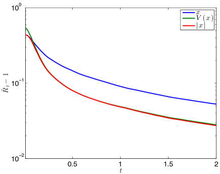
Figure 2. The Gelman-Rubin statistics as a function of time for the observables (4.1) for the Fleming-Viot particle process. The potential is $V(x)=-2\cos(\pi x)$, the state is $(-1,1)$ and the number of replicas is $N=10^{4}$.

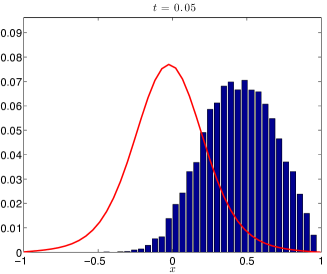
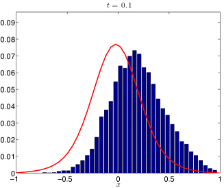
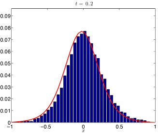
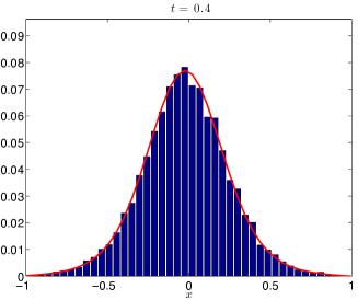
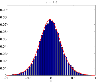
Figure 3. Empirical distributions for the Fleming-Viot particle process on the 1D periodic potential $V(x)=-2\cos(\pi x)$ over the domain $(-1,1)$ with $N=10^{4}$ replicas, see also Figure 2. The red curve is the reference density of the QSD.

4.2. Double Well Potential in 2D

As a second example, we consider the potential

(4.2) $$V(x,y)=\tfrac{1}{6}\left[4(1-x^{2}-y^{2})^{2}+2(x^{2}-2)^{2}+((x+y)^{2}-1)^{2}+((x-y)^{2}-1)^{2}\right],$$

plotted in Figure 4. Notice that there are two minima, near $(\pm 1,0)$, along with an internal barrier, centered at the origin, separating them. Thus, there are two channels joining the two minima, with a saddle point in each of these channels. We study this problem at inverse temperature $\beta=5$. The aim of this example is to illustrate the possibility of pseudo-convergence when using convergence diagnostics, even when it is applied to independent replicas. We thus concentrate on the sampling of the canonical distribution with density $Z^{-1}e^{-\beta V(x,y)}$, using independent realizations, instead of the sampling of the QSD using the Fleming-Viot particle process.

The observables used in this problem are:

(4.3) $$x,\,y,\,V(x,y),\,\left\|{\bf x}\right\|_{\ell^{2}}.$$

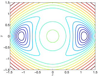
Figure 4. Contours of potential (4.2). Note the two minima, near $(\pm 1,0)$.

Starting our trajectories at $X_{0}=(-1,0)$, the Gelman-Rubin statistics as a function of time appear in Figure 5, and the empirical distributions at two specific times are shown in Figure 6. We make the following remarks.

First, were we to have neglected the $x$ observable, the Gelman-Rubin statistics of the other observables would have fallen below $1.1$ by $t=20$. But as we can see in Figure 6, this is completely inadequate for sampling $Z^{-1}e^{-\beta V(x,y)}$. Thus, if the tolerance is set to $0.1$, the convergence criterion may be fulfilled before actual convergence if the observables are poorly chosen. This is a characteristic problem of convergence diagnostics; they are necessary, but not sufficient to assess convergence.

Let us now consider the $x$ observable, which is sensitive to the internal barrier. From Figure 5, we see that it is not monotonic and that, even after running till $t=2000$, the associated statistic still exceeds $1.1$. On the other hand, if we consider the ensemble at $t=500$, the empirical distribution appears to equally sample both modes. Indeed 48% of the replicas are in the right basin. Despite this, the Gelman-Rubin statistic for $x$ is still relatively large. This is due to the conservative nature of (3.4), already mentioned in Section 4.1. Once the ensemble has an appreciable number of samples in each mode, it will only reach one after all the trajectories have adequately sampled both modes.

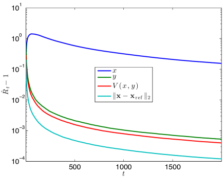
Figure 5. The Gelman-Rubin statistics as a function of time for the observables (4.3) for $N=10^{4}$ independent replicas following the dynamics (2.1). The potential is given by (4.2). Since the replicas begin in the left mode, the internal barrier makes it challenging to adequately sample the $x$ observable.

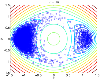
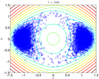
Figure 6. Empirical distributions from $N=10^{4}$ independent replicas following the dynamics (2.1) for the potential (4.2), see also Figure 5.

4.3. Distribution of $t_{\mathrm{corr}}$ and $t_{\mathrm{phase}}$

In the modified ParRep algorithm, $t_{\mathrm{corr}}=t_{\mathrm{phase}}$, determined by (3.5), is a random variable due to $N$ being finite. This introduces some uncertainty in the decorrelation time; it may be that, for a particular realization, (3.5) is satisfied at a time which is too small for the replicas, or the reference process, to have sampled the QSD. This can be mitigated by using more replicas. As $N$ tends to infinity, the empirical distribution of the Fleming-Viot particle process will converge to the law of the process, conditioned on non-extinction, $\mu_{t}$, as in (3.2). Hence, $\hat{R}_{t}(\mathcal{O}_{j})$ tends to a deterministic evolution, and $t_{\mathrm{phase}}$ will approach a deterministic value, for the given observables and tolerance.

To illustrate this, we explored the 1D periodic problem of Section 4.1 with $N=10^{1},10^{2},10^{3},$ and $10^{4}$ replicas at ${\rm TOL}=0.1$. We ran the process until it satisfied (3.5), recording the value of $t_{\mathrm{phase}}$, in each of $10^{4}$ independent realizations, for each of the values of $N$. The results, shown in Figure 7, show the reduction of variability as $N$ becomes large.

In the rest of our examples, appearing in Section 5, we use $N=100$ replicas. The typical variations of $t_{\mathrm{corr}}=t_{\mathrm{phase}}$, measured as the ratio of the standard deviation to the mean of the samples, are 10%–20% of the mean. Both the mean and variance are reported in our data tables, below.

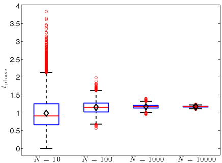
Figure 7. Box plots of $t_{\mathrm{phase}}$ for the 1D periodic problem at different values of $N$ with ${\rm TOL}=0.1$. Each distribution includes $10^{4}$ samples. The box encompasses the middle 50% of the data, the median is the line across the box, and the diamond is the mean. The stems extend out 1.5 times the Interquartile Range (the length of the box). Outliers, outside the stems, are shown with circles.

4.4. Remarks on Numerical Experiments

The problems presented above, though simple, demonstrate both the effectiveness and the caveats of the convergence diagnostics.

First, the convergence diagnostics can be conservative, which is computationally wasteful. Second, there is the possibility of pseudo-convergence: as is the case with all convergence diagnostics, they cannot guarantee stationarity. Thus, some amount of heuristic familiarity with the underlying problem is essential to obtain reasonable results. One should be careful when choosing the observables for (3.4), selecting degrees of freedom which are associated with the metastable features of the dynamics, as revealed by the $x$ observable in the preceding example. Again, the burden is on the practitioner to be familiar with the system and have some sense of the relevant observables to test for stationarity. However, to set, a priori, suitable values of $t_{\mathrm{corr}}$ and $t_{\mathrm{phase}}$ requires more precise knowledge of the system than is needed to apply convergence diagnostics. In some sense, this is comparable to the relationship between a priori and a posteriori estimates in other fields of numerical analysis. a priori estimates are generally insufficient for assessing convergence, since they require some knowledge of the (unknown) solution, such as its regularity. This is why a posteriori estimates have been sought out, to provide error bounds based on computable quantities.

Hence, the reader may wonder why we did not make use of the a priori convergence estimate (2.13) to determine the convergence time to the QSD. The reasons are that we lack estimates of both the exponential rate of convergence, $(\lambda_{2}-\lambda_{1})$, and the prefactor, $C(\mu_{0})$. This is a general challenge to the application of many Markov Chain Monte Carlo algorithms: under very weak assumptions, it can be shown that the law of a Markov Chain converges to equilibrium exponentially fast in time (see, for example, [30]). However, such results cannot be used to estimate the convergence, or burn-in, time since the error bound involves difficult to estimate quantities. The need to identify such a time has motivated the broad investigation of convergence diagnostics for stochastic algorithms.

5. Modified ParRep Examples

In this section we present a number of numerical results obtained with the modified ParRep algorithm. Before presenting the examples, we review the numerical methods and the parameters used in the experiments.

5.1. Common Parameters and Methods

For each problem we compare the direct, serial simulation to our proposed algorithm combining ParRep with the Fleming-Viot particle process and convergence diagnostics, with several different values of ${\rm TOL}$ for the stationarity criterion (3.5). For each case of each problem, we perform $10^{5}$ independent realizations of the experiment to ensure we have adequate data from which to make statistical comparisons. For these ensembles of experiments, which are performed in parallel, SPRNG 2.0, with the linear congruential generator, is used as the pseudo-random number generator, [28]. In all examples, $N=100$ replicas are used.

The stochastic differential equation (2.1) is discretized using Euler-Maruyama with a time step of $\Delta t=10^{-4}$ in all cases except for the experiments in Section 5.4, where, due to the computational complexity, $\Delta t=10^{-3}$. To minimize numerical distortion of the exit times due to the time step discretization, we make use of a correction to time discretized ParRep presented in [2].

Exit distributions obtained from our modified ParRep algorithm and from the direct serial runs are compared using the two sample nonparametric Kolmogorov-Smirnov test (K.-S. Test), [18]. Working at the $\alpha=0.05$ level of significance, this test allows us to determine whether or not we can accept the null hypothesis, which, in this case, is that the samples of exit time distributions arose from the same underlying distribution. Though the test was formulated for continuous distributions, it can also be applied to discrete ones, where it will be conservative with respect to Type 1 statistical errors, [12, 20]. In our tables, we report PASS for instances where the null hypothesis is not rejected (the test cannot distinguish the ParRep results from the direct serial results), and FAIL for cases where the null hypothesis is rejected. We also report the $p$-values, measuring the probability of observing a test statistic at least as extreme as that which is computed.

In the tables below, we also report the mean dephasing time ($\left\langle t_{\mathrm{phase}}\right\rangle$), its variance (${\rm Var}(t_{\mathrm{phase}})$), the average exit time ($\left\langle T\right\rangle$), and the percentage of realizations for which the decorrelation/dephasing step were successful ($\%$ Dephased). The average and variance of $t_{\mathrm{phase}}$ are computed only over realizations for which the reference process decorrelates.

Finally, we report the speedup of the algorithm, which we define as

(5.1) $$\text{Speedup}\equiv\frac{\text{Physical Exit Time}}{\text{Computational Time}}.$$

The computational time is either the exit time of the reference process (if the exit occurs during the decorrelation step), or the sum of the time spent in the decorrelation/dephasing step and in the parallel step (if the exit occurs during the parallel step). Formula (5.1) measures the speedup of the algorithm over direct numerical simulation of the exit event. Let us heuristically consider the mean behavior of (5.1). Let $p$ denote the probability that the system decorrelates, so that $1-p$ corresponds to the probability that the reference process exits before (3.5) is satisfied. For realizations where the reference process exited before decorrelating, the speedup is unity. For realizations which exit in the parallel step, let $\left\langle t_{\mathrm{phase}}\right\rangle$ and $\left\langle t_{\mathrm{par}}\right\rangle$ denote the average dephasing and parallel exit times. Roughly, these values relate to the eigenvalues, introduced in (2.7), and the choice of $N$ as

(5.2) $$\left\langle t_{\mathrm{phase}}\right\rangle\approx\frac{C_{\mathrm{phase}}}{\lambda_{2}-\lambda_{1}},\quad\left\langle t_{\mathrm{par}}\right\rangle\approx\frac{1}{N\lambda_{1}}$$

To obtain $\left\langle t_{\mathrm{par}}\right\rangle$, we have assumed that the dephased distribution is a good approximation of the QSD. The constant $C_{\mathrm{phase}}$ is determined by the initial distribution, the tolerance, the observables, and the temperature of the system.

Thus, assuming these random variables are not too strongly correlated, we have that, roughly,

(5.3) $$\left\langle\text{Speedup}\right\rangle\approx(1-p)+p\frac{\left\langle t_{\mathrm{phase}}\right\rangle+N\left\langle t_{\mathrm{par}}\right\rangle}{\left\langle t_{\mathrm{phase}}\right\rangle+\left\langle t_{\mathrm{par}}\right\rangle}\approx(1-p)+p\frac{\frac{C_{\mathrm{phase}}}{\lambda_{2}-\lambda_{1}}+\frac{1}{\lambda_{1}}}{\frac{C_{\mathrm{phase}}}{\lambda_{2}-\lambda_{1}}+\frac{1}{N\lambda_{1}}}.$$

As $N$ tends to infinity, the maximum speedup monotonically saturates:

(5.4) $$\lim_{N\to\infty}\left\langle\text{Speedup}\right\rangle\approx 1+p\frac{1}{C_{\mathrm{phase}}}\frac{\lambda_{2}-\lambda_{1}}{\lambda_{1}}.$$

Alternatively, if

(5.5) $$N\ll\frac{1}{C_{\mathrm{phase}}}\frac{\lambda_{2}-\lambda_{1}}{\lambda_{1}},$$

we can expand the expression to recover the linear speedup regime,

(5.6) $$\left\langle\text{Speedup}\right\rangle\approx(1-p)+pN\left(1+C_{\mathrm{phase}}\frac{\lambda_{1}}{\lambda_{2}-\lambda_{1}}\right).$$

For strongly metastable systems, we expect that $p$ will be close to one (the reference process almost always decorrelates) and that the relative spectral gap will be large, $\lambda_{2}-\lambda_{1}\gg\lambda_{1}$ (the typical exit time is much larger than the time to converge to the QSD). The constant $C_{\mathrm{phase}}$ will also depend on the degree of metastability, though the dependence is less clear. Thus, we expect there will be a large range of $N$ satisfying (5.5), and a linear speedup will be observed. However, there is also an intrinsic limitation on the performance of ParRep that depends on the strength of metastability of each state.

The ratio in (5.4) has a natural interpretation. As $N$ becomes large in ParRep, the cost of finding the first exit during the parallel step is driven to zero, and what remains is the cost of decorrelation and depahsing. These pieces of the algorithm have a time scale of $(\lambda_{2}-\lambda_{1})^{-1}$. For a direct serial simulation, in a sufficiently metastable system, the cost is to find the first exit, which has a time scale of $\lambda_{1}^{-1}$.

Since dephasing and decorrelation terminate at a finite time, there will always be some bias in the exit distributions, which is in general difficult to distinguish from the statistical noise. When the number of independent realizations of the experiment becomes sufficiently large, the statistical tests may detect this bias and identify two distinct distributions, even if the difference between the two distributions is tiny. Two things are thus to be expected when comparing the exit time distributions obtained by ParRep and direct numerical simulations:

• For a fixed number of independent realizations, as the tolerance is reduced to zero, the $p$-value of the K.-S. test goes to $1$, and the null hypothesis is accepted; the distributions will be the same. This is because, as the tolerance becomes more stringent, it takes longer to reach stationarity. On the one hand, there is then a higher chance that the reference process exits during the joint decorrelation/dephasing step. On the other, for the realizations which manage to satisfy convergence criterion (3.5), the distribution will be closer to that of the QSD. Both these effects induce ParRep to better replicate the true, unaccelerated distributions.

• For fixed tolerance, as the number of realizations tends to $+\infty$, the $p$-value of the K.-S. tends to zero, and the null hypothesis is rejected. This is because as the statistical noise is reduced, the bias due to a finite stationarity time for a given tolerance becomes apparent. This is born out in numerical experiments.

In addition, due to sampling variability, the $p$-value may not vary monotonically as a function of ${\rm TOL}$ or of the number of realizations

5.2. Periodic Potential in 2D

As a first example, we consider the two dimensional periodic potential

(5.7) $$V(x,y)=-\cos(\pi x)-\cos(\pi y),$$

simulated at $\beta=3$. The states are defined as the translates of $(-1,1)^{2}$, seen in Figure 8. The observables used with the Gelman-Rubin statistics in (3.4) are

(5.8) $$x,\quad y,\quad V(x,y),\quad\left\|{\bf x}-{\bf x}_{\mathrm{ref}}\right\|_{\ell^{2}},$$

where ${\bf x}_{\mathrm{ref}}$ will be the local minimum of the state under consideration.

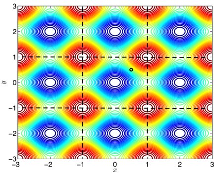
Figure 8. The partition of the configuration space into states for the potential (5.7). The circle $\circ$ indicates the initial condition, $(.5,.5)$.

5.2.1. Escape from a Single State

We first consider the problem of escaping from the state $\Omega=(-1,1)^{2}$ with initial condition $X_{0}=(0.5,0.5)$. We run $10^{5}$ independent realizations of Serial and ParRep simulation, with quantitative data appearing in Table 1, and the distributions in Figures 9.

At the tolerance value ${\rm TOL}=0.2$, there is already good agreement in terms of first hitting point distributions, as seen in Table 5.7. To compare the first hitting point distributions, the boundary of $(-1,1)^{2}$ is treated as a one dimensional manifold composed of the four edges (top, right, bottom, and left); this is the third plot of Figure 9. We indeed have good agreement.

Unlike the exit point distribution, the exit time distribution seems to require a more stringent tolerance. There are statistical errors at ${\rm TOL}=0.2$, which are mitigated as the tolerance is reduced. At ${\rm TOL}=0.05$, the K.-S. test shows agreement. However, based on the first two of Figure 9, the exit time distribution is in good qualitative agreement even for ${\rm TOL}=0.1$, in the sense that the $L^{1}$ distance between the two distributions is small and the decay rates are in agreement.

Notice that for ${\rm TOL}=0.05$, there is good performance in the sense that 84% of the realizations exited during the parallel step, and the statistical agreement is high. The corresponding speedup is 6.25.

With regard to our earlier comment that, at fixed tolerance, as the sample size increases, the $p$-values tend to decrease, we consider the case of ${\rm TOL}=0.1$ here. If we compare the first $10^{2}$, $10^{3}$, $10^{4}$ and $10^{5}$ experimental realizations against the corresponding serial results, we obtain $p$-values of 0.68, 0.18, 0.0099, and 0.0037.

Table 1. Periodic Potential in 2D–Single Escape: Comparison of ParRep and an unaccelerated serial process escaping from $(-1,1)^{2}$ with $X_{0}=(0.5,0.5)$ for potential (5.7).

Method	${\rm TOL}$	$\left\langle t_{\mathrm{phase}}\right\rangle$	${\rm Var}(t_{\mathrm{phase}})$	$\left\langle T\right\rangle$	$\left\langle\text{Speedup}\right\rangle$	% Dephased	$X_{T}$ K.-S. Test ($p$)	$T$ K.-S. Test ($p$)
Serial	–	–	–	34.8	–	–	–	–
ParRep	0.2	1.12	0.0267	35.3	20.8	93.5%	PASS (0.59)	FAIL ($2.0\times 10^{-5}$)
ParRep	0.1	2.43	0.103	35.0	11.6	90.2%	PASS (0.48)	FAIL (0.0037)
ParRep	0.05	5.10	0.393	34.8	6.25	83.6%	PASS (0.52)	PASS (0.33)
ParRep	0.01	26.2	9.08	34.8	1.63	46.5%	PASS (0.27)	PASS (0.42)

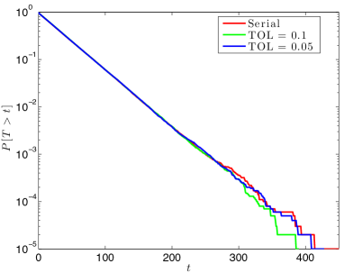
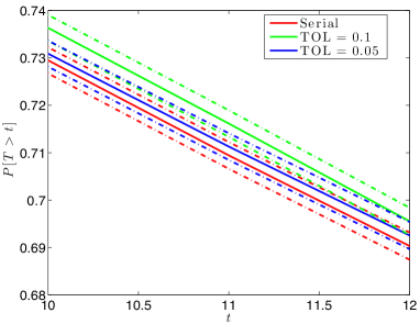
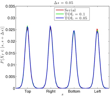
Figure 9. Periodic Potential in 2D–Single Escape: Exit distributions from $\Omega=(-1,1)^{2}$ for the 2D Periodic potential (5.7). On the right is a magnification of the figure from the left; notice that the confidence intervals do not overlap at ${\rm TOL}=.1$. For the hitting point distribution, the boundary of $\Omega$ has been treated as a 1D manifold parametrized clockwise, with the labels “Top”, “Right”, “Bottom”, and “Left” corresponding respectively to the edges $(-1,1)\times\{1\}$, $\{1\}\times(-1,1)$, etc.

5.2.2. Escape from a Region Containing Multiple States

Next, we consider the problem of escaping from the region $(-3,3)^{2}$, running our modified ParRep algorithm over the states indicated in Figure 8. The results are reported in Table 2 and Figure 10. Beneath the value ${\rm TOL}=0.1$, the algorithm is statistically consistent, both in terms of first hitting point and first exit time distributions.

Table 2. Periodic Potential in 2D–Multiple Escapes: Comparison of ParRep and an unaccelerated serial process escaping from $(-3,3)^{2}$ with $X_{0}=(0.5,0.5)$ for potential (5.7).

${\rm TOL}$	$X_{T}$ K.-S. Test ($p$)	$T$ K.-S. Test ($p$)
0.2	PASS (0.56)	FAIL ($5.2\times 10^{-3}$)
0.1	PASS (0.51)	PASS (0.24)
0.05	PASS (0.53)	PASS (0.59)
0.01	PASS (0.11)	PASS (0.87)

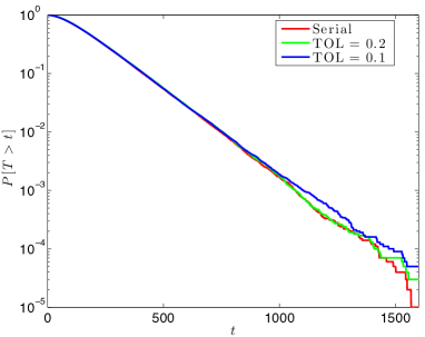
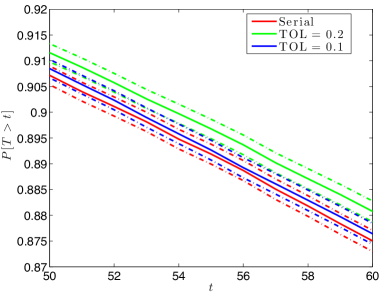
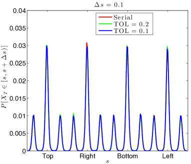
Figure 10. Periodic Potential in 2D–Multiple Escapes: Exit time distribution for the 2D periodic potential (5.7) when ParRep is used to escape from $(-3,3)^{2}$. On the right is a magnification of the figure from the left; notice that the confidence intervals do not overlap at ${\rm TOL}=.2$. For the hitting point distribution, the boundary of $(-3,3)^{2}$ has been treated as a 1D manifold parametrized clockwise, with the labels “Top”, “Right”, “Bottom”, and “Left” corresponding respectively to the edges $(-3,3)\times\{3\}$, $\{3\}\times(-3,3)$, etc.

5.3. Entropic Barriers in 2D

Let us now consider a test case with entropic barriers. Consider pure Brownian motion in the domain represented in Figure 11, with reflecting boundary conditions. Here, the observables are

(5.9) $$x,\,y,\,\left\|{\bf x}-{\bf x}_{\mathrm{ref}}\right\|_{\ell^{2}},$$

with the reference points indicated in Figure 11.

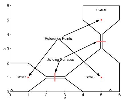
Figure 11. A domain with entropic barriers. The trajectory begins at $(5.5,0.1)$ for the experiment in Section 5.3.1 and at $(0.1,0.1)$ for the experiment in Section 5.3.2 (see the $\circ$ symbols). The width of the necks between states is 0.1, and the dividing surfaces between states are indicated by the short segments. A separate reference point is used in each state for the observable $\left\|{\bf x}-{\bf x}_{\mathrm{ref}}\right\|$.

5.3.1. Escape from State 2

As a first experiment, we look for first escapes from state 2, with initial condition $(5.5,0.1)$. Quantitative results appear in Table 3 and the exit time distributions are plotted in Figure 12. For this problem, there is good statistical agreement even at ${\rm TOL}=0.2$. As the hitting point distributions across each of the two channels are nearly uniform, we only report the probability of passing into state 3 versus state 1. Note that in the ${\rm TOL}=0.01$ case, the exit is almost always due to the reference process escaping before stationarity is achieved. This is an example of setting the parameter so stringently as to render ParRep inefficient.

Table 3. Entropic Barrier in 2D–Single Escape: Comparison of ParRep and an unaccelerated serial process escaping from state 2 of Figure 11 with initial condition $(5.5,.1)$.

Method	${\rm TOL}$	$\left\langle t_{\mathrm{phase}}\right\rangle$	${\rm Var}(t_{\mathrm{phase}})$	$\left\langle T\right\rangle$	$\left\langle\text{Speedup}\right\rangle$	% Dephased	$\mathbb{P}[\text{state 3}]$	$T$ K.-S. Test ($p$)
Serial	–	–	–	45.0	–	–	$(0.493,0.500)$	–
ParRep	0.2	12.7	2.31	44.8	3.46	77.9%	$(0.495,0.502)$	PASS (0.90)
ParRep	0.1	25.4	8.75	45.1	1.95	58.0%	$(0.493,0.499)$	PASS (0.51)
ParRep	0.05	50.3	33.3	45.1	1.27	32.3%	$(0.497,0.503)$	PASS (0.41)
ParRep	0.01	236.0	658.0	45.1	1.00	0.342%	$(0.496,0.502)$	PASS (0.31)

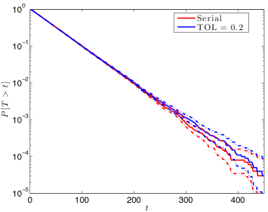
Figure 12. Entropic Barrier in 2D–Single Escape: Exit time distribution from state 2 of Figure 11 with initial conditions $(5.5,.1)$, along with confidence intervals.

5.3.2. Getting to State 3 from State 1

As a second experiment, we start the trajectories in state 1 at $(0.1,0.1)$, and examine how long it takes to get to state 3, running the modified ParRep algorithm over the states represented on Figure 11. The results of this experiment are given in Table 4 and Figure 13. Again, there is a very good statistical agreement in all cases.

Table 4. Entropic Barrier in 2D–Multiple Escapes: Comparison of ParRep and an unaccelerated serial process getting from state 1 to state 3 with initial condition $(.1,.1)$; see Figure 11.

${\rm TOL}$	$T$ K.-S. Test ($p$)
0.2	PASS (0.070)
0.1	PASS (0.14)
0.05	PASS (0.090)
0.01	PASS (0.74)

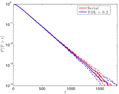
Figure 13. Entropic Barrier in 2D–Multiple Escapes: Exit time distributions to get to state 3 from state 1 in the entropic barrier problem pictured in Figure 11, along with confidence intervals. The full algorithm is applied in each state the trajectory visits.

5.4. Lennard-Jones Clusters

For a more realistic problem, we consider a Lennard-Jones cluster of seven atoms in 2D, denoted ${\rm LJ}_{7}^{{\rm 2D}}$. The potential used in this problem is then:

(5.10) $$V_{7}^{\rm 2D}({\bf x})=\frac{1}{2}\sum_{i\neq j}\phi(\left\|{\bf x}_{i}-{\bf x}_{j}\right\|),\quad{\bf x}=({\bf x}_{1},{\bf x}_{2},\ldots,{\bf x}_{7}),\quad\phi(r)=r^{-12}-2r^{-6}.$$

Due to the computational cost associated with this problem, the time step size is increased to $\Delta t=10^{-3}$. A smaller time step could have been used, but we would have been precluded from obtaining large samples of the problem.

The initial condition in this problem is near the closest packed configuration, with six atoms located $\pi/3$ radians apart on a unit circle and one in the center, as shown in Figure 14 (a). We then look at first exits from this configuration at inverse temperature $\beta=6$. Exits correspond to transitions into basins of attraction for a conformation other than the lowest energy, closest packed, conformation; see Figure 14. Here, basins of attraction are those associated to the simple gradient dynamics $\dot{x}=-\nabla V(x)$: these basins define the states on which ParRep is applied. For the numbering of the conformations, we adopt the notation found in [14], where the authors also explore transitions in ${\rm LJ}_{7}^{{\rm 2D}}$. We also refer to [19] for an algorithm for computing transitions within Lennard-Jones clusters.

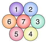
(a) $C_{0}$, $V=-12.53$

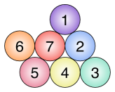
(b) $C_{1}$, $V=-11.50$

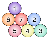
(c) $C_{2}$, $V=-11.48$

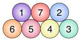
(d) $C_{3}$, $V=-11.40$

Figure 14. Low energy conformations of the Lennard-Jones cluster of seven atoms in 2D. Also indicated are the associated energy levels.

Before proceeding to our results, we make note of several things that are specific to this problem. States are identified and compared as follows:

1. Given the current configuration $X_{t}$, a gradient descent is run (following the dynamics $\dot{x}=-\nabla V(x)$ with $x_{0}=X_{t}$) until the norm of the gradient becomes sufficiently small. This is accomplished using the RK45 time discretization scheme, up to the time when the $\ell^{2}$ norm of the gradient, relative to the value of $\left|V\right|$, is smaller than $10^{-5}$;

2. Once the local minima is found, in order to identify the conformation, the lengths of the twenty one “bonds” between pairs of atoms are computed. Let $b_{ij}$ denote the distance between the atoms $i$ and $j$.

3. The current and previous states are compared using the $\ell^{1}$ norm between the 21 bond lengths:

   $$\text{Distance to $C_{0}$}=\sum_{1\leq i<j\leq 7}\left|b_{ij}-b_{ij}^{0}\right|$$

   where $b_{ij}^{0}$ are the bond lengths of the $C_{0}$ conformation.

4. If this distance exceeds .5, the states are determined to be different.

Next, when examining the output, we group conformations according to energy levels. In Figure 14, we present for each conformation $C_{0}$, $C_{1}$, $C_{2}$ and $C_{3}$ a particular numbering. Other permutations of the atoms also correspond to the same energy level, and thus to the same conformation.

The observables that are used in this problem are:

(5.11a) Energy: $$V(x)$$

(5.11b) Square distance to the center of mass: $$\sum_{i=1}^{7}\left\|x_{i}-x_{\rm cm}\right\|_{\ell^{2}}^{2}$$

(5.11c) Distance to $$C_{0} \sum_{1\leq i<j\leq 7}\left|b_{ij}-b_{ij}^{0}\right|$$:

It is essential to use observables that are rotation and translation invariant, as there is nothing to prevent the cluster from drifting or rotating (i.e. no atom is pinned).

A related remark is that, to not introduce additional auxiliary parameters, no confining potential is used. Because of this, the cluster does not always change into one of the other conformations. In some cases, an atom can drift away from the cluster, and the quenched configuration corresponds to the isolated atom and the five remaning atoms. In others, the quenched configuration corresponds to $C_{0}$, but with two exterior atoms exchanged. These scenarios occurred in less than .1% of the $10^{5}$ realizations of all experiments, both ParRep and unaccelerated.

Over 99.9% of the transitions from $C_{0}$ are to $C_{1}$ or $C_{2}$. A transition from $C_{0}$ to $C_{3}$ has not been observed. Since there are thus only two ways to leave $C_{0}$, we use the 95% Clopper-Pearson confidence intervals [21] (well adapted to binomial random variables) to assess the quality of the exit point distribution in our statistical tests.

Our statistical assessment of ParRep is given in Tables 5 and 6. It is only at the most stringent tolerance of ${\rm TOL}=0.01$ that an excellent agreement is obtained in the exit time distribution, though some amount of speedup is still gained. As in the other problems, the Kolmogorov-Smirnov test may be an overly conservative measure of the quality of ParRep. As shown in Figure 15, the exit time distributions are already in good qualitative agreement, even at less stringent tolerances. In contrast, the transition probabilities to the other conformations are in very good agreement at tolerances beneath 0.1.

Table 5. ${\rm LJ}_{7}^{{\rm 2D}}$-Single Escape: Comparison of the exit times for ParRep and an unaccelerated serial process escaping from the closest packed ${\rm LJ}_{7}^{{\rm 2D}}$ configuration.

Method	${\rm TOL}$	$\left\langle t_{\mathrm{phase}}\right\rangle$	${\rm Var}(t_{\mathrm{phase}})$	$\left\langle T\right\rangle$	$\left\langle\text{Speedup}\right\rangle$	% Dephased	$T$ K.-S. Test ($p$)
Serial	–	–	–	17.0	–	–	–
ParRep	0.2	0.411	0.0336	19.1	29.3	98.5%	FAIL ($3.6\times 10^{-235}$)
ParRep	0.1	.976	0.125	18.0	14.9	95.3%	FAIL ($5.0\times 10^{-55}$)
ParRep	0.05	2.08	0.433	17.6	7.83	90.0%	FAIL ($9.4\times 10^{-28}$)
ParRep	0.01	10.8	5.67	17.0	1.82	52.1%	PASS (0.92)

Table 6. ${\rm LJ}_{7}^{{\rm 2D}}$-Single Escape: Comparison of the hitting points for ParRep and an unaccelerated serial process escaping from the closest packed ${\rm LJ}_{7}^{{\rm 2D}}$ configuration.

Method	${\rm TOL}$	$\mathbb{P}[C_{1}]$	$\mathbb{P}[C_{2}]$
Serial	–	(0.502, 0.508)	(0.491, 0.498)
ParRep	0.2	(0.508, 0.514)	(0.485, 0.492)
ParRep	0.1	(0.506, 0.512)	(0.488, 0.494)
ParRep	0.05	(0.505, 0.512)	(0.488, 0.495)
ParRep	0.01	(0.504, 0.510)	(0.490, 0.496)

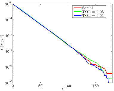
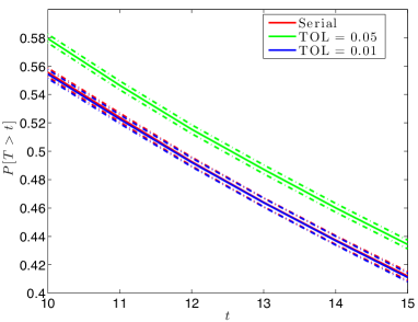
Figure 15. ${\rm LJ}_{7}^{{\rm 2D}}$-Single Escape: Exit time distributions for ${\rm LJ}_{7}^{{\rm 2D}}$ at $\beta=6$.

5.5. Conclusions from the Numerical Experiments

From these numerical experiments, we observe that the modified ParRep is indeed an efficient algorithm on various test cases, for which no a priori knowledge on the decorrelation/dephasing time has been used. We thus trade setting $t_{\mathrm{corr}}$ and $t_{\mathrm{phase}}$, a priori, for selecting physically informed observables together with a tolerance. In conclusion, a tolerance on the order of 0.1 in (3.4) seems to yield sensible results.

We also observe that the tolerance criteria used to assess stationarity does not need to be very stringent to get the correct distribution for the hitting points (thus to get the correct state-to-state Markov chains). In contrast, the K.-S. test on the exit time distribution requires smaller tolerances to predict statistical agreement. However, even when the K.-S. test fails to reject the null hypothesis, the agreement is very good. Overall, it is easier to obtain statistical agreement in the sequence of visited states than it is to get statistical agreement of the time spent within each state.

References

- [1] D. Aristoff and T. Lelièvre. Mathematical Analysis of Temperature Accelerated Dynamics. MMS, 12(1):290–317, 2014.
- [2] D. Aristoff, T. Lelièvre, and G. Simpson. The parallel replica method for simulating long trajectories of Markov chains. Appl. Math. Res. Express, 2014:332–352, 2014.
- [3] S. Asmussen and P. W. Glynn. Stochastic Simulation: Algorithms and Analysis. Springer, November 2010.
- [4] S. Brooks, A. Gelman, G. Jones, and X.-L. Meng. Handbook of Markov Chain Monte Carlo. Chapman and Hall/CRC, 2011.
- [5] S.P. Brooks and A. Gelman. General methods for monitoring convergence of iterative simulations. J. Comput. Graph. Stat., pages 434–455, 1998.
- [6] SP Brooks and GO Roberts. Convergence assessment techniques for Markov chain Monte Carlo. Stat. Comp., 8(4):319–335, 1998.
- [7] P. Cattiaux, P. Collet, A. Lambert, S. Martínez, S. Méléard, and J. San Martín. Quasi-stationary distributions and diffusion models in population dynamics. Ann. Probab., 37(5):1926–1969, 2009.
- [8] P. Cattiaux and S. Méléard. Competitive or weak cooperative stochastic Lotka-Volterra systems conditioned on non-extinction. J. Math. Biol., 60(6):797–829, 2010.
- [9] P. Collet, S. Martínez, and J. San Martín. Asymptotic laws for one-dimensional diffusions conditioned to nonabsorption. Ann. Probab., 23(3):1300–1314, 1995.
- [10] P. Collet, S. Martinez, and J. San Martin. Quasi-Stationary Distributions. Springer, 2013.
- [11] Mary Kathryn Cowles and Bradley P. Carlin. Markov chain Monte Carlo convergence diagnostics: a comparative review. J. Amer. Statist. Assoc., 91(434):883–904, 1996.
- [12] H. L. Crutcher. A note on the possible misuse of the Kolmogorov-Smirnov test. J. Appl. Meteorol., 14(8):1600–1603, 1975.
- [13] P. Del Moral. Feynman-Kac Formulae. Springer, 2004.
- [14] C Dellago, P G Bolhuis, and D Chandler. Efficient transition path sampling: Application to Lennard-Jones cluster rearrangements. J. Chem. Phys., 108(22):9236–9245, 1998.
- [15] P.A. Ferrari and N. Maric. Quasi stationary distributions and Fleming-Viot processes in countable spaces. Electron. J. Probab., 12(24):684–702, 2007.
- [16] M. Galassi, J. Davies, J. Theiler, B. Gough, G. Jungman, P. Alken, M. Booth, and F. Rossi. GNU Scientific Library, March 2013.
- [17] A. Gelman and D.B. Rubin. Inference from iterative simulation using multiple sequences. Stat. Sci., 7(4):457–472, 1992.
- [18] J. D. Gibbons. Nonparametric Methods for Quantitative Analysis. American Sciences Press, Third edition, 1997.
- [19] M. Hairer and J. Weare. Improved diffusion Monte Carlo and the Brownian fan. arXiv:1207.2866, 2012.
- [20] S. D. Horn. Goodness-of-fit tests for discrete data: a review and an application to a health impairment scale. Biometrics, 33(1):237, 1977.
- [21] N. L. Johnson, A. W. Kemp, and S. Kotz. Univariate discrete distributions. Wiley, Third edition, 2005.
- [22] S. Kirmizialtin and R. Elber. Revisiting and computing reaction coordinates with directional milestoning. J. Phys. Chem. A, 115(23):6137–6148, 2011.
- [23] O. Kum, B. M. Dickson, S. J. Stuart, B. P. Uberuaga, and A. F. Voter. Parallel replica dynamics with a heterogeneous distribution of barriers: Application to n-hexadecane pyrolysis. The Journal of Chemical Physics, 121(20):9808, 2004.
- [24] C. Le Bris, T. Lelièvre, M. Luskin, and D. Perez. A mathematical formalization of the parallel replica dynamics. Monte Carlo Meth. Appl., 18(2):119–146, 2012.
- [25] T. Lelièvre and F. Nier. Low temperature asymptotics for quasi-stationary distribution in a bounded domain. arXiv:1309.3898, 2013.
- [26] S. Martínez and J. San Martín. Quasi-stationary distributions for a Brownian motion with drift and associated limit laws. J. Appl. Probab., 31(4):911–920, 1994.
- [27] S. Martínez and J. San Martín. Classification of killed one-dimensional diffusions. Ann. Probab., 32(1A):530–552, 2004.
- [28] M. Mascagni and A. Srinivasan. Algorithm 806: SPRNG: a scalable library for pseudorandom number generation. TOMS, 26(3), September 2000.
- [29] S. Méléard and D. Villemonais. Quasi-stationary distributions and population processes. Probability Surveys, 2012.
- [30] S. Meyn and R. L. Tweedie. Markov Chains and Stochastic Stability. Cambridge University Press, second edition, 2009.
- [31] D. Perez, B.P. Uberuaga, Y. Shim, J.G. Amar, and A.F. Voter. Accelerated molecular dynamics methods: introduction and recent developments. Ann. Rep. Comp. Chem., 5:79–98, 2009.
- [32] G. Simpson and M. Luskin. Numerical analysis of parallel replica dynamics. M2AN, 47(5):1287–1314, 2013.
- [33] M. R. Sørensen and A. F. Voter. Temperature-accelerated dynamics for simulation of infrequent events. J. Chem. Phys., 112(21):9599–9606, 2000.
- [34] D. Steinsaltz and S. N. Evans. Quasistationary distributions for one-dimensional diffusions with killing. T. Am. Math. Soc., 359(3):1285–1324 (electronic), 2007.
- [35] A.-S. Sznitman. Topics in propagation of chaos. In École d’Été de Probabilités de Saint-Flour XIX—1989, volume 1464 of Lecture Notes in Math., pages 165–251. Springer, 1991.
- [36] E. Vanden-Eijnden, M. Venturoli, G. Ciccotti, and R. Elber. On the assumptions underlying milestoning. J. Chem. Phys., 129(17):174102, 2008.
- [37] A.F Voter. Hyperdynamics: Accelerated molecular dynamics of infrequent events. Phys. Rev. Lett., 78(20):3908–3911, 1997.
- [38] A.F Voter. A method for accelerating the molecular dynamics simulation of infrequent events. J. Chem. Phys., 106(11):4665–4677, 1997.
- [39] A.F. Voter. Parallel replica method for dynamics of infrequent events. Phys. Rev. B, 57(22):13985–13988, 1998.
- [40] A.F. Voter, F. Montalenti, and T.C. Germann. Extending the time scale in atomistic simulation of materials. Ann. Rev. Mater. Sci, 32:321–346, 2002.