Ensemble estimation of multivariate $f$-divergence

Abstract

$f$-divergence estimation is an important problem in the fields of information theory, machine learning, and statistics. While several divergence estimators exist, relatively few of their convergence rates are known. We derive the MSE convergence rate for a density plug-in estimator of $f$-divergence. Then by applying the theory of optimally weighted ensemble estimation, we derive a divergence estimator with a convergence rate of $O\left(\frac{1}{T}\right)$ that is simple to implement and performs well in high dimensions. We validate our theoretical results with experiments.

I Introduction

$f$-divergence is a measure of the difference between distributions and is important to the fields of information theory, machine learning, and statistics [1]. Many different kinds of $f$-divergences have been defined including the Kullback-Leibler (KL) [2] and Rényi-$\alpha$ [3]. A special case of the KL divergence is mutual information which gives the capacities in data compression and channel coding [4]. Mutual information estimation has also been used in applications such as feature selection [5], fMRI data processing [6], and clustering [7]. Entropy is also a special case of divergence where one of the distributions is the uniform distribution. Entropy estimation is useful for intrinsic dimension estimation [8], texture classification and image registration [9], and many other applications. Additionally, divergence estimation is useful for empirically estimating the decay rates of error probabilities of hypothesis testing [4] and extending machine learning algorithms to distributional features [10, 11]. For other applications of divergence estimation, see [12].

We consider the problem of estimating the $f$-divergence when only two finite populations of independent and identically distributed (i.i.d.) samples are available from some unknown, nonparametric, smooth, $d$-dimensional distributions. While several estimators of divergence have been previously defined, the convergence rates are known for only a few of them. Our first contribution is to derive convergence rates for kernel density plug-in $f$-divergence estimators with an adaptive $k$-nearest neighbor ($k$-nn) kernel. Our second contribution is to extend the theory of optimally weighted ensemble entropy estimation developed in [13] to obtain a divergence estimator with a convergence rate of $O\left(\frac{1}{T}\right)$ where $T$ is the sample size. This is accomplished by solving an offline convex optimization problem.

I-A Related Work

Several estimators for some $f$-divergences already exist. For example, Póczos & Schneider [10] established weak consistency of a bias-corrected $k$-nn estimator for Rényi-$\alpha$ and other divergences of similar form. Wang et al [12] gave an estimator for the KL divergence. Other mutual information and divergence estimators based on plug-in histogram schemes have been proven to be consistent [14, 15, 16, 17]. However none of these works studied the convergence rates of their estimators while our ensemble approach requires an explicit expression of the asymptotic bias and variance. Hero et al [9] provided an estimator for Rényi-$\alpha$ divergence but assumed that one of the densities was known.

Nguyen et al [18] proposed a method for estimating $f$-divergences by estimating the likelihood ratio of the two densities by solving a convex optimization problem and then plugging it into the divergence formulas. For this method they prove that the minimax convergence rate is parametric ($O\left(\frac{1}{T}\right)$) when the likelihood ratio is in the bounded Hölder class $\Sigma_{\kappa}(\beta,L,r)$ with $\beta\geq d/2$. This assumption is weaker than ours which requires the densities to be at least $d$ times differentiable. However, solving the convex problem of [18] is similar in complexity to training the SVM (between $O(T^{2})$ and $O(T^{3})$) which can be demanding when $T$ is very large. In contrast, our method of optimally weighted ensemble estimation depends only on simple density plug-in estimates and an offline convex optimization problem. Thus the most computationally demanding step in our approach is the calculation of the $k$-nn distances which has complexity no greater than $O(T^{2})$.

Singh and Póczos [19] provided an estimator for Rényi-$\alpha$ divergences that uses a “mirror image” kernel density estimator. They prove a convergence rate of $O\left(\frac{1}{T}\right)$ when $\beta\geq d$ for each of the densities. However this method requires several computations at each boundary of the support of the densities which becomes difficult to implement as $d$ gets large. Also, this method requires knowledge of the support of the densities which may not be possible for some problems.

The main results of our paper are as follows. First, under the assumption that the densities are smooth, lower bounded, and have bounded support, the mean squared error (MSE) of a kernel density plug-in estimator of $f$-divergence converges to zero at the non-parametric rate of $O\left(T^{-1/d}\right),$ which becomes exceedingly slow as dimension $d$ increases. Second, the proposed weighted ensemble estimator of divergence is simple to implement and its MSE converges at the parametric rate of $O\left(\frac{1}{T}\right)$. Third, the proposed estimator of divergence is shown by simulation to outperform standard kernel density plug-in estimators for modest sample sizes ($T\geq 400$) and in high dimensions ($d\geq 4$). Finally, the proposed divergence estimator performs well even for densities with unbounded support (Gaussian), suggesting that our theory holds under significantly weaker assumptions.

I-B Organization and Notation

The paper is organized as follows. Section II provides the theory underlying the optimally weighted ensemble estimator. Section III applies this theory to $f$-divergence estimation and gives convergence results for the estimators, while Section III-C provides proofs. Section IV gives some experimental results that illustrate the performance of our estimators as a function of $T$ and $d$. Section V concludes the paper.

Bold face type is used for random variables and random vectors. Let $f_{1}$ and $f_{2}$ be densities and define $L(x)=\frac{f_{1}(x)}{f_{2}(x)}$. The conditional expectation given a random variable $\mathbf{Z}$ is denoted $\mathbb{E}_{\mathbf{Z}}$. The variance of a random variable is denoted $\mathbb{V}$ and the bias of an estimator is denoted $\mathbb{B}$.

II Weighted ensemble estimation

Let $\bar{l}=\left\{l_{1},\dots,l_{L}\right\}$ be a set of index values and $T$ the number of samples available. For an indexed ensemble of estimators $\left\{\hat{\mathbf{E}}_{l}\right\}_{l\in\bar{l}}$ of the parameter $E$, the weighted ensemble estimator with weights $w=\left\{w\left(l_{1}\right),\dots,w\left(l_{L}\right)\right\}$ satisfying $\sum_{l\in\bar{l}}w(l)=1$ is defined as

$$\hat{\mathbf{E}}_{w}=\sum_{l\in\bar{l}}w\left(l\right)\hat{\mathbf{E}}_{l}.$$

$\hat{\mathbf{E}}_{w}$ is asyptotically unbiased if the estimators $\left\{\hat{\mathbf{E}}_{l}\right\}_{l\in\bar{l}}$ are asymptotically unbiased. Typically the MSE of a plug-in estimator is dominated by the bias. The key idea to reducing MSE is that by choosing appropriate weights $w$, we can greatly decrease the bias in exchange for some increase in variance. Suppose the following conditions are satisfied by $\left\{\hat{\mathbf{E}}_{l}\right\}_{l\in\bar{l}}$ [13]:

• $\mathcal{C}.1$ The bias is given by

  $$\mathbb{B}\left(\hat{\mathbf{E}}_{l}\right)=\sum_{i\in J}c_{i}\psi_{i}(l)T^{-i/2d}+O\left(\frac{1}{\sqrt{T}}\right),$$

  where $c_{i}$ are constants depending on the underlying density, $J=\left\{i_{1},\dots,i_{I}\right\}$ is a finite index set with $I<L$, $\min(J)>0$ and $\max(J)\leq d$, and $\psi_{i}(l)$ are basis functions depending only on the parameter $l$.

• $\mathcal{C}.2$ The variance is given by

  $$\mathbb{V}\left[\hat{\mathbf{E}}_{l}\right]=c_{v}\left(\frac{1}{T}\right)+o\left(\frac{1}{T}\right).$$

Theorem 1.

[13] Assume conditions $\mathcal{C}.1$ and $\mathcal{C}.2$ hold for an ensemble of estimators $\left\{\hat{\mathbf{E}}_{l}\right\}_{l\in\bar{l}}$. Then there exists a weight vector $w_{0}$ such that

$$\mathbb{E}\left[\left(\hat{\mathbf{E}}_{w_{0}}-E\right)^{2}\right]=O\left(\frac{1}{T}\right).$$

The weight vector $w_{0}$ is the solution to the following convex optimization problem:

$$\begin{array}[]{rl}\min_{w}&||w||_{2}\\ subject\,to&\sum_{l\in\bar{l}}w(l)=1,\\ &\gamma_{w}(i)=\sum_{l\in\bar{l}}w(l)\psi_{i}(l)=0,\,i\in J.\end{array}$$

III Application to divergence estimation

Theorem 1 was applied in [13] to obtain an entropy estimator with parametric convergence rates $O\left(\frac{1}{T}\right).$ An analogous theorem will be presented that applies ensemble estimation of estimators of $f$-divergence. Specifically, we focus on divergences that include the form [1]

$$G(f_{1},f_{2})=\int g\left(\frac{f_{1}(x)}{f_{2}(x)}\right)f_{2}(x)dx,$$ (1)

for some smooth, convex function $g(f)$. Divergences that have this form include the Renyi divergence ($g(x)=x^{\alpha}$) and the KL divergence ($g(x)=-\ln x$). We assume that the $d$-dimensional multivariate densities $f_{1}$ and $f_{2}$ have finite support $\mathcal{S}=\left[a,b\right]^{d}$. Assume that $T=N+M_{2}$ i.i.d. realizations $\left\{\mathbf{X}_{1},\dots,\mathbf{X}_{N},\mathbf{X}_{N+1},\dots,\mathbf{X}_{N+M_{2}}\right\}$ are available from the density $f_{2}$ and $M_{1}$ i.i.d. realizations $\left\{\mathbf{Y}_{1},\dots,\mathbf{Y}_{M_{1}}\right\}$ are available from the density $f_{1}$.

We use $k$-nn density estimators in our proposed $f$-divergence estimator. Assume that $k_{i}\leq M_{i}.$ Let $\rho_{2,k_{2}}(i)$ be the distance of the $k_{2}$th nearest neighbor of $X_{i}$ in $\left\{X_{N+1},\dots,X_{T}\right\}$ and let $\rho_{1,k_{1}}(i)$ be the distance of the $k_{1}$th nearest neighbor of $X_{i}$ in $\left\{Y_{1},\dots,Y_{M_{1}}\right\}.$ Then the $k$-nn density estimate is [20]

$$\hat{\mathbf{f}}_{i,k_{i}}(X_{j})=\frac{k_{i}}{M_{i}\bar{c}\mathbf{\mathbf{\rho}}_{i,k_{i}}^{d}(j)},$$

where $\bar{c}$ is the volume of a $d$-dimensional unit ball.

The plug-in estimator of divergence is constructed similarly to [13]. The data from $f_{2}$ are randomly divided into two parts $\left\{\mathbf{X}_{1},\dots,\mathbf{X}_{N}\right\}$ and $\left\{\mathbf{X}_{N+1},\dots,\mathbf{X}_{N+M_{2}}\right\}$. The density estimate $\hat{\mathbf{f}}_{2,k_{2}}$ is found at the $N$ points $\left\{\mathbf{X}_{1},\dots,\mathbf{X}_{N}\right\}$ using the $M_{2}$ realizations $\left\{\mathbf{X}_{N+1},\dots,\mathbf{X}_{N+M_{2}}\right\}$. Splitting the data in this manner is a common approach to debiasing and variance reduction in non-parametric estimation. Similarly, the density estimate $\hat{\mathbf{f}}_{1,k_{1}}$ is found at the $N$ points $\left\{\mathbf{X}_{1},\dots,\mathbf{X}_{N}\right\}$ using the $M_{1}$ realizations $\left\{\mathbf{Y}_{1},\dots,\mathbf{Y}_{M_{1}}\right\}$. Define $\hat{\mathbf{L}}_{k_{1},k_{2}}(x)=\frac{\hat{\mathbf{f}}_{1,k_{1}}(x)}{\hat{\mathbf{f}}_{2,k_{2}}(x)}.$ The functional $G(f_{1},f_{2})$ is then approximated as

$$\hat{\mathbf{G}}_{k_{1},k_{2}}=\frac{1}{N}\sum_{i=1}^{N}g\left(\hat{\mathbf{L}}_{k_{1},k_{2}}\left(\mathbf{X}_{i}\right)\right).$$ (2)

This is a plug-in estimator in the sense that we plug in the estimates to the argument of the expectation, and then use the empirical average to calculate the expectation.

Similar to [13], the principal assumptions we make on the densities $f_{1}$ and $f_{2}$ and the functional $g$ are that: 1) $f_{1}$, $f_{2},$ and $g$ are smooth; 2) $f_{1}$ and $f_{2}$ have common bounded support sets $\mathcal{S}$; 3) $f_{1}$ and $f_{2}$ are strictly lower bounded. Specifically:

• $(\mathcal{A}.0)$: Assume that $k_{i}=k_{0}M_{i}^{\beta}$ with $0<\beta<1$, that $M_{2}=\alpha_{frac}T$ with $0<\alpha_{frac}<1$.

• $(\mathcal{A}.1)$: Assume there exist constants $\epsilon_{0},\epsilon_{\infty}$ such that $0<\epsilon_{0}\leq f_{i}(x)\leq\epsilon_{\infty}<\infty,\,\forall x\in S.$

• $(\mathcal{A}.2)$: Assume that the densities $f_{i}$ have continuous partial derivatives of order $d$ in the interior of $\mathcal{S}$ that are upper bounded.

• $(\mathcal{A}.3)$: Assume that $g$ has derivatives $g^{(j)}$ of order $j=1,\dots,\max\{\lambda,d\}$ where $\lambda\beta>1$.

• $(\mathcal{A}.4$): Assume that $\left|g^{(j)}\left(f_{1}(x)/f_{2}(x)\right)\right|$, $j=0,\ldots,\max\{\lambda,d\}$ are strictly upper bounded for $\epsilon_{0}\leq f_{i}(x)\leq\epsilon_{\infty}.$

• $(\mathcal{A}.5)$: Let $\epsilon\in(0,1)$, $\delta\in(2/3,1)$, and $\mathcal{C}(k)=\exp\left(-3k^{(1-\delta)}\right).$ For fixed $\epsilon,$ define $p_{l,i}=(1-\epsilon)\epsilon_{0}\frac{k_{i}-1}{M_{i}}$, $p_{u,i}=(1+\epsilon)\epsilon_{\infty}\frac{k_{i}-1}{M_{i}}$, $q_{l,i}=\frac{k_{i}-1}{M_{i}\bar{c}D^{d}},$ and $q_{u,i}=(1+\epsilon)\epsilon_{\infty}$ where $D$ is the diameter of the support $S.$ Let $\mathbf{P}_{i}$ be a beta distributed random variable with parameters $k_{i}$ and $M_{i}-k_{i}+1.$ Define $p_{l}=\frac{p_{l,1}}{p_{u,2}}$ and $p_{u}=\frac{p_{u,1}}{p_{l,2}}$. Assume that for $U(L)=g(L),\,g^{(3)}(L),$ and $g^{(\lambda)}(L),$

  • $(i)\,\mathbb{E}\left[\sup_{L\in(p_{l},p_{u})}\left|U\left(L\frac{\mathbf{P}_{2}}{\mathbf{P}_{1}}\right)\right|\right]=G_{1}<\infty$,

  • $(ii)\,\sup_{L\in\left(\frac{q_{l,1}}{q_{u,2}},\frac{q_{u,1}}{q_{l,2}}\right)}\left|U\left(L\right)\right|\mathcal{C}\left(k_{1}\right)\mathcal{C}\left(k_{2}\right)=G_{2}<\infty,$

  • $(iii)\,\mathbb{E}\left[\sup_{L\in\left(\frac{q_{l,1}}{p_{u,2}},\frac{q_{u,1}}{p_{l,2}}\right)}\left|U\left(L\mathbf{P}_{2}\right)\right|\mathcal{C}\left(k_{1}\right)\right]=G_{3}<\infty,$

  • $(iv)\,\mathbb{E}\left[\sup_{L\in\left(\frac{p_{l,1}}{q_{u,2}},\frac{p_{u,1}}{q_{l,2}}\right)}\left|U\left(\frac{L}{\mathbf{P}_{1}}\right)\right|\mathcal{C}\left(k_{2}\right)\right]=G_{4}<\infty,\,\forall M_{i}.$

Densities for which assumptions $\mathcal{A}.0-\mathcal{A}.5$ hold include the truncated Gaussian distribution and the Beta distribution on the unit cube. Functions for which the assumptions hold include $g(L)=-\ln L$ and $g(L)=L^{\alpha}.$

III-A Analysis of mean squared error

The following hold under assumptions $\mathcal{A}.0-\mathcal{A}.5$:

Theorem 2.

The bias of the plug-in estimator $\hat{\mathbf{G}}_{k_{1},k_{2}}$ is given by

$$\mathbb{B}\left(\hat{\mathbf{G}}_{k_{1},k_{2}}\right)=\sum_{j=1}^{d}\left(c_{6,j,1}\left(\frac{k_{1}}{M_{1}}\right)^{\frac{j}{d}}+c_{6,j,2}\left(\frac{k_{2}}{M_{2}}\right)^{\frac{j}{d}}\right)+\left(c_{4,1}+c_{4,2}+c_{6,3}\right)\left(\frac{1}{k_{2}}\right)$$

$$+c_{4,3}\left(\frac{1}{k_{1}}\right)+o\left(\frac{1}{k_{1}}+\frac{1}{k_{2}}+\frac{k_{1}}{M_{1}}+\frac{k_{2}}{M_{2}}\right).$$

Figure 1 gives a heatmap showing the leading term $O\left(\left(\frac{k}{M}\right)^{1/d}\right)$ as a function of $d$ and $M$.

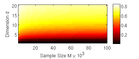
Figure 1: Heat map of predicted bias of non-averaged $f$-divergence estimator based on Theorem 2 as a function of dimension and sample size. Note the phase transition as dimension $d$ increases for fixed sample size $M$: bias remains small only for relatively small values of $d.$ The proposed weighted ensemble averaged estimator removes this phase transition when the densities are sufficiently smooth.

Theorem 3.

The variance of the plug-in estimator $\hat{\mathbf{G}}_{k_{1},k_{2}}$ is

$$\mathbb{V}\left[\hat{\mathbf{G}}_{k_{1},k_{2}}\right]=c_{9}\left(\frac{1}{N}\right)+c_{8,1}\left(\frac{1}{M_{1}}\right)+c_{8,2}\left(\frac{1}{M_{2}}\right)+o\left(\frac{1}{M_{1}}+\frac{1}{M_{2}}+\frac{1}{N}+\frac{1}{k_{1}^{2}}+\frac{1}{k_{2}^{2}}\right).$$

Note that the constants in front of the terms that depend on $k_{i}$ and $M_{i}$ are not identical for different $i$. However, these constants depend on the densities $f_{1}$ and $f_{2}$ which are often unknown and thus impossible to compute in practice. The rates given here are very similar to the rates derived for the entropy plug-in estimator in [13]. The differences are in the constants in front of the rates, the dependence on the number of samples from two distributions instead of one, and the $o\left(\frac{1}{k_{i}^{2}}\right)$ terms in the expression for the variance. The key to reducing mean squared error (MSE) is that by applying Theorem 1, the dependence of the MSE on $d$ will be greatly reduced.

III-B Weighted ensemble divergence estimator

Let $L>I=d-1$ and choose $\bar{l}=\left\{l_{1},\dots,l_{L}\right\}$ to be positive real numbers. Assume that $M_{1}=O\left(M_{2}\right).$ Let $k(l)=l\sqrt{M_{2}}$, $\hat{\mathbf{G}}_{k(l)}:=\hat{\mathbf{G}}_{k(l),k(l)},$ and $\hat{\mathbf{G}}_{w}:=\sum_{l\in\bar{l}}w(l)\hat{\mathbf{G}}_{k(l)}.$ From Theorems 2 and 3, the biases of the ensemble estimators $\left\{\hat{\mathbf{G}}_{k(l)}\right\}_{l\in\bar{l}}$ satisfy the condition $\mathcal{C}.1$ when $\psi_{i}(l)=l^{i/d}$ and $J=\{1,\dots,d-1\}$ since

$$\mathbb{B}\left(\hat{\mathbf{G}}_{k(l)}\right)=\sum_{j=1}^{d-1}O\left(l^{j/d}M_{2}^{-\frac{j}{2d}}\right)+O\left(\frac{1}{\sqrt{M_{2}}}\right).$$

The general form of the variance of $\hat{\mathbf{G}}_{k(l)}$ also follows $\mathcal{C}.2$ since $N,\,M_{2}=\Theta(T)$ (see $\mathcal{A}.0$). Thus we can find the optimal weight $w_{0}$ by using Theorem 1 to obtain a plug-in $f$-divergence estimator with convergence rate of $O\left(\frac{1}{T}\right).$

III-C Proofs of Theorems 2 and 3

Like for the case of entropy estimation studied in [13], the principal tools for the proofs of Theorems 2 and 3 are concentration inequalities and moment bounds applied to a higher order Taylor expansion of the functional (2). However, as the functional (2) depends on the ratio of densities, the analysis is more complicated than that of [13] since we have to bound the covariances between products of $\hat{\mathbf{e}}_{1,k_{1}}(\mathbf{Z})$ and $\hat{\mathbf{e}}_{2,k_{2}}(\mathbf{Z})$ where $\mathbf{Z}$ is drawn from $f_{2}$, $\hat{\mathbf{e}}_{i,k_{i}}(\mathbf{Z})=\hat{\mathbf{f}}_{i,k_{i}}(\mathbf{Z})-\mathbb{E}_{\mathbf{Z}}\hat{\mathbf{f}}_{i,k_{i}}(\mathbf{Z})$, and $\hat{\mathbf{F}}_{k_{1},k_{2}}(\mathbf{Z})=\hat{\mathbf{L}}_{k_{1},k_{2}}(\mathbf{Z})-\mathbb{E}_{\mathbf{Z}}\left(\hat{\mathbf{L}}_{k_{1},k_{2}}\right)$. Using Lemmas 5, 8, and 9 in [13], modified for application to $f_{1}$ and $f_{2}$, and two new Lemmas (Lemma 4 and Lemma 7 in the appendices) will establish Theorem 2 and Theorem 3. The modified versions of Lemmas 5 and 8 from [13] are given in Lemma 4 and Lemma 7, respectively while the modified version of Lemma 9 from [13] is given as Lemma 5. The details are given in Appendix A and Appendix B.

IV Experiments

To demonstrate the accuracy of the theoretical predictions of the performance of the ensemble method, we estimated the Rényi $\alpha$-divergence between two truncated normal densities with varying dimension and sample size restricted to the unit cube. The densities have means $\bar{\mu}_{1}=0.7*\bar{1}_{d}$, $\bar{\mu}_{2}=0.3*\bar{1}_{d}$ and covariance matrices $\sigma_{i}I_{d}$ where $\sigma_{1}=0.1,$ $\sigma_{2}=0.3,$ $\bar{1}_{d}$ is a $d$-dimensional vector of ones, and $I_{d}$ is a $d$-dimensional identity matrix. We used $\alpha=0.8$ and computed the estimates for the truncated kernel density plug-in estimate, the $k$-nn plug-in estimate, and the optimally weighted $k$-nn estimate. Since we have a finite number of samples, we obtain $w_{0}$ by solving the second convex optimization problem in [13] which introduces a slack variable on the bias constraint to better control the variance.

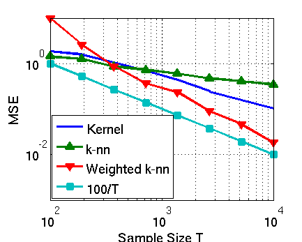
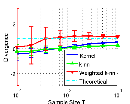
Figure 2: (Left) Log-log plot of MSE of the truncated uniform kernel and $k$-nn plug-in estimators (“Kernel”, “$k$-nn”), our proposed weighted ensemble estimator, and the theoretical bound from Theorem 1 scaled by a constant $(100/T)$. (Right) Average estimated divergence for each estimator with error bars indicating the standard deviation. Estimates for both plots are calculated from 100 trials for various sample sizes with fixed $d=5$. The proposed estimator outperforms the others for $T>400$ and is less biased.

The left plot in Fig. 2 shows the MSE of all three estimators for various sample sizes and fixed $d=5$. This experiment shows that the optimally weighted $k$-nn estimate consistently outperforms the others for sample sizes greater than $400$. The slope of the MSE of the optimally weighted $k$-nn estimate also matches the slope of the theoretical bound well.

The right plot in Fig. 2 shows the corresponding average estimated divergence and standard deviation for the three estimates. From the plot, the bias is consistently lowest for the ensemble estimate while the variance is highest suggesting that bias is decreased at the expense of increased variance.

We repeated the experiment with a fixed sample size of $T=3000$ and varying dimension. Based on the MSE, the ensemble estimate does better than the other methods for $d\geq 4$ and is comparable to the other methods for $d<4$ (see Fig. 3). Note that MSE appears to increase slightly for all estimators as $d$ increases. This is likely due to the dependence of the constants in the bias and variance terms on the densities and because we are using a fixed number of estimators $L$ [13].

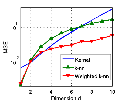
Figure 3: Plot of MSE of 100 trials of the estimators for various dimensions at a fixed sample size $T=3000$. The proposed estimator outperforms the others for $d\geq 4$ and performs similarly for $d\leq 3.$

To test the limits of our theoretical results, we also ran the experiment for non-truncated Gaussian random variables. Figure 4 shows the MSE as a function of sample size and dimension, respectively. For fixed $d=5,$ the weighted ensemble estimate has the lowest MSE for almost all sample sizes in the range considered. For fixed $T=3000,$ the MSE of the kernel plug-in method stays low for small dimension but then rapidly increases as $d$ increases. For the weighted $k$-nn method, the MSE increases at a slower rate as $d$ increases and is lowest for $d\leq 2$ and $d\geq 5.$

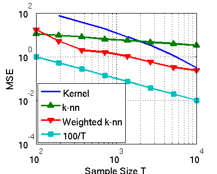
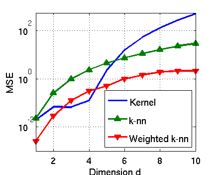
Figure 4: (Left) Log-log plot of MSE of the estimators for various sample sizes with fixed $d=5$ for the non-truncated case and the theoretical bound scaled by a constant $(100/T)$. (Right) Plot of MSE of the estimators for various dimensions at a fixed sample size $T=3000$ for the non-truncated case. 100 trials are used in both cases. The performance of the proposed estimator is similar to that of the truncated case.

V Conclusion

In this paper we derived convergence rates for a plug-in estimator of $f$-divergence using $d$-dimensional truncated $k$-nn density estimators. We then applied the theory of optimally weighted ensemble estimation to obtain an estimator with a convergence rate of $O\left(\frac{1}{T}\right)$. The advantages of this estimator is it is simple to implement, converges rapidly, and performs well for higher dimensions. This weighted ensemble divergence estimator also performs well for densities with unbounded support.

Appendix A Proof of Theorem 2

Note that $\mathbb{B}\left(\hat{\mathbf{G}}_{k_{1},k_{2}}\right)=\mathbb{E}\left[g\left(\hat{\mathbf{L}}_{k_{1},k_{2}}(\mathbf{Z})\right)-g\left(\mathbb{E}_{\mathbf{Z}}\hat{\mathbf{L}}_{k_{1},k_{2}}(\mathbf{Z})\right)\right]+\mathbb{E}\left[g\left(\mathbb{E}_{\mathbf{Z}}\hat{\mathbf{L}}_{k_{1},k_{2}}(\mathbf{Z})\right)-g\left(L(\mathbf{Z})\right)\right].$ We find bounds for these terms by using Taylor series expansions. The Taylor series expansion of $g\left(\hat{\mathbf{L}}_{k_{1},k_{2}}(\mathbf{Z})\right)$ around $\mathbb{E}_{\mathbf{Z}}\hat{\mathbf{L}}_{k_{1},k_{2}}(\mathbf{Z})$ gives

$$g\left(\hat{\mathbf{L}}_{k_{1},k_{2}}(\mathbf{Z})\right)=\sum_{i=0}^{2}\frac{g^{(i)}\left(\mathbb{E}_{\mathbf{Z}}\hat{\mathbf{L}}_{k_{1},k_{2}}(\mathbf{Z})\right)}{i!}\hat{\mathbf{F}}_{k_{1},k_{2}}^{i}(\mathbf{Z})+\frac{1}{6}g^{(3)}\left(\mathbf{\xi_{Z}}\right)\hat{\mathbf{F}}_{k_{1},k_{2}}^{3}(\mathbf{Z})$$ (3)

where $\mathbf{\xi_{Z}}\in\left(\mathbb{E}_{\mathbf{Z}}\hat{\mathbf{L}}_{k_{1},k_{2}}(\mathbf{Z}),\hat{\mathbf{L}}_{k_{1},k_{2}}(\mathbf{Z})\right)$ comes from the mean value theorem. The following lemma enables us to find bounds on the $\hat{\mathbf{F}}_{k_{1},k_{2}}^{i}$ terms:

Lemma 4.

Let $\gamma(z)$ be an arbitrary function with $\sup_{z}|\gamma(z)|<\infty.$ Let $\mathbf{Z}$ be a realization of the density $f_{2}$ independent of $\hat{\mathbf{f}}_{i,k_{i}}$ for $i=1,2$. Then,

$$\mathbb{E}\left[\gamma(\mathbf{Z})\hat{\mathbf{e}}_{i,k_{i}}^{q}(\mathbf{Z})\right] = \begin{cases}1_{\{q=2\}}\left(c_{2,i}(\gamma(z))\left(\frac{1}{k_{i}}\right)+o\left(\frac{1}{k_{i}}\right)\right)+1_{\{q\geq 3\}}O\left(\frac{1}{k_{i}^{\frac{q}{2}}}\right),&q\geq 2\\ 0,&q=1,\end{cases}$$ (4)

$$\mathbb{E}\left[\gamma(\mathbf{Z})\hat{\mathbf{e}}_{1,k_{1}}^{q}(\mathbf{Z})\hat{\mathbf{e}}_{2,k_{2}}^{r}(\mathbf{Z})\right] = \begin{cases}O\left(\frac{1}{k_{1}^{\frac{q}{2}}k_{2}^{\frac{r}{2}}}\right),&q,\,r\geq 2\\ 0,&q=1\,\text{or }r=1\end{cases}$$ (5)

$$\mathbb{E}\left[\gamma(\mathbf{Z})\hat{\mathbf{F}}_{k_{1},k_{2}}^{q}(\mathbf{Z})\right] = 1_{\{q=1\}}c_{4,1}\left(\frac{1}{k_{2}}\right)+1_{\{q=2\}}\left(c_{4,2}\left(\frac{1}{k_{2}}\right)+c_{4,3}\left(\frac{1}{k_{1}}\right)\right)+1_{\{q\geq 3\}}O\left(\frac{1}{k_{1}^{\frac{q}{2}}}+\frac{1}{k_{2}^{\frac{q}{2}}}\right)$$ (6)

$$= 1_{\{q=1\}}c_{4,1}\left(\frac{1}{k_{2}}\right)+1_{\{q=2\}}\left(c_{4,2}\left(\frac{1}{k_{2}}\right)+c_{4,3}\left(\frac{1}{k_{1}}\right)\right)+1_{\{q\geq 2\}}o\left(\frac{1}{k_{1}}\right)+o\left(\frac{1}{k_{2}}\right)$$

where $c_{2,i}$ and $c_{4,j}$ are functionals of $\gamma$, $f_{1},$ and $f_{2}.$

Proof.

For $i=2$, Eq. 4 is given and proved as Lemma 5 in [13] where the density estimator is a truncated uniform kernel density estimator with bandwidth $\left(k/M\right)^{1/d}$. The proof uses concentration inequalities to bound $\mathbb{E}_{\mathbf{Z}}\hat{\mathbf{e}}_{2,k_{2}}^{q}(\mathbf{Z})$ in terms of $k_{2}.$ It can then be shown that the $k$-nn density estimator converges to a truncated uniform kernel density estimator [21]. Thus the result holds for the $k$-nn density estimator as well. For $i=1,$ the proof follows the same procedure but results in a different constant.

For Eq. 5, note that for $q,\,r\geq 2,$

$$\mathbb{E}\left[\gamma(\mathbf{Z})\hat{\mathbf{e}}_{1,k_{1}}^{q}(\mathbf{Z})\hat{\mathbf{e}}_{2,k_{2}}^{r}(\mathbf{Z})\right] = \mathbb{E}\left[\gamma(\mathbf{Z})\mathbb{E}_{\mathbf{Z}}\left[\hat{\mathbf{e}}_{1,k_{1}}^{q}(\mathbf{Z})\hat{\mathbf{e}}_{2,k_{2}}^{r}(\mathbf{Z})\right]\right]$$

$$= \mathbb{E}\left[\gamma(\mathbf{Z})\mathbb{E}_{\mathbf{Z}}\left[\hat{\mathbf{e}}_{1,k_{1}}^{q}(\mathbf{Z})\right]\mathbb{E}_{\mathbf{Z}}\left[\hat{\mathbf{e}}_{2,k_{2}}^{r}(\mathbf{Z})\right]\right]$$

$$= \mathbb{E}\left[\gamma(\mathbf{Z})\left(O\left(\frac{1}{k_{1}^{\frac{q}{2}}k_{2}^{\frac{r}{2}}}\right)\right)\right]$$

$$= O\left(\frac{1}{k_{1}^{\frac{q}{2}}k_{2}^{\frac{r}{2}}}\right),$$

where we use conditional independence for the second equality and Eq. 4 for the third equality. If either $q=0$ or $r=0$ (but not both), then Eq. 5 reduces to Eq. 4.

For Eq. 6, we expand $\hat{\mathbf{L}}_{k_{1},k_{2}}(\mathbf{Z})$ around $\mathbb{E}_{\mathbf{Z}}\hat{\mathbf{f}}_{1,k_{1}}(\mathbf{Z})$ and $\mathbb{E}_{\mathbf{Z}}\hat{\mathbf{f}}_{2,k_{2}}(\mathbf{Z})$:

$$\frac{\hat{\mathbf{f}}_{1,k_{1}}(\mathbf{Z})}{\hat{\mathbf{f}}_{2,k_{2}}(\mathbf{Z})} = \frac{\mathbb{E}_{\mathbf{Z}}\hat{\mathbf{f}}_{1,k_{1}}(\mathbf{Z})}{\mathbb{E}_{\mathbf{Z}}\hat{\mathbf{f}}_{2,k_{2}}(\mathbf{Z})}+\frac{\hat{\mathbf{e}}_{1,k_{1}}(\mathbf{Z})}{\mathbb{E}_{\mathbf{Z}}\hat{\mathbf{f}}_{2,k_{2}}(\mathbf{Z})}-\mathbb{E}_{\mathbf{Z}}\hat{\mathbf{f}}_{1,k_{1}}(\mathbf{Z})\frac{\hat{\mathbf{e}}_{2,k_{2}}(\mathbf{Z})}{\left(\mathbb{E}_{\mathbf{Z}}\hat{\mathbf{f}}_{2,k_{2}}(\mathbf{Z})\right)^{2}}$$

$$-\frac{\hat{\mathbf{e}}_{1,k_{1}}(\mathbf{Z})\hat{\mathbf{e}}_{2,k_{2}}(\mathbf{Z})}{\left(\mathbb{E}_{\mathbf{Z}}\hat{\mathbf{f}}_{2,k_{2}}(\mathbf{Z})\right)^{2}}+\mathbb{E}_{\mathbf{Z}}\hat{\mathbf{f}}_{1,k_{1}}(\mathbf{Z})\frac{\hat{\mathbf{e}}_{2,k_{2}}^{2}(\mathbf{Z})}{2\left(\mathbb{E}_{\mathbf{Z}}\hat{\mathbf{f}}_{2,k_{2}}(\mathbf{Z})\right)^{3}}$$

$$+\frac{\hat{\mathbf{e}}_{1,k_{1}}(\mathbf{Z})\hat{\mathbf{e}}_{2,k_{2}}^{2}(\mathbf{Z})}{2\left(\mathbb{E}_{\mathbf{Z}}\hat{\mathbf{f}}_{2,k_{2}}(\mathbf{Z})\right)^{3}}+o\left(\hat{\mathbf{e}}_{2,k_{2}}^{2}(\mathbf{Z})+\hat{\mathbf{e}}_{1,k_{1}}(\mathbf{Z})\hat{\mathbf{e}}_{2,k_{2}}^{2}(\mathbf{Z})\right)$$

$$= \frac{\mathbb{E}_{\mathbf{Z}}\hat{\mathbf{f}}_{1,k_{1}}(\mathbf{Z})}{\mathbb{E}_{\mathbf{Z}}\hat{\mathbf{f}}_{2,k_{2}}(\mathbf{Z})}+h(\hat{\mathbf{e}}_{1,k_{1}}(\mathbf{Z}),\hat{\mathbf{e}}_{2,k_{2}}(\mathbf{Z})).$$

Let $\mathbf{h}(\mathbf{Z})=h(\hat{\mathbf{e}}_{1,k_{1}}(\mathbf{Z}),\hat{\mathbf{e}}_{2,k_{2}}(\mathbf{Z})).$ Thus $\hat{\mathbf{F}}_{k_{1},k_{2}}(\mathbf{Z})=\frac{\mathbb{E}_{\mathbf{Z}}\hat{\mathbf{f}}_{1,k_{1}}(\mathbf{Z})}{\mathbb{E}_{\mathbf{Z}}\hat{\mathbf{f}}_{2,k_{2}}(\mathbf{Z})}-\mathbb{E}_{\mathbf{Z}}\hat{\mathbf{L}}_{k_{1},k_{2}}(\mathbf{Z})+\mathbf{h}(\mathbf{Z}).$ By the binomial theorem,

$$\hat{\mathbf{F}}_{k_{1},k_{2}}^{q}(\mathbf{Z})=\sum_{j=0}^{q}a_{q,j}\left(\frac{\mathbb{E}_{\mathbf{Z}}\hat{\mathbf{f}}_{1,k_{1}}(\mathbf{Z})}{\mathbb{E}_{\mathbf{Z}}\hat{\mathbf{f}}_{2,k_{2}}(\mathbf{Z})}-\mathbb{E}_{\mathbf{Z}}\hat{\mathbf{L}}_{k_{1},k_{2}}(\mathbf{Z})\right)^{q-j}\mathbf{h}^{j}(\mathbf{Z}),$$ (8)

where $a_{q,j}$ is the binomial coefficient. From [13], $\mathbb{E}_{\mathbf{Z}}\hat{\mathbf{f}}_{i,k_{i}}(\mathbf{Z})=f_{i}(\mathbf{Z})+\sum_{j=1}^{d}c_{i,j,k_{i}}(\mathbf{Z})\left(\frac{k_{i}}{M_{i}}\right)^{j/d}+o\left(\frac{k_{i}}{M_{i}}\right)=f_{i}(\mathbf{Z})+c_{1,i}(\mathbf{Z},k_{i},M_{i})=f_{i}(\mathbf{Z})+o(1).$ This quantity is bounded above and below based on our assumptions. Using a Taylor series expansion of $\frac{1}{x}$ about $\mathbb{E}_{\mathbf{Z}}\hat{\mathbf{f}}_{2,k_{2}}(\mathbf{Z})$,

$$\mathbb{E}_{\mathbf{Z}}\frac{1}{\hat{\mathbf{f}}_{2,k_{2}}(\mathbf{Z})} = \mathbb{E}_{\mathbf{Z}}\left[\frac{1}{\mathbb{E}_{\mathbf{Z}}\hat{\mathbf{f}}_{2,k_{2}}(\mathbf{Z})}-\frac{\hat{\mathbf{e}}_{2,k_{2}}}{\left(\mathbb{E}_{\mathbf{Z}}\hat{\mathbf{f}}_{2,k_{2}}(\mathbf{Z})\right)^{2}}+\frac{\hat{\mathbf{e}}_{2,k_{2}}^{2}}{2\xi_{2,\mathbf{Z}}}\right]$$ (9)

$$= \frac{1}{\mathbb{E}_{\mathbf{Z}}\hat{\mathbf{f}}_{2,k_{2}}(\mathbf{Z})}+\frac{\left(\mathbb{V}_{\mathbf{Z}}\left[\hat{\mathbf{f}}_{2,k_{2}}(\mathbf{Z})\right]\right)}{2\xi_{2,\mathbf{Z}}}$$

$$= \frac{1}{\mathbb{E}_{\mathbf{Z}}\hat{\mathbf{f}}_{2,k_{2}}(\mathbf{Z})}+c_{3,2}(\mathbf{Z})\left(\frac{1}{k_{2}}\right),$$

where $\xi_{2,\mathbf{Z}}\in\left(\mathbb{E}_{\mathbf{Z}}\hat{\mathbf{f}}_{2,k_{2}}(\mathbf{Z}),\hat{\mathbf{f}}_{2,k_{2}}(\mathbf{Z})\right)$ from the mean value thoerem and we use the fact that the variance of the kernel density estimate converges to zero with rate $\frac{1}{M_{2}\sigma_{2}}$ where $\sigma_{2}=O\left(\frac{k_{2}}{M_{2}}\right)$. Thus

$$\left(\frac{\mathbb{E}_{\mathbf{Z}}\hat{\mathbf{f}}_{1,k_{1}}(\mathbf{Z})}{\mathbb{E}_{\mathbf{Z}}\hat{\mathbf{f}}_{2,k_{2}}(\mathbf{Z})}-\mathbb{E}_{\mathbf{Z}}\hat{\mathbf{L}}_{k_{1},k_{2}}(\mathbf{Z})\right)^{q} = \left(\mathbb{E}_{\mathbf{Z}}\hat{\mathbf{f}}_{1,k_{1}}(\mathbf{Z})c_{3,2}(\mathbf{Z})\left(\frac{1}{k_{2}}\right)\right)^{q}$$ (10)

$$= \left(f_{1}(\mathbf{Z})c_{3,2}(\mathbf{Z})\left(\frac{1}{k_{2}}\right)+\sum_{j=1}^{d}c_{1,j,k_{1}}\left(\frac{k_{1}}{M_{1}}\right)^{\frac{j}{d}}\left(\frac{1}{k_{2}}\right)+o\left(\frac{k_{1}}{M_{1}k_{2}}\right)\right)^{q}$$

$$= 1_{\{q=1\}}c_{3}(\mathbf{Z})\left(\frac{1}{k_{2}}\right)+1_{\{q\geq 2\}}O\left(\frac{1}{k_{2}^{q}}\right)+o\left(\frac{1}{k_{2}^{q}}\right)=:b_{q,k_{2}}(\mathbf{Z}).$$

This is also bounded. Combining Eqs. 8 and 10:

$$\hat{\mathbf{F}}_{k_{1},k_{2}}^{q}(\mathbf{Z}) = b_{q,k_{2}}(\mathbf{Z})+b_{q-1,k_{2}}^{1_{\{q\geq 2\}}}(\mathbf{Z})a_{q,1}\mathbf{h}(\mathbf{Z})+1_{\{q\geq 2\}}b_{q-2,k_{2}}^{1_{\{q\geq 3\}}}(\mathbf{Z})a_{q,2}\mathbf{h}^{2}(\mathbf{Z})+1_{\{q\geq 3\}}b_{q-3,k_{2}}^{1_{\{q\geq 4\}}}(\mathbf{Z})O\left(\mathbf{h}^{3}(\mathbf{Z})\right)$$ (11)

$$= b_{q,k_{2}}(\mathbf{Z})+b_{q-1,k_{2}}^{1_{\{q\geq 2\}}}(\mathbf{Z})a_{q,1}\times$$

$$\left(\frac{\hat{\mathbf{e}}_{1,k_{1}}(\mathbf{Z})}{\mathbb{E}_{\mathbf{Z}}\hat{\mathbf{f}}_{2,k_{2}}(\mathbf{Z})}-\frac{\mathbb{E}_{\mathbf{Z}}\hat{\mathbf{f}}_{1,k_{1}}(\mathbf{Z})}{\left(\mathbb{E}_{\mathbf{Z}}\hat{\mathbf{f}}_{2,k_{2}}(\mathbf{Z})\right)^{2}}\hat{\mathbf{e}}_{2,k_{2}}(\mathbf{Z})-\frac{\hat{\mathbf{e}}_{1,k_{1}}(\mathbf{Z})\hat{\mathbf{e}}_{2,k_{2}}(\mathbf{Z})}{\left(\mathbb{E}_{\mathbf{Z}}\hat{\mathbf{f}}_{2,k_{2}}(\mathbf{Z})\right)^{2}}+\frac{\mathbb{E}_{\mathbf{Z}}\hat{\mathbf{f}}_{1,k_{1}}(\mathbf{Z})}{2\left(\mathbb{E}_{\mathbf{Z}}\hat{\mathbf{f}}_{2,k_{2}}(\mathbf{Z})\right)^{3}}\hat{\mathbf{e}}_{2,k_{2}}^{2}(\mathbf{Z})+o\left(\hat{\mathbf{e}}_{2,k_{2}}^{2}(\mathbf{Z})\right)\right)$$

$$+1_{\{q\geq 2\}}b_{q-2,k_{2}}^{1_{\{q\geq 3\}}}(\mathbf{Z})a_{q,2}\left(\frac{\hat{\mathbf{e}}_{1,k_{1}}^{2}(\mathbf{Z})}{\left(\mathbb{E}_{\mathbf{Z}}\hat{\mathbf{f}}_{2,k_{2}}(\mathbf{Z})\right)^{2}}+\frac{\left(\mathbb{E}_{\mathbf{Z}}\hat{\mathbf{f}}_{1,k_{1}}(\mathbf{Z})\right)^{2}}{\left(\mathbb{E}_{\mathbf{Z}}\hat{\mathbf{f}}_{2,k_{2}}(\mathbf{Z})\right)^{4}}\hat{\mathbf{e}}_{2,k_{2}}^{2}(\mathbf{Z})+O\left(\hat{\mathbf{e}}_{1,k_{1}}(\mathbf{Z})\hat{\mathbf{e}}_{2,k_{2}}(\mathbf{Z})+\hat{\mathbf{e}}_{2,k_{2}}^{3}(\mathbf{Z})\right)\right)$$

$$+1_{\{q\geq 3\}}b_{q-2,k_{2}}^{1_{\{q\geq 4\}}}(\mathbf{Z})\left(O\left(\hat{\mathbf{e}}_{1,k_{1}}^{3}(\mathbf{Z})+\hat{\mathbf{e}}_{2,k_{2}}^{3}(\mathbf{Z})+\hat{\mathbf{e}}_{1,k_{1}}^{2}(\mathbf{Z})\hat{\mathbf{e}}_{2,k_{2}}^{2}(\mathbf{Z})\right)\right)$$

$$= b_{q,k_{2}}(\mathbf{Z})+\sum_{i=1}^{3}\mathbf{u}_{i,q}(\mathbf{Z}).$$

Applying Eqs. 4 and 5 we have

$$\mathbb{E}\left[\gamma(\mathbf{Z})\hat{\mathbf{F}}_{k_{1},k_{2}}^{q}(\mathbf{Z})\right] = \left(1_{\{q=1\}}\left(\mathbb{E}\left[\gamma(\mathbf{Z})c_{3}(\mathbf{Z})\right]+c_{2,2}\left(\frac{\gamma(z)\mathbb{E}_{Z}\hat{\mathbf{f}}_{1,k_{1}}(z)}{2\left(\mathbb{E}_{Z}\hat{\mathbf{f}}_{2,k_{2}}(z)\right)^{3}}\right)\right)+1_{\{q=2\}}c_{2,2}\left(\frac{\gamma(z)\left(\mathbb{E}_{Z}\hat{\mathbf{f}}_{1,k_{1}}(z)\right)^{2}}{\left(\mathbb{E}_{Z}\hat{\mathbf{f}}_{2,k_{2}}(z)\right)^{4}}\right)\right)\left(\frac{1}{k_{2}}\right)$$

$$+1_{\{q=2\}}c_{2,1}\left(\frac{\gamma(z)}{\left(\mathbb{E}_{Z}\hat{\mathbf{f}}_{2,k_{2}}(z)\right)^{2}}\right)\left(\frac{1}{k_{1}}\right)+1_{\{q\geq 2\}}o\left(\frac{1}{k_{1}}\right)+o\left(\frac{1}{k_{2}}\right)$$

$$= 1_{\{q=1\}}c_{4,1}\left(\frac{1}{k_{2}}\right)+1_{\{q=2\}}\left(c_{4,2}\left(\frac{1}{k_{2}}\right)+c_{4,3}\left(\frac{1}{k_{1}}\right)\right)+1_{\{q\geq 2\}}o\left(\frac{1}{k_{1}}\right)+o\left(\frac{1}{k_{2}}\right).$$

Then since $\mathbb{E}_{Z}\hat{\mathbf{f}}_{i,k_{i}}(Z)=f_{i}(Z)+o(1)$, the constants depend on $f_{1},$ $f_{2}$, and $\gamma.$

To obtain the more general bound for $\mathbb{E}\left[\gamma(\mathbf{Z})\hat{\mathbf{F}}_{k_{1},k_{2}}^{q}(\mathbf{Z})\right]$, note that from Eqs. 4, 5, and A, the leading terms $\mathbb{E}_{\mathbf{Z}}\mathbf{h}^{q}(\mathbf{Z})$ with $q<4$ are

$$\mathbb{E}_{\mathbf{Z}}\mathbf{h}^{q}(\mathbf{Z})=\begin{cases}O\left(\frac{1}{k_{2}}\right),&q=1,\\ O\left(\frac{1}{k_{1}^{\frac{q}{2}}}+\frac{1}{k_{2}^{\frac{q}{2}}}+\frac{1}{k_{1}k_{2}}\right),&q=2,\,3.\end{cases}$$

Note that $O\left(\frac{1}{k_{1}k_{2}}\right)=O\left(\frac{1}{\left(\min\left(k_{1},k_{2}\right)\right)^{2}}\right)$. Thus for $q=2,\,3,$ we ignore this term to get $\mathbb{E}_{\mathbf{Z}}\mathbf{h}^{q}(\mathbf{Z})=O\left(\frac{1}{k_{1}^{q/2}}+\frac{1}{k_{2}^{q/2}}\right).$ For $q\geq 4$, the leading terms come from products of powers of $\hat{\mathbf{e}}_{1,k_{1}}$ and $\hat{\mathbf{e}}_{2,k_{2}}.$ This gives

$$\mathbb{E}_{\mathbf{Z}}\mathbf{h}^{q}(\mathbf{Z}) = O\left(\frac{1}{k_{1}^{\frac{q}{2}}}+\frac{1}{k_{2}^{\frac{q}{2}}}+\sum_{\begin{subarray}{c}i+j=q\\ i,j\geq 2\end{subarray}}\frac{1}{k_{1}^{\frac{i}{2}}k_{2}^{\frac{j}{2}}}\right)$$

$$= O\left(\frac{1}{k_{1}^{\frac{q}{2}}}+\frac{1}{k_{2}^{\frac{q}{2}}}+\sum_{\begin{subarray}{c}i+j=q\\ i,j\geq 2\end{subarray}}\frac{1}{\left(\min\left(k_{1},k_{2}\right)\right)^{\frac{i+j}{2}}}\right)$$

$$= O\left(\frac{1}{k_{1}^{\frac{q}{2}}}+\frac{1}{k_{2}^{\frac{q}{2}}}\right)$$

$$\implies\mathbb{E}\left[\gamma(\mathbf{Z})\hat{\mathbf{F}}_{k_{1},k_{2}}^{q}(\mathbf{Z})\right] = \sum_{j=0}^{q}O\left(\frac{1}{k_{2}^{q-j}}\right)\mathbb{E}\left[\mathbb{E}_{\mathbf{Z}}\mathbf{h}^{j}(\mathbf{Z})\right]$$

$$= 1_{\{q=1\}}O\left(\frac{1}{k_{2}}\right)+1_{\{q\geq 2\}}O\left(\frac{1}{k_{1}^{\frac{q}{2}}}+\frac{1}{k_{2}^{\frac{q}{2}}}\right).$$

∎

The following lemma is required to bound the $g^{(3)}\left(\mathbf{\xi_{Z}}\right)$ term.

Lemma 5.

Assume that U(x) is any arbitrary functional which satisfies

$$(i) \mathbb{E}\left[\sup_{L\in(p_{l},p_{u})}\left|U\left(L\frac{\mathbf{p}_{2}}{\mathbf{p}_{1}}\right)\right|\right]=G_{1}<\infty,$$

$$(ii) \sup_{L\in\left(\frac{q_{l,1}}{q_{u,2}},\frac{q_{u,1}}{q_{l,2}}\right)}\left|U\left(L\right)\right|\mathcal{C}\left(k_{1}\right)\mathcal{C}\left(k_{2}\right)=G_{2}<\infty,$$

$$(iii) \mathbb{E}\left[\sup_{L\in\left(\frac{q_{l,1}}{p_{u,2}},\frac{q_{u,1}}{p_{l,2}}\right)}\left|U\left(L\mathbf{p}_{2}\right)\right|\mathcal{C}\left(k_{1}\right)\right]=G_{3}<\infty,$$

$$(iv) \mathbb{E}\left[\sup_{L\in\left(\frac{p_{l,1}}{q_{u,2}},\frac{p_{u,1}}{q_{l,2}}\right)}\left|U\left(\frac{L}{\mathbf{p}_{1}}\right)\right|\mathcal{C}\left(k_{2}\right)\right]=G_{4}<\infty.$$

Let $\mathbf{Z}$ be $\mathbf{X}_{i}$ for some fixed $i\in\{1,\dots,N\}$ and $\xi_{\mathbf{Z}}$ be any random variable which almost surely lies in $(L(\mathbf{Z}),\hat{\mathbf{L}}_{k_{1},k_{2}}(\mathbf{Z})).$ Then $\mathbb{E}|U(\xi_{\mathbf{Z}})|<\infty.$

Proof.

This is a version of Lemma 9 in [13] modified to apply to functionals of the likelihood ratio. Because of assumption $\mathcal{A}.1$, it is sufficient to show that the conditional expectation $\mathbb{E}\left[|U(\xi_{Z})|\,|\,\mathbf{X}_{1},\dots,\mathbf{X}_{N}\right]<\infty.$

First, some properties of $k$-NN density estimators are required. Let $\mathbf{S}_{k_{i},i}(Z)=\left\{Y:d(Z,Y)\leq\mathbf{d}_{Z,i}^{(k_{i})}\right\}$ where $\mathbf{d}_{Z,i}^{(k_{i})}$ is the distance to the $k_{i}$th nearest neighbor of $Z$ from the corresponding set of samples. Then let $\mathbf{P}_{i}(Z)=\int_{\mathbf{S}_{k_{i},i}(Z)}f_{i}(x)dx$ which has a beta distribution with parameters $k_{i}$ and $M_{i}-k_{i}+1$ [22]. Let $A_{i}(Z)$ be the event that $\mathbf{P}_{i}(Z)<\left(\frac{\sqrt{6}}{k_{i}^{\delta/2}}+1\right)\frac{k_{i}-1}{M_{i}}.$ It has been shown that $Pr\left(A_{i}(Z)^{C}\right)=\Theta\left(\mathcal{C}\left(k_{i}\right)\right)$ and that under $A_{i}(Z)$ [21, 23],

$$\frac{p_{l,i}}{\mathbf{P}_{i}(Z)}<\hat{\mathbf{f}}_{i,k_{i}}(Z)<\frac{p_{u,i}}{\mathbf{P}_{i}(Z)}.$$

It has also been shown that under $A_{i}(Z)^{C}$ [21, 23],

$$q_{l,i}<\hat{\mathbf{f}}_{i,k_{i}}(Z)<q_{u,i}.$$

Let $A(Z)=A_{1}(Z)\cap A_{2}(Z)$ and note that $A_{1}(Z)$ and $A_{2}(Z)$ are independent events. Thus since $\hat{\mathbf{L}}_{k_{1},k_{2}}(Z)=\frac{\hat{\mathbf{f}}_{1,k_{1}}(Z)}{\hat{\mathbf{f}}_{2,k_{2}}(Z)},$ we have that under $A(Z),$

$$p_{l}\frac{\mathbf{P}_{2}(Z)}{\mathbf{P}_{1}(Z)}<\hat{\mathbf{L}}_{k_{1},k_{2}}(Z)<p_{u}\frac{\mathbf{P}_{2}(Z)}{\mathbf{P}_{1}(Z)}.$$

Now let $Q_{1}(Z)=A_{1}(Z)^{C}\cap A_{2}(Z)^{C},$ $Q_{2}(Z)=A_{1}(Z)^{C}\cap A_{2}(Z),$ and $Q_{3}(Z)=A_{1}(Z)\cap A_{2}(Z)^{C}.$ Then due to independence and the fact that the $Q_{i}(Z)$s are disjoint,

$$A(Z)^{C} = A_{1}(Z)^{C}\cup A_{2}(Z)^{C}=Q_{1}(Z)\cup Q_{2}(Z)\cup Q_{3}(Z),$$

$$\implies Pr\left(A(Z)^{C}\right) = Pr\left(Q_{1}(Z)\right)+Pr\left(Q_{2}(Z)\right)+Pr\left(Q_{3}(Z)\right)$$

$$\leq \mathcal{C}\left(k_{1}\right)\mathcal{C}\left(k_{2}\right)+\mathcal{C}\left(k_{1}\right)+\mathcal{C}\left(k_{2}\right).$$

Then under $Q_{1}(Z)$, $Q_{2}(Z),$ and $Q_{3}(Z)$, respectively,

$$\frac{q_{l,1}}{q_{u,2}}<\hat{\mathbf{L}}_{k_{1},k_{2}}(Z)<\frac{q_{u,1}}{q_{l,2}},$$

$$\frac{q_{l,1}\mathbf{P}_{2}(Z)}{p_{u,2}}<\hat{\mathbf{L}}_{k_{1},k_{2}}(Z)<\frac{q_{u,1}\mathbf{P}_{2}(Z)}{p_{l,2}},$$

$$\frac{p_{l,1}}{\mathbf{P}_{1}(Z)q_{u,2}}<\hat{\mathbf{L}}_{k_{1},k_{2}}(Z)<\frac{p_{u,1}}{\mathbf{P}_{1}(Z)q_{l,2}}.$$

Conditioning on $\mathbf{X}_{1},\dots,\mathbf{X}_{N}$ gives

$$\mathbb{E}\left[\left|U(\xi_{Z})\right|\right] = \mathbb{E}\left[1_{A(Z)}\left|U(\xi_{Z})\right|\right]+\mathbb{E}\left[1_{Q_{1}(Z)}\left|U(\xi_{Z})\right|\right]+\mathbb{E}\left[1_{Q_{2}(Z)}\left|U(\xi_{Z})\right|\right]+\mathbb{E}\left[1_{Q_{3}(Z)}\left|U(\xi_{Z})\right|\right]$$

$$\leq Pr(A(Z))\mathbb{E}\left[\sup_{L\in(p_{l},p_{u})}\left|U\left(L\frac{\mathbf{P}_{2}(Z)}{\mathbf{P}_{1}(Z)}\right)\right|\right]+Pr(Q_{1}(Z))\sup_{L\in\left(\frac{q_{l,1}}{q_{u,2}},\frac{q_{u,1}}{q_{l,2}}\right)}\left|U\left(L\right)\right|$$

$$+Pr(Q_{1}(Z))\mathbb{E}\left[\sup_{L\in\left(\frac{q_{l,1}}{p_{u,2}},\frac{q_{u,1}}{p_{l,2}}\right)}\left|U\left(L\mathbf{P}_{2}(Z)\right)\right|\right]+Pr(Q_{1}(Z))\mathbb{E}\left[\sup_{L\in\left(\frac{p_{l,1}}{q_{u,2}},\frac{p_{u,1}}{q_{l,2}}\right)}\left|U\left(\frac{L}{\mathbf{P}_{1}(Z)}\right)\right|\right]$$

$$\leq \mathbb{E}\left[\sup_{L\in(p_{l},p_{u})}\left|U\left(L\frac{\mathbf{P}_{2}(Z)}{\mathbf{P}_{1}(Z)}\right)\right|\right]+\sup_{L\in\left(\frac{q_{l,1}}{q_{u,2}},\frac{q_{u,1}}{q_{l,2}}\right)}\left|U\left(L\right)\right|\mathcal{C}\left(k_{1}\right)\mathcal{C}\left(k_{2}\right)$$

$$+\mathbb{E}\left[\sup_{L\in\left(\frac{q_{l,1}}{p_{u,2}},\frac{q_{u,1}}{p_{l,2}}\right)}\left|U\left(L\mathbf{P}_{2}(Z)\right)\right|\mathcal{C}\left(k_{1}\right)\right]+\mathbb{E}\left[\sup_{L\in\left(\frac{p_{l,1}}{q_{u,2}},\frac{p_{u,1}}{q_{l,2}}\right)}\left|U\left(\frac{L}{\mathbf{P}_{1}(Z)}\right)\right|\mathcal{C}\left(k_{2}\right)\right]$$

$$= G_{1}+G_{2}+G_{3}+G_{4}<\infty.$$

∎

Applying Lemma 5 and assumption $(\mathcal{A}.5)$ gives $\mathbb{E}\left[\left(g^{(3)}\left(\xi_{\mathbf{Z}}\right)/6\right)^{2}\right]=O(1).$ Then by Cauchy-Schwarz and applying Lemma 4,

$$\mathbb{E}\left[\frac{1}{6}g^{(3)}\left(\mathbf{\xi_{Z}}\right)\hat{\mathbf{F}}_{k_{1},k_{2}}^{3}(\mathbf{Z})\right]\leq\sqrt{\mathbb{E}\left[\left(\frac{g^{(3)}\left(\xi_{\mathbf{Z}}\right)}{6}\right)^{2}\right]\mathbb{E}\left[\hat{\mathbf{F}}_{k_{1},k_{2}}^{6}(\mathbf{Z})\right]}=o\left(\frac{1}{k_{1}}+\frac{1}{k_{2}}\right).$$

Using this result with Eq. 3 and applying Lemma 4 again gives

$$\mathbb{E}\left[g\left(\hat{\mathbf{L}}_{k_{1},k_{2}}(\mathbf{Z})\right)-g\left(\mathbb{E}_{\mathbf{Z}}\hat{\mathbf{L}}_{k_{1},k_{2}}(\mathbf{Z})\right)\right]=\left(c_{4,1}+c_{4,2}\right)\left(\frac{1}{k_{2}}\right)+c_{4,3}\left(\frac{1}{k_{1}}\right)+o\left(\frac{1}{k_{1}}+\frac{1}{k_{2}}\right).$$ (12)

Now by Taylor series expansion

$$g\left(\mathbb{E}_{\mathbf{Z}}\hat{\mathbf{L}}_{k_{1},k_{2}}(\mathbf{Z})\right)=g\left(L(\mathbf{Z})\right)+\sum_{i=1}^{d}g^{(i)}\left(L(\mathbf{Z})\right)\left(\mathbb{E}_{\mathbf{Z}}\hat{\mathbf{L}}_{k_{1},k_{2}}(\mathbf{Z})-L(\mathbf{Z})\right)^{i}+o\left(\left(\mathbb{E}_{\mathbf{Z}}\hat{\mathbf{L}}_{k_{1},k_{2}}(\mathbf{Z})-L(\mathbf{Z})\right)^{d}\right).$$

From Eq. 9,

$$\mathbb{E}_{\mathbf{Z}}\hat{\mathbf{L}}_{k_{1},k_{2}}(\mathbf{Z})-L(\mathbf{Z}) = \mathbb{E}_{\mathbf{Z}}\hat{\mathbf{f}}_{1,k_{1}}(\mathbf{Z})\left(\frac{1}{f_{2}(\mathbf{Z})+c_{1,2}(\mathbf{Z},k_{2},M_{2})}+c_{3,2}(\mathbf{Z})\left(\frac{1}{k_{2}}\right)\right)-L(\mathbf{Z})$$

$$= \frac{f_{2}(\mathbf{Z})c_{1,1}(\mathbf{Z},k_{1},M_{1})-f_{1}(\mathbf{Z})c_{1,2}(\mathbf{Z},k_{1},M_{2})}{f_{2}(\mathbf{Z})\left(f_{2}(\mathbf{Z})+c_{1,2}(\mathbf{Z},k_{2},M_{2})\right)}+\mathbb{E}_{\mathbf{Z}}\hat{\mathbf{f}}_{1,k_{1}}(\mathbf{Z})c_{3,2}(\mathbf{Z})\left(\frac{1}{k_{2}}\right)$$

$$= \frac{c_{1,1}(\mathbf{Z},k_{1},M_{1})}{f_{2}(\mathbf{Z})+o(1)}-\frac{f_{1}(\mathbf{Z})c_{1,2}(\mathbf{Z},k_{2},M_{2})}{f_{2}(\mathbf{Z})\left(f_{2}(\mathbf{Z})+o(1)\right)}+\mathbb{E}_{\mathbf{Z}}\hat{\mathbf{f}}_{1,k_{1}}(\mathbf{Z})c_{3,2}(\mathbf{Z})\left(\frac{1}{k_{2}}\right)$$

$$= \sum_{j=1}^{d}\left(c_{5,j,1}(\mathbf{Z})\left(\frac{k_{1}}{M_{1}}\right)^{\frac{j}{d}}+c_{5,j,2}(\mathbf{Z})\left(\frac{k_{2}}{M_{2}}\right)^{\frac{j}{d}}\right)+f_{1}(\mathbf{Z})c_{3,2}(\mathbf{Z})\left(\frac{1}{k_{2}}\right)+o\left(\frac{k_{1}}{M_{1}}+\frac{k_{2}}{M_{2}}+\frac{1}{k_{2}}\right).$$

This gives

$$\mathbb{E}\left[g\left(\mathbb{E}_{\mathbf{Z}}\hat{\mathbf{L}}_{k}(\mathbf{Z})\right)-g\left(L(\mathbf{Z})\right)\right]=\sum_{j=1}^{d}\left(c_{6,j,1}\left(\frac{k_{1}}{M_{1}}\right)^{\frac{j}{d}}+c_{6,j,2}\left(\frac{k_{2}}{M_{2}}\right)^{\frac{j}{d}}\right)+c_{6,3}\left(\frac{1}{k_{2}}\right)+o\left(\frac{k_{1}}{M_{1}}+\frac{k_{2}}{M_{2}}+\frac{1}{k_{2}}\right),$$ (13)

where $c_{6,3}=\mathbb{E}\left[g^{\prime}\left(L(\mathbf{Z})\right)f_{1}(\mathbf{Z})c_{3,2}(\mathbf{Z})\right]$ and $c_{6,j,i}$ is a functional of $g$, the derivatives of $g$, and the densities $f_{1}$ and $f_{2}$.

Combining Eqs. 12 and 13 completes the proof.

Appendix B Proof of Theorem 3

Again, we start by forming a Taylor series expansion of $g\left(\hat{\mathbf{L}}_{k_{1},k_{2}}(\mathbf{Z})\right)$ around $\mathbb{E}_{\mathbf{Z}}\hat{\mathbf{L}}_{k_{1},k_{2}}(\mathbf{Z})$.

$$g\left(\hat{\mathbf{L}}_{k_{1},k_{2}}(\mathbf{Z})\right)=\sum_{i=0}^{\lambda-1}\frac{g^{(i)}\left(\mathbb{E}_{\mathbf{Z}}\hat{\mathbf{L}}_{k_{1},k_{2}}(\mathbf{Z})\right)}{i!}\hat{\mathbf{F}}_{k_{1},k_{2}}^{i}(\mathbf{Z})+\frac{g^{(\lambda)}\left(\mathbf{\xi_{Z}}\right)}{\lambda!}\hat{\mathbf{F}}_{k_{1},k_{2}}^{\lambda}(\mathbf{Z}),$$

where $\mathbf{\xi_{Z}}\in\left(\mathbb{E}_{\mathbf{Z}}\hat{\mathbf{L}}_{k_{1},k_{2}}(\mathbf{Z}),\hat{\mathbf{L}}_{k_{1},k_{2}}(\mathbf{Z})\right)$. Let $\Psi(\mathbf{Z})=g^{(\lambda)}\left(\mathbf{\xi_{Z}}\right)/\lambda!$ and define the operator $\mathcal{M}(\mathbf{Z})=\mathbf{Z}-\mathbb{E}\mathbf{Z}.$ Let

$$\mathbf{p}_{i} = \mathcal{M}\left(g\left(\mathbb{E}_{\mathbf{X}_{i}}\hat{\mathbf{L}}_{k_{1},k_{2}}\left(\mathbf{X}_{i}\right)\right)\right),$$

$$\mathbf{q}_{i} = \mathcal{M}\left(g^{\prime}\left(\mathbb{E}_{\mathbf{X}_{i}}\hat{\mathbf{L}}_{k_{1},k_{2}}\left(\mathbf{X}_{i}\right)\right)\hat{\mathbf{F}}_{k_{1},k_{2}}\left(\mathbf{X}_{i}\right)\right),$$

$$\mathbf{r}_{i} = \mathcal{M}\left(\sum_{j=2}^{\lambda-1}\frac{g^{(j)}\left(\mathbb{E}_{\mathbf{X}_{i}}\hat{\mathbf{L}}_{k_{1},k_{2}}\left(\mathbf{X}_{i}\right)\right)}{j!}\hat{\mathbf{F}}_{k_{1},k_{2}}^{j}\left(\mathbf{X}_{i}\right)\right)$$

$$\mathbf{s}_{i} = \mathcal{M}\left(\Psi\left(\mathbf{X}_{i}\right)\hat{\mathbf{F}}_{k_{1},k_{2}}^{\lambda}\left(\mathbf{X}_{i}\right)\right).$$

Then the variance of $\hat{\mathbf{G}}_{k_{1},k_{2}}$ is

$$\mathbb{V}\left(\hat{\mathbf{G}}_{k_{1},k_{2}}\right) = \mathbb{E}\left[\left(\hat{\mathbf{G}}_{k_{1},k_{2}}-\mathbb{E}\hat{\mathbf{G}}_{k_{1},k_{2}}\right)^{2}\right]$$

$$= \frac{1}{N}\mathbb{E}\left[\left(\mathbf{p}_{1}+\mathbf{q}_{1}+\mathbf{r}_{1}+\mathbf{s}_{1}\right)^{2}\right]+\frac{N-1}{N}\mathbb{E}\left[\left(\mathbf{p}_{1}+\mathbf{q}_{1}+\mathbf{r}_{1}+\mathbf{s}_{1}\right)\left(\mathbf{p}_{2}+\mathbf{q}_{2}+\mathbf{r}_{2}+\mathbf{s}_{2}\right)\right].$$

We will bound this using Lemma 4 and the following lemmas.

Lemma 6.

Let $\Psi_{i}=\left\{\{X,Y\}:\left\|X-Y\right\|_{1}\geq 2\left(\frac{k_{i}}{M_{i}}\right)^{\frac{1}{d}}\right\}.$ For a fixed pair of points $\{X,Y\}\in\Psi_{i}$, and positive integers $q,$ $r,$

$$Cov\left[\hat{\mathbf{e}}_{i,k_{i}}^{q}(X),\hat{\mathbf{e}}_{i,k_{i}}^{r}(Y)\right]=1_{\{q=r=1\}}\left(\frac{-f_{i}(X)f_{i}(Y)}{M_{i}}\right)+o\left(\frac{1}{M_{i}}\right).$$

For a fixed pair of points $\{X,Y\}\in\Psi_{i}^{C},$

$$Cov\left[\hat{\mathbf{e}}_{i,k_{i}}^{q}(X),\hat{\mathbf{e}}_{i,k_{i}}^{r}(Y)\right]=1_{\{q=r=1\}}O\left(\frac{1}{k_{i}}\right)+o\left(\frac{1}{k_{i}}\right).$$

This lemma is given and proved as Lemmas 6 and 7 in [13] for the truncated uniform kernel density estimator using concentration inequalities and Eq. 4. Thus the result holds for the $k$-nn density estimator as well.

Lemma 7.

Let $\gamma_{1}(x),$ $\gamma_{2}(x)$ be arbitrary functions with $1$ partial derivative wrt $x$ and $\sup_{x}|\gamma_{i}(x)|<\infty,\,i=1,\,2.$ Let $\mathbf{X},$ $\mathbf{Y}$ be realizations of the density $f_{2}$ independent of the realizations used for $\hat{\mathbf{f}}_{1,k_{1}}$ and $\hat{\mathbf{f}}_{2,k_{2}}$. Let $E_{0}=\{s,q,t,r\geq 1\}$, $E_{1,1}=\{s=0,q\geq 2,t\geq 1,r\geq 1\}\cup\{s\geq 1,q\geq 1,t=0,r\geq 2\}$, and $E_{1,2}=\{s\geq 2,q=0,t\geq 1,r\geq 1\}\cup\{s\geq 1,q\geq 1,t\geq 2,r=0\}$. Then

$$Cov\left[\gamma_{1}(\mathbf{X})\hat{\mathbf{e}}_{i,k_{i}}^{q}(\mathbf{X}),\gamma_{2}(\mathbf{Y})\hat{\mathbf{e}}_{i,k_{i}}^{r}(\mathbf{Y})\right] = 1_{\{q=r=1\}}c_{7,i}(\gamma_{1}(x),\gamma_{2}(x))\left(\frac{1}{M_{i}}\right)+o\left(\frac{1}{M_{i}}\right),$$ (14)

$$Cov\left[\gamma_{1}(\mathbf{X})\hat{\mathbf{e}}_{1,k_{1}}^{s}(\mathbf{X})\hat{\mathbf{e}}_{2,k_{2}}^{q}(\mathbf{X}),\gamma_{2}(\mathbf{Y})\hat{\mathbf{e}}_{1,k_{1}}^{t}(\mathbf{Y})\hat{\mathbf{e}}_{2,k_{2}}^{r}(\mathbf{Y})\right] = \begin{cases}o\left(\frac{1}{M_{1}}+\frac{1}{M_{2}}+\frac{1}{k_{1}^{2}}+\frac{1}{k_{2}^{2}}\right),&E_{0}\\ o\left(\frac{1}{\max\left(M_{1},M_{2}\right)}+\frac{1}{M_{2}}+\frac{1}{k_{1}^{2}}+\frac{1}{k_{2}^{2}}\right),&E_{1,1}\\ o\left(\frac{1}{\max\left(M_{1},M_{2}\right)}+\frac{1}{M_{1}}+\frac{1}{k_{1}^{2}}+\frac{1}{k_{2}^{2}}\right),&E_{1,2}\\ 0,&\text{otherwise}\end{cases},$$ (15)

$$Cov\left[\gamma_{1}(\mathbf{X})\hat{\mathbf{F}}_{k_{1},k_{2}}^{q}(\mathbf{X}),\gamma_{2}(\mathbf{Y})\hat{\mathbf{F}}_{k_{1},k_{2}}^{r}(\mathbf{Y})\right] = 1_{\{q=1,r=1\}}\left(c_{8,1}\left(\gamma_{1}(x),\gamma_{2}(x)\right)\left(\frac{1}{M_{1}}\right)+c_{8,2}\left(\gamma_{1}(x),\gamma_{2}(x)\right)\left(\frac{1}{M_{2}}\right)\right)$$ (16)

$$+o\left(\frac{1}{M_{1}}+\frac{1}{M_{2}}+\frac{1}{k_{1}^{2}}+\frac{1}{k_{2}^{2}}\right).$$

Proof.

Eq. 14 is given and proved as Lemma 8 in [13] using results given in Lemma 6. For Eq. 15, we have by Eqs. 4 and 5 and conditional independence when $E_{0},$ $E_{1,1}$, or $E_{1,2}$ hold:

$$Cov\left[\gamma_{1}(X)\hat{\mathbf{e}}_{1,k_{1}}^{s}(X)\hat{\mathbf{e}}_{2,k_{2}}^{q}(X),\gamma_{2}(Y)\hat{\mathbf{e}}_{1,k_{1}}^{t}(Y)\hat{\mathbf{e}}_{2,k_{2}}^{r}(Y)\right]$$

$$= \mathbb{E}\left[\gamma_{1}(X)\hat{\mathbf{e}}_{1,k_{1}}^{s}(X)\hat{\mathbf{e}}_{2,k_{2}}^{q}(X)\gamma_{2}(Y)\hat{\mathbf{e}}_{1,k_{1}}^{t}(Y)\hat{\mathbf{e}}_{2,k_{2}}^{r}(Y)\right]$$ (17)

$$-\mathbb{E}\left[\gamma_{1}(X)\hat{\mathbf{e}}_{1,k_{1}}^{s}(X)\hat{\mathbf{e}}_{2,k_{2}}^{q}(X)\right]\mathbb{E}\left[\gamma_{2}(Y)\hat{\mathbf{e}}_{1,k_{1}}^{t}(Y)\hat{\mathbf{e}}_{2,k_{2}}^{r}(Y)\right]$$

$$= \gamma_{1}(X)\gamma_{2}(Y)\mathbb{E}\left[\hat{\mathbf{e}}_{1,k_{1}}^{s}(X)\hat{\mathbf{e}}_{1,k_{1}}^{t}(Y)\right]\mathbb{E}\left[\hat{\mathbf{e}}_{2,k_{2}}^{q}(X)\hat{\mathbf{e}}_{2,k_{2}}^{r}(Y)\right]+1_{E_{0}\cap\{q,r,s,t\geq 2\}}o\left(\frac{1}{\min\left(k_{1},k_{2}\right)^{2}}\right)$$

$$+1_{E_{1,1}\cap\{\{t,r\geq 2,s=0\}\cup\{s,q\geq 2,t=0\}\}}o\left(\frac{1}{k_{2}^{2}}\right)+1_{E_{1,2}\cap\{\{t,r\geq 2,q=0\}\cup\{s,q\geq 2,r=0\}\}}o\left(\frac{1}{k_{1}^{2}}\right).$$

Note that $\mathbb{E}\left[\hat{\mathbf{e}}_{i,k_{i}}^{s}(X)\hat{\mathbf{e}}_{i,k_{i}}^{t}(Y)\right]=Cov\left[\hat{\mathbf{e}}_{i,k_{i}}^{s}(X),\hat{\mathbf{e}}_{i,k_{i}}^{t}(Y)\right]+\mathbb{E}\left[\hat{\mathbf{e}}_{i,k_{i}}^{s}(X)\right]\mathbb{E}\left[\hat{\mathbf{e}}_{i,k_{i}}^{t}(Y)\right].$ Consider the case where $E_{0}$ holds. By Eq. 4 and Lemma 6, this gives

$$\mathbb{E}\left[\hat{\mathbf{e}}_{i,k_{i}}^{s}(X)\hat{\mathbf{e}}_{i,k_{i}}^{t}(Y)\right]=1_{\{s=t=2\}}O\left(\frac{1}{k_{i}^{2}}\right)+o\left(\frac{1}{k_{i}^{2}}\right)+\begin{cases}1_{\left\{s=t=1\right\}}\left(\frac{-f_{i}(X)f_{i}(Y)}{M_{i}}\right)+o\left(\frac{1}{M_{i}}\right),&\{X,Y\}\in\Psi_{i}\\ 1_{\{s=t=1\}}O\left(\frac{1}{k_{i}}\right)+o\left(\frac{1}{k_{i}}\right),&\{X,Y\}\in\Psi_{i}^{c}.\end{cases}$$ (18)

Note that

$$\mathbb{E}\left[Cov_{\mathbf{X,Y}}\left[\gamma_{1}(\mathbf{X})\hat{\mathbf{e}}_{1,k_{1}}^{s}(\mathbf{X})\hat{\mathbf{e}}_{2,k_{2}}^{q}(\mathbf{X}),\gamma_{2}(\mathbf{Y})\hat{\mathbf{e}}_{1,k_{1}}^{t}(\mathbf{Y})\hat{\mathbf{e}}_{2,k_{2}}^{r}(\mathbf{Y})\right]\right]=I_{1}+I_{2}+I_{3}+I_{4},$$

where

$$I_{1}=\mathbb{E}\left[1_{\{\mathbf{X},\mathbf{Y}\}\in\Psi_{1}^{C}\cap\Psi_{2}^{C}}\gamma_{1}(\mathbf{X})\gamma_{2}(\mathbf{Y})Cov_{\mathbf{X,Y}}\left[\hat{\mathbf{e}}_{1,k_{1}}^{s}(\mathbf{X})\hat{\mathbf{e}}_{2,k_{2}}^{q}(\mathbf{X}),\hat{\mathbf{e}}_{1,k_{1}}^{t}(Y)\hat{\mathbf{e}}_{2,k_{2}}^{r}(\mathbf{Y})\right]\right],$$

$$I_{2}=\mathbb{E}\left[1_{\{\mathbf{X},\mathbf{Y}\}\in\Psi_{1}^{C}\cap\Psi_{2}}\gamma_{1}(\mathbf{X})\gamma_{2}(\mathbf{Y})Cov_{\mathbf{X,Y}}\left[\hat{\mathbf{e}}_{1,k_{1}}^{s}(\mathbf{X})\hat{\mathbf{e}}_{2,k_{2}}^{q}(\mathbf{X}),\hat{\mathbf{e}}_{1,k_{1}}^{t}(\mathbf{Y})\hat{\mathbf{e}}_{2,k_{2}}^{r}(\mathbf{Y})\right]\right],$$

$$I_{3}=\mathbb{E}\left[1_{\{\mathbf{X},\mathbf{Y}\}\in\Psi_{1}\cap\Psi_{2}^{C}}\gamma_{1}(\mathbf{X})\gamma_{2}(\mathbf{Y})Cov_{\mathbf{X,Y}}\left[\hat{\mathbf{e}}_{1,k_{1}}^{s}(\mathbf{X})\hat{\mathbf{e}}_{2,k_{2}}^{q}(\mathbf{X}),\hat{\mathbf{e}}_{1,k_{1}}^{t}(\mathbf{Y})\hat{\mathbf{e}}_{2,k_{2}}^{r}(\mathbf{Y})\right]\right],$$

$$I_{4}=\mathbb{E}\left[1_{\{\mathbf{X},\mathbf{Y}\}\in\Psi_{1}\cap\Psi_{2}}\gamma_{1}(\mathbf{X})\gamma_{2}(\mathbf{Y})Cov_{\mathbf{X,Y}}\left[\hat{\mathbf{e}}_{1,k_{1}}^{s}(\mathbf{X})\hat{\mathbf{e}}_{2,k_{2}}^{q}(\mathbf{X}),\hat{\mathbf{e}}_{1,k_{1}}^{t}(\mathbf{Y})\hat{\mathbf{e}}_{2,k_{2}}^{r}(\mathbf{Y})\right]\right].$$

Combining Eqs. 17 and 18 gives

$$I_{1} = \mathbb{E}\left[1_{\{\mathbf{X},\mathbf{Y}\}\in\Psi_{1}^{C}\cap\Psi_{2}^{C}}\gamma_{1}(\mathbf{X})\gamma_{2}(\mathbf{Y})\left(1_{\{q=r=s=t=1\}}O\left(\frac{1}{k_{1}k_{2}}\right)+o\left(\frac{1}{k_{1}k_{2}}\right)\right)\right]+o\left(\frac{1}{k_{1}^{2}}+\frac{1}{k_{2}^{2}}\right)$$

$$= \int\left[\left(1_{\{q=r=s=t=1\}}O\left(\frac{1}{k_{1}k_{2}}\right)+o\left(\frac{1}{k_{1}k_{2}}\right)\right)\left(\gamma_{1}(x)\gamma_{2}(x)+o(1)\right)\right]\left(\int_{\{x,y\}\in\Psi_{1}^{C}\cap\Psi_{2}^{C}}dy\right)dx+o\left(\frac{1}{k_{1}^{2}}+\frac{1}{k_{2}^{2}}\right)$$

$$\leq \int\left[\left(1_{\{q=r=s=t=1\}}O\left(\frac{1}{k_{1}k_{2}}\right)+o\left(\frac{1}{k_{1}k_{2}}\right)\right)\left(\gamma_{1}(x)\gamma_{2}(x)+o(1)\right)\right]\left(2^{d}\min_{i\in\{1,2\}}\frac{k_{i}}{M_{i}}\right)dx+o\left(\frac{1}{k_{1}^{2}}+\frac{1}{k_{2}^{2}}\right)$$

$$= o\left(\frac{1}{\max\left(M_{1},M_{2}\right)}+\frac{1}{k_{1}^{2}}+\frac{1}{k_{2}^{2}}\right),$$

where $\arg\min_{i\in\{1,2\}}\frac{k_{i}}{M_{i}}=\arg\max\left(M_{1},M_{2}\right)$ because $k_{i}=k_{0}M_{i}^{\beta}$ by assumption $\left(\mathcal{A}.0\right)$. Now also by Eqs.  17 and 18,

$$I_{2}=\mathbb{E}\left[1_{\{\mathbf{X},\mathbf{Y}\}\in\Psi_{1}^{C}\cap\Psi_{2}}\gamma_{1}(\mathbf{X})\gamma_{2}(\mathbf{Y})o\left(\frac{1}{M_{2}}\right)\right]+o\left(\frac{1}{k_{1}^{2}}+\frac{1}{k_{2}^{2}}\right)=o\left(\frac{1}{M_{2}}+\frac{1}{k_{1}^{2}}+\frac{1}{k_{2}^{2}}\right).$$

Similarly, $I_{3}=o\left(\frac{1}{M_{1}}+\frac{1}{k_{1}^{2}}+\frac{1}{k_{2}^{2}}\right)$ and $I_{4}=o\left(\frac{1}{\max(M_{1},M_{2})}+\frac{1}{k_{1}^{2}}+\frac{1}{k_{2}^{2}}\right).$ Combining these results completes the proof for the case of $E_{0}$.

Now consider the case where $E_{1,1}$ holds. Specifically, assume WLOG that $s=0$. Then Eq. 18 for $i=1$ gives

$$\mathbb{E}\left[\hat{\mathbf{e}}_{1,k_{1}}^{t}(Y)\right] = 1_{\{t=2\}}O\left(\frac{1}{k_{1}}\right)+o\left(\frac{1}{k_{1}}\right),$$

$$\implies I_{1} = \mathbb{E}\left[1_{\{\mathbf{X},\mathbf{Y}\}\in\Psi_{1}^{C}\cap\Psi_{2}^{C}}\gamma_{1}(\mathbf{X})\gamma_{2}(\mathbf{Y})\left(1_{\{q=r=1,t=2\}}O\left(\frac{1}{k_{1}k_{2}}\right)+o\left(\frac{1}{k_{1}k_{2}}\right)\right)\right]+o\left(\frac{1}{k_{1}^{2}}+\frac{1}{k_{2}^{2}}\right)$$

$$= o\left(\frac{1}{\max\left(M_{1},M_{2}\right)}+\frac{1}{k_{1}^{2}}+\frac{1}{k_{2}^{2}}\right).$$

Similarly, since $\Psi_{1}\cap\Psi_{2}^{c}\subseteq\Psi_{2}^{c}$, $I_{2},\,I_{3}=o\left(\frac{1}{M_{2}}+\frac{1}{k_{1}^{2}}+\frac{1}{k_{2}^{2}}\right),$ and $I_{4}=o\left(\frac{1}{M_{2}}+\frac{1}{k_{1}^{2}}+\frac{1}{k_{2}^{2}}\right).$ A similar argument for when $E_{1,2}$ holds shows that $I_{1}$ is the same and that $I_{2},\,I_{3},$ and $I_{4}=o\left(\frac{1}{M_{1}}+\frac{1}{k_{1}^{2}}+\frac{1}{k_{2}^{2}}\right).$

Let $E_{2}=\{s,q=0;t,r\geq 2\}\cup\{t,r=0;s,q\geq 2\},$ $E_{3}=\{s,q,t=0;r\geq 2\}\cup\{s,t,r=0;q\geq 2\},$ and $E_{4}=\{q,t,r=0;s\geq 2\}\cup\{s,q,r=0;t\geq 2\}.$ Suppose that $E_{2}$ holds and that WLOG $s,q=0$ and $t,r\geq 2$. Then we have

$$Cov\left[\gamma_{1}(\mathbf{X}),\gamma_{2}(\mathbf{Y})\hat{\mathbf{e}}_{1,k_{1}}^{t}(\mathbf{Y})\hat{\mathbf{e}}_{2,k_{2}}^{r}(\mathbf{Y})\right] = \mathbb{E}\left[\gamma_{1}(\mathbf{X})\gamma_{2}(\mathbf{Y})\hat{\mathbf{e}}_{1,k_{1}}^{t}(\mathbf{Y})\hat{\mathbf{e}}_{2,k_{2}}^{r}(\mathbf{Y})\right]-\mathbb{E}\left[\gamma_{1}(\mathbf{X})\right]\mathbb{E}\left[\gamma_{2}(\mathbf{Y})\hat{\mathbf{e}}_{1,k_{1}}^{t}(\mathbf{Y})\hat{\mathbf{e}}_{2,k_{2}}^{r}(\mathbf{Y})\right]$$

$$= \mathbb{E}\left[\gamma_{1}(\mathbf{X})\right]\mathbb{E}\left[\gamma_{2}(\mathbf{Y})\hat{\mathbf{e}}_{1,k_{1}}^{t}(\mathbf{Y})\hat{\mathbf{e}}_{2,k_{2}}^{r}(\mathbf{Y})\right]-\mathbb{E}\left[\gamma_{1}(\mathbf{X})\right]\mathbb{E}\left[\gamma_{2}(\mathbf{Y})\hat{\mathbf{e}}_{1,k_{1}}^{t}(\mathbf{Y})\hat{\mathbf{e}}_{2,k_{2}}^{r}(\mathbf{Y})\right]$$

$$= 0,$$

where we used the fact that $\mathbf{X}$ and $\mathbf{Y}$ are independent to obtain the second inequality. The same result follows when either $E_{3}$ or $E_{4}$ hold.

Proof of Eq. 16: from Eq. 11,

$$Cov\left[\gamma_{1}(\mathbf{X})\hat{\mathbf{F}}_{k_{1},k_{2}}^{q}(\mathbf{X}),\gamma_{2}(\mathbf{Y})\hat{\mathbf{F}}_{k_{1},k_{2}}^{r}(\mathbf{Y})\right] = Cov\left[B_{1,q}(\mathbf{X}),B_{2,r}(\mathbf{Y})\right]+Cov\left[\mathbf{A}_{1,q}(\mathbf{X}),B_{2,r}(\mathbf{Y})\right]$$

$$+Cov\left[B_{1,q}(\mathbf{X}),\mathbf{A}_{2,r}(\mathbf{Y})\right]+Cov\left[\mathbf{A}_{1,q}(\mathbf{X}),\mathbf{A}_{2,r}(\mathbf{Y})\right],$$

where $B_{i,q}(\mathbf{X})=\gamma_{i}(\mathbf{X})b_{q,k_{2}}(\mathbf{X})$ and $\mathbf{A}_{i,q}(\mathbf{X})=\gamma_{i}(\mathbf{X})\left(\hat{\mathbf{F}}_{k_{1},k_{2}}^{q}(\mathbf{X})-b_{q,k_{2}}(\mathbf{X})\right)=\gamma_{i}(\mathbf{X})\sum_{j=1}^{3}\mathbf{u}_{j,q}(\mathbf{X})$. Since $\mathbf{X}$ and $\mathbf{Y}$ are independent and the only part of $B_{i,q}(\mathbf{X})$ that is random is $\mathbf{X},$ then $Cov\left[B_{1,q}(\mathbf{X}),B_{2,r}(\mathbf{Y})\right]=0.$ Also $Cov\left[\mathbf{A}_{1,q}(\mathbf{X}),B_{2,r}(\mathbf{Y})\right]=0$ and $Cov\left[B_{1,q}(\mathbf{X}),\mathbf{A}_{2,r}(\mathbf{Y})\right]=0$ by Eq. 15 since neither $E_{0}$ or $E_{1}$ hold in these cases. This leaves only the $Cov\left[\mathbf{A}_{1,q}(\mathbf{X}),\mathbf{A}_{2,r}(\mathbf{Y})\right]$ term. By applying Eqs. 14 and 15, we obtain

$$Cov\left[\gamma_{1}(\mathbf{X})\sum_{j=2}^{3}\mathbf{u}_{j,q}(\mathbf{X}),\gamma_{2}(\mathbf{Y})\sum_{j=1}^{3}\mathbf{u}_{j,r}(\mathbf{Y})\right]=o\left(\frac{1}{M_{1}}+\frac{1}{M_{2}}+\frac{1}{k_{1}^{2}}+\frac{1}{k_{2}^{2}}\right),$$

$$Cov\left[\gamma_{1}(\mathbf{X})\mathbf{u}_{1,q}(\mathbf{X}),\gamma_{1}(\mathbf{Y})\mathbf{u}_{1,r}(\mathbf{Y})\right]=o\left(\frac{1}{M_{1}}+\frac{1}{M_{2}}+\frac{1}{k_{1}^{2}}+\frac{1}{k_{2}^{2}}\right)$$

$$+1_{\{q=1,r=1\}}\left(c_{7,1}\left(\frac{\gamma_{1}(x)}{\mathbb{E}_{X}\hat{\mathbf{f}}_{2,k_{2}}(x)},\frac{\gamma_{2}(x)}{\mathbb{E}_{X}\hat{\mathbf{f}}_{2,k_{2}}(x)}\right)\left(\frac{1}{M_{1}}\right)+c_{7,2}\left(\frac{-\gamma_{1}(x)\mathbb{E}_{X}\hat{\mathbf{f}}_{1,k_{1}}(x)}{\mathbb{E}_{X}\hat{\mathbf{f}}_{2,k_{2}}(x)},\frac{-\gamma_{2}(x)\mathbb{E}_{X}\hat{\mathbf{f}}_{1,k_{1}}(x)}{\mathbb{E}_{X}\hat{\mathbf{f}}_{2,k_{2}}(x)}\right)\left(\frac{1}{M_{2}}\right)\right)$$

$$=1_{\{q=1,r=1\}}\left(c_{8,1}\left(\gamma_{1}(x),\gamma_{2}(x)\right)\left(\frac{1}{M_{1}}\right)+c_{8,2}\left(\gamma_{1}(x),\gamma_{2}(x)\right)\left(\frac{1}{M_{2}}\right)\right)+o\left(\frac{1}{M_{1}}+\frac{1}{M_{2}}+\frac{1}{k_{1}^{2}}+\frac{1}{k_{2}^{2}}\right).$$

Combining these results completes the proof. ∎

Since $\mathbf{X}_{1}$ and $\mathbf{X}_{2}$ are independent, $\mathbb{E}\left[\mathbf{p}_{1}\left(\mathbf{p}_{2}+\mathbf{q}_{2}+\mathbf{r}_{2}+\mathbf{s}_{2}\right)\right]=0.$ Under assumption $(\mathcal{A}.4$) and applying Lemma 4,

$$\mathbb{E}\left[\left(\mathbf{p}_{1}+\mathbf{q}_{1}+\mathbf{r}_{1}+\mathbf{s}_{1}\right)^{2}\right]=\mathbb{E}\left[\mathbf{p}_{1}^{2}\right]+o(1)=\mathbb{V}\left[g\left(\mathbb{E}_{\mathbf{X}_{1}}\hat{\mathbf{L}}_{k_{1},k_{2}}\left(\mathbf{X}_{1}\right)\right)\right]+o(1)$$

$$=c_{9}\left(\mathbb{E}_{Z}\hat{\mathbf{L}}_{k_{1},k_{2}}\left(z\right)\right)+o(1).$$ (19)

Also applying Lemma 7 gives

$$\mathbb{E}\left[\mathbf{q}_{1}\mathbf{q}_{2}\right] = c_{8,1}\left(g^{\prime}\left(\mathbb{E}_{X}\hat{\mathbf{L}}_{k_{1},k_{2}}(x)\right),g^{\prime}\left(\mathbb{E}_{X}\hat{\mathbf{L}}_{k_{1},k_{2}}(x)\right)\right)\left(\frac{1}{M_{1}}\right)+c_{8,2}\left(g^{\prime}\left(\mathbb{E}_{X}\hat{\mathbf{L}}_{k_{1},k_{2}}(x)\right),g^{\prime}\left(\mathbb{E}_{X}\hat{\mathbf{L}}_{k_{1},k_{2}}(x)\right)\right)\left(\frac{1}{M_{2}}\right)$$

$$+o\left(\frac{1}{M_{1}}+\frac{1}{M_{2}}+\frac{1}{k_{1}^{2}}+\frac{1}{k_{2}^{2}}\right),$$

$$\mathbb{E}\left[\mathbf{q}_{1}\mathbf{r}_{2}\right] = o\left(\frac{1}{M_{1}}+\frac{1}{M_{2}}+\frac{1}{k_{1}^{2}}+\frac{1}{k_{2}^{2}}\right),$$

$$\mathbb{E}\left[\mathbf{r}_{1}\mathbf{r}_{2}\right] = o\left(\frac{1}{M_{1}}+\frac{1}{M_{2}}+\frac{1}{k_{1}^{2}}+\frac{1}{k_{2}^{2}}\right),$$

We use Cauchy-Schwarz and Lemma 4 to get

$$\mathbb{E}\left[g^{\prime}\left(\mathbb{E}_{\mathbf{X}_{1}}\hat{\mathbf{L}}_{k_{1},k_{2}}\left(\mathbf{X}_{1}\right)\right)\hat{\mathbf{F}}_{k_{1},k_{2}}\left(\mathbf{X}_{1}\right)\Psi\left(\mathbf{X}_{2}\right)\hat{\mathbf{F}}_{k_{1},k_{2}}^{\lambda}\left(\mathbf{X}_{2}\right)\right]$$

$$\leq \sqrt{\mathbb{E}\left[\Psi^{2}\left(\mathbf{X}_{2}\right)\right]\mathbb{E}\left[\left(g^{\prime}\left(\mathbb{E}_{\mathbf{X}_{1}}\hat{\mathbf{L}}_{k_{1},k_{2}}\left(\mathbf{X}_{1}\right)\right)\hat{\mathbf{F}}_{k_{1},k_{2}}\left(\mathbf{X}_{1}\right)\right)^{2}\hat{\mathbf{F}}_{k_{1},k_{2}}^{2\lambda}\left(\mathbf{X}_{2}\right)\right]}$$

$$\leq \sqrt{\mathbb{E}\left[\Psi^{2}\left(\mathbf{X}_{2}\right)\right]\sqrt{\mathbb{E}\left[\left(g^{\prime}\left(\mathbb{E}_{\mathbf{X}_{1}}\hat{\mathbf{L}}_{k_{1},k_{2}}\left(\mathbf{X}_{1}\right)\right)\hat{\mathbf{F}}_{k_{1},k_{2}}\left(\mathbf{X}_{1}\right)\right)^{4}\right]\mathbb{E}\left[\hat{\mathbf{F}}_{k_{1},k_{2}}^{4\lambda}\left(\mathbf{X}_{2}\right)\right]}}$$

$$= \sqrt{\mathbb{E}\left[\Psi^{2}\left(\mathbf{X}_{2}\right)\right]\sqrt{O\left(\frac{1}{k_{1}^{2}}+\frac{1}{k_{2}^{2}}\right)O\left(\frac{1}{k_{1}^{2\lambda}}+\frac{1}{k_{2}^{2\lambda}}\right)}}$$

$$= \sqrt{\mathbb{E}\left[\Psi^{2}\left(\mathbf{X}_{2}\right)\right]}o\left(\frac{1}{k_{1}^{\lambda/2}}+\frac{1}{k_{2}^{\lambda/2}}\right).$$

Lemma 5 and assumption $\left(\mathcal{A}.5\right)$ implies that $\mathbb{E}\left[\Psi^{2}\left(\mathbf{X}_{2}\right)\right]=O(1)$ and from assumption $(\mathcal{A}.3),$ $o\left(\frac{1}{k_{i}^{\lambda/2}}\right)=o\left(\frac{1}{M_{i}}\right).$ This implies that $\mathbb{E}\left[\mathbf{q}_{1}\mathbf{s}_{2}\right]=o\left(\frac{1}{M_{1}}+\frac{1}{M_{2}}\right).$ Similarly, $\mathbb{E}\left[\mathbf{r}_{1}\mathbf{s}_{2}\right]=o\left(\frac{1}{M_{1}}+\frac{1}{M_{2}}\right)$ and $\mathbb{E}\left[\mathbf{s}_{1}\mathbf{s}_{2}\right]=o\left(\frac{1}{M_{1}}+\frac{1}{M_{2}}\right).$ So finally,

$$\mathbb{V}\left[\hat{\mathbf{G}}_{k_{1},k_{2}}\right] = \frac{c_{9}\left(\mathbb{E}_{X}\hat{\mathbf{L}}_{k_{1},k_{2}}\left(x\right)\right)}{N}+\frac{N-1}{N}\mathbb{E}\left[\mathbf{q}_{1}\mathbf{q}_{2}\right]+o\left(\frac{1}{M_{1}}+\frac{1}{M_{2}}+\frac{1}{N}+\frac{1}{k_{1}^{2}}+\frac{1}{k_{2}^{2}}\right)$$

$$= c_{9}\left(\mathbb{E}_{X}\hat{\mathbf{L}}_{k_{1},k_{2}}\left(x\right)\right)\left(\frac{1}{N}\right)+c_{8,1}\left(g^{\prime}\left(\mathbb{E}_{X}\hat{\mathbf{L}}_{k_{1},k_{2}}(x)\right),g^{\prime}\left(\mathbb{E}_{X}\hat{\mathbf{L}}_{k_{1},k_{2}}(x)\right)\right)\left(\frac{1}{M_{1}}\right)$$

$$+c_{8,2}\left(g^{\prime}\left(\mathbb{E}_{X}\hat{\mathbf{L}}_{k_{1},k_{2}}(x)\right),g^{\prime}\left(\mathbb{E}_{X}\hat{\mathbf{L}}_{k_{1},k_{2}}(x)\right)\right)\left(\frac{1}{M_{2}}\right)+o\left(\frac{1}{M_{1}}+\frac{1}{M_{2}}+\frac{1}{N}+\frac{1}{k_{1}^{2}}+\frac{1}{k_{2}^{2}}\right)$$

$$= c_{9}\left(L\left(x\right)\right)\left(\frac{1}{N}\right)+c_{8,1}\left(g^{\prime}\left(L(x)\right),g^{\prime}\left(L(x)\right)\right)\left(\frac{1}{M_{1}}\right)+c_{8,2}\left(g^{\prime}\left(L(x)\right),g^{\prime}\left(L(x)\right)\right)\left(\frac{1}{M_{2}}\right)$$

$$+o\left(\frac{1}{M_{1}}+\frac{1}{M_{2}}+\frac{1}{N}+\frac{1}{k_{1}^{2}}+\frac{1}{k_{2}^{2}}\right)$$

$$= c_{9}\left(\frac{1}{N}\right)+c_{8,1}\left(\frac{1}{M_{1}}\right)+c_{8,2}\left(\frac{1}{M_{2}}\right)+o\left(\frac{1}{M_{1}}+\frac{1}{M_{2}}+\frac{1}{N}+\frac{1}{k_{1}^{2}}+\frac{1}{k_{2}^{2}}\right),$$

where the second to last step follows from $\mathbb{E}_{X}\hat{\mathbf{L}}_{k_{1},k_{2}}(X)=L(X)+o(1).$

References

• [1] I. Csiszar, “Information-type measures of difference of probability distributions and indirect observations,” Studia Sci. Math. Hungar., vol. 2, pp. 299–318, 1967.
• [2] S. Kullback and R. A. Leibler, “On information and sufficiency,” The Annals of Mathematical Statistics, vol. 22, no. 1, pp. 79–86, 1951.
• [3] A. Rényi, “On measures of entropy and information,” in Fourth Berkeley Sympos. on Mathematical Statistics and Probability, pp. 547–561, 1961.
• [4] T. M. Cover and J. A. Thomas, Elements of Information Theory. John Wiley & Sons, 2006.
• [5] H. Peng, F. Long, and C. Ding, “Feature selection based on mutual information criteria of max-dependency, max-relevance, and min-redundancy,” Pattern Analysis and Machine Intelligence, IEEE Transactions on, vol. 27, no. 8, pp. 1226–1238, 2005.
• [6] B. Chai, D. Walther, D. Beck, and L. Fei-Fei, “Exploring functional connectivities of the human brain using multivariate information analysis,” in Adv. Neural Inf. Process. Syst., pp. 270–278, 2009.
• [7] J. Lewi, R. Butera, and L. Paninski, “Real-time adaptive information-theoretic optimization of neurophysiology experiments,” in Adv. Neural Inf. Process. Syst.
• [8] K. M. Carter, R. Raich, and A. O. Hero, “On local intrinsic dimension estimation and its applications,” Signal Processing, IEEE Transactions on, vol. 58, no. 2, pp. 650–663, 2010.
• [9] A. O. Hero III, B. Ma, O. J. Michel, and J. Gorman, “Applications of entropic spanning graphs,” Signal Processing Magazine, IEEE, vol. 19, no. 5, pp. 85–95, 2002.
• [10] B. Póczos and J. G. Schneider, “On the estimation of alpha-divergences,” in International Conference on Artificial Intelligence and Statistics, pp. 609–617, 2011.
• [11] J. B. Oliva, B. Póczos, and J. Schneider, “Distribution to distribution regression,” in International Conference on Machine Learning, pp. 1049–1057, 2013.
• [12] Q. Wang, S. R. Kulkarni, and S. Verdú, “Divergence estimation for multidimensional densities via k-nearest-neighbor distances,” IEEE Trans. Information Theory, vol. 55, no. 5, pp. 2392–2405, 2009.
• [13] K. Sricharan, D. Wei, and A. O. Hero III, “Ensemble estimators for multivariate entropy estimation,” IEEE Transactions on Information Theory, vol. 59, no. 7, pp. 4374–4388, 2013.
• [14] G. A. Darbellay, I. Vajda, et al., “Estimation of the information by an adaptive partitioning of the observation space,” IEEE Trans. Information Theory, vol. 45, no. 4, pp. 1315–1321, 1999.
• [15] Q. Wang, S. R. Kulkarni, and S. Verdú, “Divergence estimation of continuous distributions based on data-dependent partitions,” IEEE Trans. Information Theory, vol. 51, no. 9, pp. 3064–3074, 2005.
• [16] J. Silva and S. S. Narayanan, “Information divergence estimation based on data-dependent partitions,” Journal of Statistical Planning and Inference, vol. 140, no. 11, pp. 3180–3198, 2010.
• [17] T. K. Le, “Information dependency: Strong consistency of Darbellay–Vajda partition estimators,” Journal of Statistical Planning and Inference, vol. 143, no. 12, pp. 2089–2100, 2013.
• [18] X. Nguyen, M. J. Wainwright, and M. I. Jordan, “Estimating divergence functionals and the likelihood ratio by convex risk minimization,” IEEE Trans. Inform. Theory, vol. 56, no. 11, pp. 5847–5861, 2010.
• [19] S. Singh and B. Póczos, “Generalized exponential concentration inequality for Rényi divergence estimation,” in International Conference on Machine Learning, pp. 333–341, 2014.
• [20] D. O. Loftsgaarden and C. P. Quesenberry, “A nonparametric estimate of a multivariate density function,” The Annals of Mathematical Statistics, pp. 1049–1051, 1965.
• [21] K. Sricharan, Neighborhood graphs for estimation of density functionals. PhD thesis, Univ. Michigan, 2012.
• [22] Y. Mack and M. Rosenblatt, “Multivariate< i> k</i>-nearest neighbor density estimates,” Journal of Multivariate Analysis, vol. 9, no. 1, pp. 1–15, 1979.
• [23] K. Sricharan, R. Raich, and A. O. Hero, “Estimation of nonlinear functionals of densities with confidence,” IEEE Trans. Information Theory, vol. 58, no. 7, pp. 4135–4159, 2012.