Fluctuations of isolated and confined surface steps of monoatomic height

Abstract

The temporal evolution of equilibrium fluctuations for surface steps of monoatomic height is analyzed studying one-dimensional solid–on–solid models. Using Monte Carlo simulations, fluctuations due to periphery–diffusion (PD) as well as due to evaporation–condensation (EC) are considered, both for isolated steps and steps confined by the presence of straight steps. For isolated steps, the dependence of the characteristic power–laws, their exponents and prefactors, on temperature, slope, and curvature is elucidated, with the main emphasis on PD, taking into account finite–size effects. The entropic repulsion due to a second straight step may lead, among others, to an interesting transient power–law like growth of the fluctuations, for PD. Findings are compared to results of previous Monte Carlo simulations and predictions based, mostly, on scaling arguments and Langevin theory.

I Introduction

Fluctuations of steps of monoatomic height on crystal surfaces have been studied quite extensively in the past nearly two decades, both experimentally and theoretically rev1 ; rev2 ; rev3 .

The step fluctuations are described by the equilibrium time correlation function $G(t)\propto<(h(i,t+t_{0})-h(i,t_{0}))^{2}>$, averaging over all step sites, with $h(i,t)$ denoting the step position at site $i$ and time $t$. For isolated indefinitely long steps, one finds a power law for the growth of the fluctuations, $G\propto t^{x}$. The characteristic exponent $x$ is observed to depend on the atomic mechanism driving the step dynamics, for instance, periphery diffusion (PD), with $x=1/4$, or evaporation–condensation (EC),with $x=1/2$. The theoretical approaches include Langevin theory, scaling arguments, and Monte Carlo simulations. On the experimental side, especially, scanning tunneling microscopy turned out to be a very effective tool in measuring the temporal evolution of step fluctuations.

For confined steps, fluctuations are affected by the presence of neighboring steps. Fairly recently, Ferrari et al. fps analyzed the dynamics of the border ledge of a crystal facet. Motivated by this analysis, new characteristic fluctuation laws have been suggested, in particular, $x=2/11$ for periphery diffusion, and $x=2/5$ for evaporation–condensation deg1 . In subsequent theoretical and experimental studies deg2 ; deg3 periphery diffusion has been investigated. For instance, in Monte Carlo simulations for PD, the fluctuating step has been mimiced, in a toy model, by the one–dimensional solid–on–solid (SOS) model, with the neighboring step having been assumed to be straight. The two steps interact through an effective, long–range interaction, the entropic repulsion gm ; fifi . Quite good agreement between results of the theoretical and experimental approaches has been reported deg2 ; deg3 ; ep .

The aims of this article, presenting results of extensive Monte Carlo simulations on one–dimensional SOS models, are as follows: (1) In case of isolated steps with PD, effects of slope and curvature of the steps as well as temperature on the characteristic exponent $x$ and on the prefactor of the corresponding power law for $G(t)$ are investigated. Finite-size and finite-time dependences are closely monitored, which had not been studied systematically in previous simulations. In addition, EC dynamics is simulated. (2) In case of confined steps, the toy model will be reanalyzed for step fluctuations driven by PD. The previous Monte Carlo findings will be scrutinized. We also shall discuss briefly EC kinetics for the toy model and a modification, which have not been treated before in simulations.

The outline of the article reflects these aims: Following the introduction, we shall describe the SOS models and Monte Carlo methods. Thereafter, the main results will be presented, first for isolated and, then, for confined steps. The summary will conclude the article.

II Models and Monte Carlo methods

A step of monatomic height on a crystal surface with the kink excitation energy $J$ may be described by a one–dimensional solid–on–solid (or terrace–step–kink) model, with the Hamiltonian

$${\cal H}=J\sum_{i}|h(i)-h(i+1)|$$ (1)

where the sum runs over all step sites $i$, with the positions of the step atoms, $h(i)$, taking integer values. In the simulations, steps of finite length, $L$, are considered. Unless stated otherwise, we employed pinned boundary conditions, keeping $h(1)$ and $h(L)$ constant for all times $t$, measured in Monte Carlo steps per site, MCS/S LanBin .

For isolated steps, three different initial step configurations, $h(i,0)=h(i,t=0)$, have been studied: (a) Flat steps, with

$$h(i,0)=0,i=1,...L$$ (2)

(b) Tilted steps, with

$$h(i,0)=nint(s(i-1)),i=1,...L$$ (3)

where $s$ is the slope of the step, pinning the steps at $h(1,t)=0$ and $h(L,t)=nint(s(L-1)$ for all times $t$. (c) (Circular) curved steps, with

$$h(i,0)=nint(\sqrt{(L-1)^{2}/4-((L+1)/2-i)^{2}},i=1,..L,$$ (4)

for steps pinned at $h(1,t)=h(L,t)=0$, see Fig. 1.

For confined steps, fluctuations of the initially flat step, see case (a), are restricted by the bordering second, non-fluctuating step at distance $d$. Thence, there is the constraint $h(i,t)<d$ for all sites and times.

The step fluctuations may be measured by the equilibrium correlation function

$$G(t)=1/L_{a}\sum\limits_{i}\langle(h(i,t+t_{0})-h(i,t_{0}))^{2}\rangle$$ (5)

with $L_{a}$ being the number of active sites, i.e. $L_{a}=L-2$ for pinned boundary conditions (and $L_{a}=L$ for periodic boundary conditions). The brackets denote the thermal average. $t_{0}$ is a time, at which equilibrium has been reached.

In the Monte Carlo simulations, we study periphery diffusion and evaporation–condensation. For PD, step atoms are allowed to move to neighboring sites, for instance, $h(i)\longrightarrow h(i)-1$, while $h(i+1)\longrightarrow h(i+1)+1$. In contrast to the Kawaski dynamics, corresponding to PD, EC is realized by Glauber kinetics, where at randomly chosen site $i$ one tries, randomly, to change the position of the step, $h(i)$, by $-1$ (detachment or evaporation) or by $+1$ (attachment or condensation). As usual, the acceptance rate of the various moves is given by the appropriate Boltzmann factor LanBin . To study finite–size effects, steps with between about 20 and about 400 sites were simulated. To equilibrate the steps, at least the first $10^{5}$ Monte Carlo steps per site were discarded. Typically, to obtain thermal averages, a few thousand independent equilibrium configurations were evaluated, with, for each configuration, a similar number of realizations, to compute the time evolution. In this way, one gets simulation data of high accuracy. Indeed, errors bars are smaller than symbol sizes in the figures, and we refrained from displaying them.

III Isolated steps

We first present results of Monte Carlo simulations on the time evolution of the equilibrium step fluctuations, $G(t)$, for isolated (a) flat, (b) tilted, and (c) curved steps, applying periphery diffusion for all types, and evaporation–condensation for flat and tilted steps. The steps are pinned at the ends, i.e. $h(1,t)$, and $h(L,t)$ are fixed, to avoid, for EC, effects due the motion of the entire step bs . Note that for curved steps, the equilibrium shape is not circular, as depicted in Fig.1.

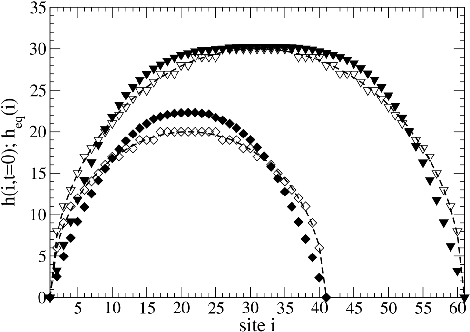
Figure 1: Initial, $h(i,t=0)$, (open symbols) and PD equilibrium, $h_{eq}(i)$, (full symbols) positions of curved steps at $k_{B}T/J=3.0$ for $L$= 41 and 61.

We are interested in the value of the characteristic exponent $x$ in the expected power–law for the growth of $G(t)\propto t^{x}$. Using Langevin theory and simulations, $x$ has been found to be 1/4 for fluctuations driven by PD and 1/2 in case of EC rev1 ; rev2 ; bs ; bladux ; eins1 ; sza . The latter result follows from exact arguments as well au .

To determine $x$ from simulation data, one may monitor the effective exponent $x_{eff}$, in its discretized form ps

$$x_{eff}(t,L)=\ln(G(t_{j})/G(t_{j-1}))/\ln(t_{j}/t_{j-1})$$ (6)

with $t=\sqrt{t_{j}t_{j-1}}$, where $t_{j}$ refers to the discrete time scale, measured in MCS/S.

Indeed, after a diffusive–like behavior, $x_{eff}\approx 1$, at very short times bs , the effective exponent is observed to decrease monotonically rather rapidly to about 1/4 for PD, and to about 1/2 for EC, for flat, tilted, and curved steps, as illustrated in Fig. 2. Note that $x_{eff}$ continues to decrease monotonically, approaching eventually zero, due to the fact that $G(t)$ saturates for pinned steps of finite length. Let us denote the time needed to pass through the characteristic value, $c=$ 1/4 or 1/2, by $t_{c}$, i.e. $x_{eff}(t_{c})=c$. That time depends on temperature, slope, curvature, and, perhaps, most interestingly, the length of the step. Actually, we find strong evidence that $t_{c}$, for sufficiently long steps, increases with $L_{a}=L-2$ in form of a power–law, $L_{a}^{\gamma}$, with $\gamma$ being roughly 1.5 for EC and being roughly 0.5 for EC. Steps with up to about 400 sites have been studied. The observed finite–size behavior suggests that $G(t)$ satisfies the simple power–law, $G(t)\propto t^{x}$, asymptotically in time in the thermodynamic limit, $L_{a}\longrightarrow\infty$.

Figure 2: Effective exponent $x_{eff}$ at $k_{B}T/J=3.0$ for PD, for flat (circle), tilted, with slope $s=1$, (square) and curved (diamond) steps, $L=101$, as well as for EC, for flat (triangle up) and tilted, with $s=1$, (triangle down) steps, $L=201$.

The prefactor, $a$, in front of the asymptotic power–law for $G$, i.e. $G(t)=at^{x}$, turns out to depend significantly on temperature and the type of the step,(a)-(c). To our knowledge, $a$ had not been analyzed in previous simulations of step fluctuations. To take into account finite–size effects, we consider the effective prefactor $a_{eff}$

$$a_{eff}(t,L_{a})=G(t)/t^{x}$$ (7)

with $x$= 1/4 for PD and 1/2 for EC. $L_{a}$ is the number of active sites. The effective prefactor is found to have its, in general plateau–like, maximum, $a_{p}(L_{a})$, at the time $t_{c}$, at which the corresponding effective exponent $x_{eff}$ passes through $c$= 1/4, for PD, or 1/2, for EC. The prefactor $a$ = $a_{p}(\infty)$ is then reached for $L_{a},t\longrightarrow\infty$.

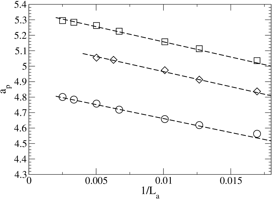
Figure 3: Effective prefactor $a_{p}$ vs. inverse number of active sites $1/L_{a}$ for PD for flat (circle), tilted, with slope $s=1$, (diamond) and curved (square) steps at $k_{B}T/J=3.0$.

$a_{p}(L_{a})$ displays an interesting and simple finite–size behavior, as illustrated, for PD, in Fig. 3. For sufficiently long steps, $a_{p}(L_{a})$ is found to grow, for all types of steps, (a)-(c), like $a_{p}(L_{a})=a_{p}(\infty)-d/L_{a}$, $d$ depending on temperature and on the type of step. Thence, one may easily estimate the prefactor $a(T)$ from the simulation data.

Results of such extrapolations for initially flat steps at various temperatures are shown in Fig. 4. We compare our Monte Carlo findings to predictions of the Langevin theory bew1 ,

$$G(t)=0.46...((k_{B}T)^{3}\Gamma_{h}/\tilde{\beta}^{3}))^{1/4}t^{1/4}$$ (8)

with the step stiffness $\tilde{\beta}$ being

$$\tilde{\beta}=2k_{B}T\sinh^{2}(J/2k_{B}T)$$ (9)

The step mobility $\Gamma_{h}$ follows, apart from a proportionality factor, from the fraction of successful Monte Carlo attempts. In Fig. 4, we fixed this factor by equating the Langevin predictions and the Monte Carlo findings at $k_{B}T/J=1$. Obviously, we observe a very good agrement for the non–trivial temperature dependence of the simulated prefactor $a$ with the prediction based on Langevin theory.

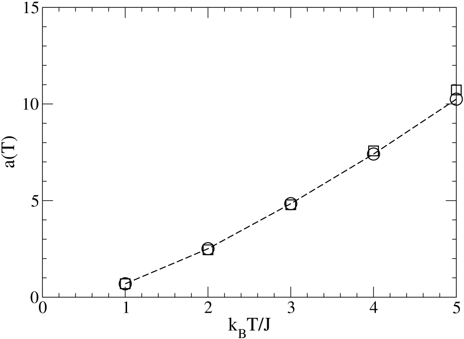
Figure 4: Prefactor $a$ of the step fluctuations for PD, at various temperatures $k_{B}T/J$, comparing Monte Carlo findings (circle), extrapolated to the thermodynamic limit, with predictions based on Langevin theory (square).

It seems worthwhile to note that the prefactor $a$ increases monotonically not only with the temperature but also with the slope of the steps, $a(s)$, see Fig. 5. Consequently, it is significantly larger for curved than for flat steps. Actually, $a$ is observed to depend essentially on the energy of the step. For instance, for tilted steps, we obtained

$$a(s)/a(s=0)\approx E(s)/E(s=0)$$ (10)

where $E(s)$ is the thermal equilibrium energy of steps with the slope $s$.

Because of their pinning at the ends, the steps tend to fluctuate more strongly in the center, as we observed when monitoring the local fluctuations. Of course, this boundary effect is expected to play no role in the limit of indefinitely long steps.

IV Confined steps

We now consider fluctuating, initially flat steps with periphery diffusion, described by the one–dimensional SOS model, Eq.(1), confined by a second step. The confining step is located at distance $d$ from the initial step position $h(i,t=0)=0$, i.e. for all times one has $h(i,t)<d$. A typical Monte Carlo equilibrium configuration for $d=4$ and periphery diffusion is depicted in Fig. 6.

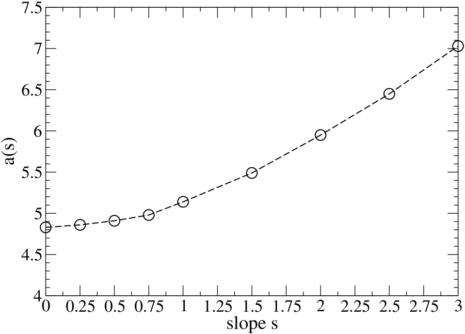
Figure 5: Slope, $s$, dependence of the (extrapolated) prefactor $a$ for tilted steps with PD at $k_{B}T/J=3.0$.

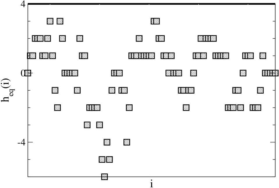
Figure 6: Typical Monte Carlo equilibrium configuration, PD, for a confined step with $d=4$ at $k_{B}T/J=1.0$.

In previous Monte Carlo studies of this toy model deg2 ; deg3 , periodic boundary conditions have been employed, considering PD at fixed temperature, $k_{B}T/J=1.0$, and step length $L=100$. Depending on the separation distance $d$, three different regimes have been identified. For small $d$, $d\leq 3$, the step fluctuations, $G(t)$, have been suggested to grow logarithmically with time. For sufficiently large distances, $d\geq 12$, $G(t)$ is found to behave as for isolated steps, where its power–law like increase is characterised by the exponent $x=1/4$. In the intermediate range of $d$, power–law dependences are observed, with the exponent $x$ being close to 2/11, as may follow from theoretical descriptions for the dynamics of the border ledge of a crystal facet fps ; deg1 . However, deviations from the simple power–law have been found to occur, possibly, due to, for instance, crossover effects related to the separation distance $d$ deg2 ; deg3 ; ep . No simulations had been done for EC, where scaling arguments and Langevin theory fps ; deg1 may suggest $x$= 2/5, instead of 1/2 as for isolated steps.

The aim of the present Monte Carlo study is to study the toy model in more detail, investigating, among others, finite–size effects, the deviations from simple-power laws and the long–time behavior of $G(t)$. Mostly, we employed pinned boundary conditions.

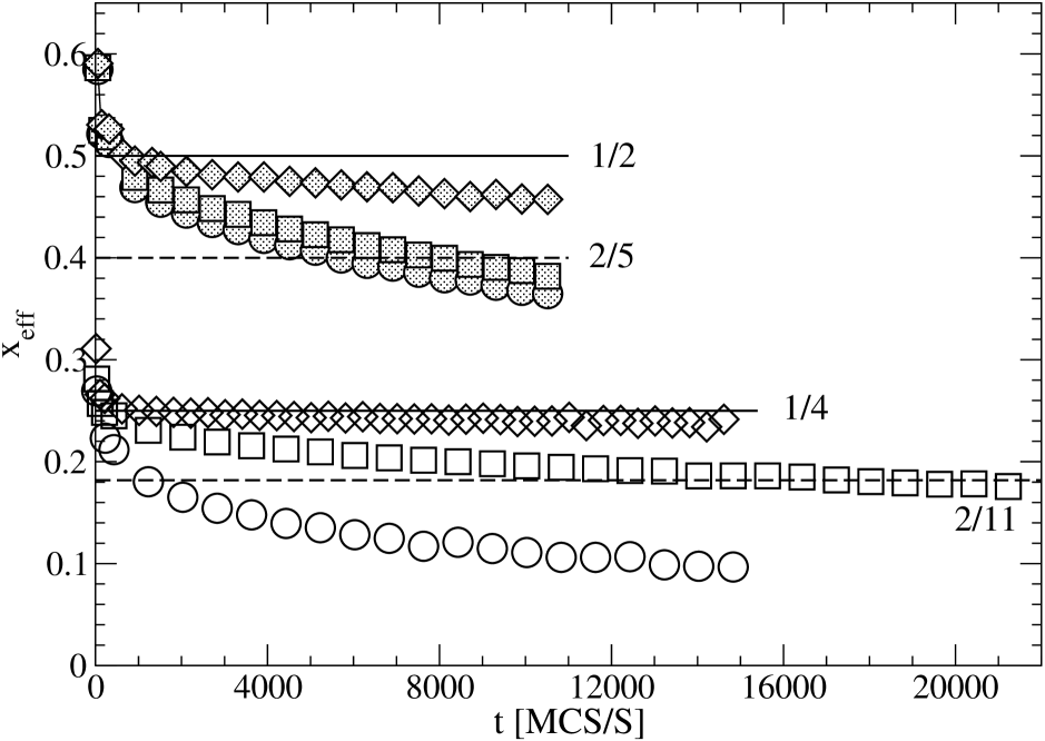
Figure 7: Effective exponent $x_{eff}$ for confined steps of length $L=201$, with PD (open symbols) at $k_{B}T/J=1.0$, for $d$= 3 (circle), 5 (square), and 16 (diamond), and with EC (shaded symbols) at $k_{B}T/J=3.0$, for $d=3$ (circle), 20 (square), and 300 (diamond).

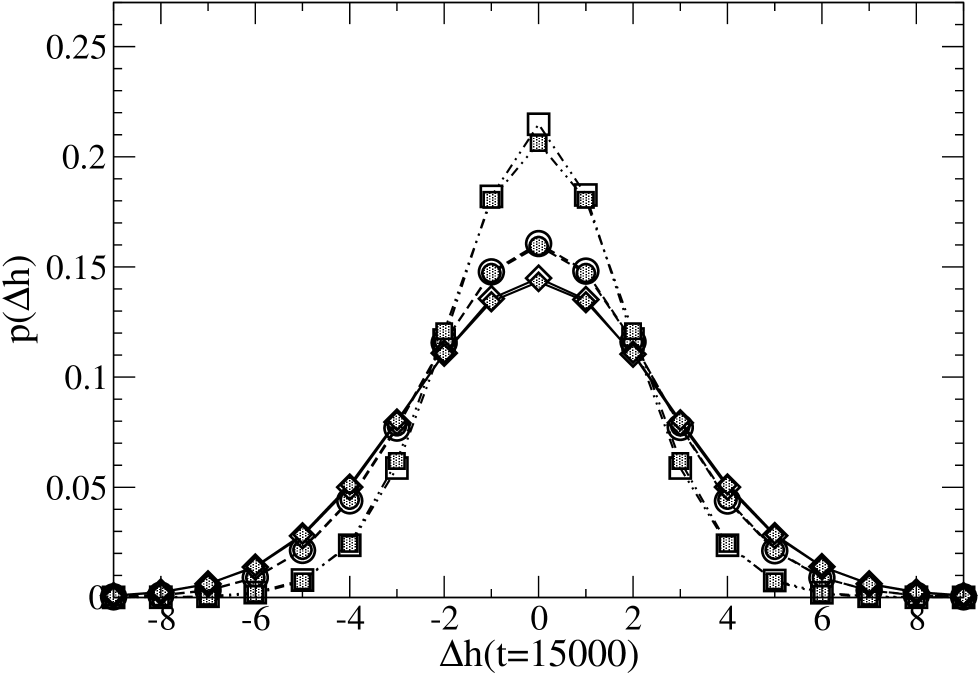
Figure 8: Histograms of $(\Delta h)$ for pinned isolated (diamond) and confined steps with $d=3$ (square) and 5 (circle) of length $L=201$ at $k_{B}T/J=1.0$, using PD, comparing simulation data (open symbols) at $t=15000$ MCS/S to Gaussian distributions (shaded symbols) with the standard deviation set equal to the fluctuation length.

Let us first deal with PD. In particular, we monitored the dependence of the effective exponent $x_{eff}(t)$ on step length, temperature, and separation distance. At first sight, one may distinguish three regimes, (i)-(iii), see below, following and generalizing the previous analysis deg2 . Examples are depicted in Fig. 7.

In all cases, at very early times, $G(t)$ exhibits, as for isolated steps, a diffusive–like behavior due to independent moves at randomly chosen sites, with $x_{eff}$ near one. A much finer time resolution than the one shown in Fig. 7, would be needed to demonstrate that behavior. Because of the step stiffness, the growth of the fluctuations then slows down bs , with $x_{eff}$ decreasing more gradually and, always, monotonically. Now, (i) the effective exponent may approach rather quickly zero, without any striking anomalies. This may happen when the steps are rather short, independent of $d$, because $G(t)$ saturates quite soon. This rather trivial effect is not displayed in Fig. 7. It may also also happen for longer steps and fairly small $d$, as depicted in Fig. 7, possibly, due to the suggested logarithmic rise of $G(t)$ deg2 ; deg3 . On the other hand, (ii) for sufficiently large values of $d$, $G(t)$ seems to grow as for isolated steps, with $x_{eff}$ being, in quite extended time intervals, close to 1/4. The most interesting case is encountered for the intermediate regime (iii), where, again for quite extended time intervals, one observes a power–law like behavior, with $x_{eff}$ being close to 2/11. Certainly, for a more quantitative description, temperature will play an important role as well, as will be discussed below.

Clearly, in general, $G(t)$ is expected to be, asymptotically, finite, in all three regimes of the toy model, with the corresponding fluctuation length $g(t)=\sqrt{G(t)}$ being bounded by the distance $d$. In any event, it is of much interest to clarify the conditions, under which one may observe typical features of the three regimes (i)-(iii).

We checked, in regime (i), whether there is evidence of the logarithmic growth of $G(t)$, which had been suggested to occur, as in a step train, for small $d$ rev1 ; deg2 ; deg3 . We assumed the form $G(t)=b\ln(t)$ and monitored the effective prefactor $b=b(t)$. In fact, for instance, for $d=3$ at $k_{B}T/J$= 1.0 and $L=201$, see Fig. 7, the prefactor is found to be nearly constant in a quite large time range, measured in MCS/S, $5000\lesssim t\lesssim 25000$. Eventually, it starts to decrease, due to finite–size saturation of the fluctuations.

The time window increases with the length of the steps. We tend to conclude that the fluctuations satisfy, over a fairly large time interval, the logarithmic growth law. We note in passing that there is no indication of logarithmic behavior for small steps, where $x_{eff}$ goes quickly to zero caused by the fast saturation of $G(t)$. At higher temperatures, regime(i) extends to a larger range of separation distances $d$, as will be explained below.

Obviously, in regime (ii), where $x_{eff}\approx 1/4$, the fluctuation length of isolated steps has to be small compared to the separation distance $d$. For sufficiently long steps, it may happen in large time windows, see Fig. 7, but asymptotically, $L,t\longrightarrow\infty$, the growth of $G(t)$ will be ultimately limited by $d$.

In the, perhaps, most interesting regime of moderate distances $d$, regime (iii), we observe, again in intermediate time intervals, a power–law like behavior of $G(t)$, with exponent close to 2/11 for PD, as illustrated in Fig. 7. The value has been argued to reflect the long–range interactions of the fluctuating step with another step or an ensemble of other steps ep . Indeed, in the toy model, the entropic repulsion with the straight step may cause such an interaction, tending to hinder the growth of the fluctuations and tending to reduce the value of the characteristic exponent, from 1/4 to 2/11.

Before discussing the range of validity of this regime, it seems useful to monitor and analyze the fluctuation length $g(t)$ in more detail. Actually, $g$ is found to be related to the standard deviation of the histograms $p(\Delta h)(t)$, describing the probability that the step position differs, after time $t+t_{0}$, from its equilibrium value, at $t_{0}$, by $\Delta h$. More concretely,

$$\Delta h=\sum_{i}(h(i,t+t_{0})-h(i,t_{0}))/L_{a}$$ (11)

averaging over all active step sites $i$. Typical results are depicted in Fig. 8 at $k_{B}T=1.0$ and $L=201$, for different values of $d$ as well as for isolated steps. The simulation data are compared to the Gaussian probability distribution with the standard deviation $\sigma$ set equal to the fluctuation length $g(t)$. As seen from the figure, there is a very good agreement, with a very slight asymmetry in the simulation histogram for small $d$, as expected due to the presence of the confining step. It is worthwhile mentioning that similar observations hold in general, including periodic boundary conditions as well.

The criterion for encountering the unconventional effective exponent, $x_{eff}\approx 2/11$, may be argued to be that, for sufficiently long steps, the fluctuation length $g_{iso}$ of the corresponding isolated step is just somewhat smaller than $d$, so that the entropic repulsion is strong enough to change the unconstrained fluctuations of isolated steps to those reflecting the presence of the second step. If the fluctuation length is too small, or if $d$ is too large, then one is in the regime of the fluctuations of isolated steps, (ii). In the opposite case, regime (i), remainders of the logarithmic growth are seen. Following this consideration, the extent of regime (iii) depends, especially, on temperature.

A few typical examples are: At $k_{B}T/J=1.0$ and $L$ being about 100 to 200, $g_{iso}$ is, for $t$ ranging from 5000 to 20000 MCS/S, in between 2.5 and 2.7, increasing with $t$. At $k_{B}T/J=3.0$, $g_{iso}$ rises, in the same time window, from about 6.3 to about 7.5. Accordingly, the regime (iii), where $x_{eff}$ is, in a rather long time interval, near 2/11, is expected to shift to larger distances $d$ at the higher temperature. We checked the suggestion by varying $d=$ from 5 to 15, at $k_{B}T/J=3.0$. Now, the unconventional exponent, 2/11, is, indeed, found to be quite pronounced at $d$ around 10. Thence, analysis of the correlation length for isolated steps will lead to reasonable choices of separation distances to encounter the unconventional growth in the fluctuations of confined steps.

As has been argued above, the power–law behavior of $G(t)$ with the exponent 2/11 is not expected to occur asymptotically, $t,L\longrightarrow\infty$, in the toy model for finite distance $d$, because $G(t)$ will be limited by $d$, in contrast to the situation for isolated steps. The effective exponent, after having displayed a plateau–like behavior near 2/11, continues to decrease monotonically, until it finally reaches zero. Actually, we monitored, at fixed $d$, the time needed to reach the, supposedly, characteristic value of $x_{eff}=2/11$, i.e., $t_{2/11}$, as a function of step length $L$. As had been mentioned above, the corresponding time $t_{1/4}$ for isolated steps is found to diverge as $L$ is going to infinity, showing that $G(t)$ obeys, in the thermodynamic limit, a simple power–law asymptotically in time. Now, for confined steps, the simple power–law describes only a transient behavior. As shown in Fig. 9, for $d=4$ and 5, we obtain, to a good degree of accuracy, for sufficiently long steps $t_{2/11}(L_{a})=t_{\infty}-c/L_{a}$, with a finite $t_{\infty}$, reflecting the saturation of $G(t)$ at finite time due to the presence of the second step in the toy model.

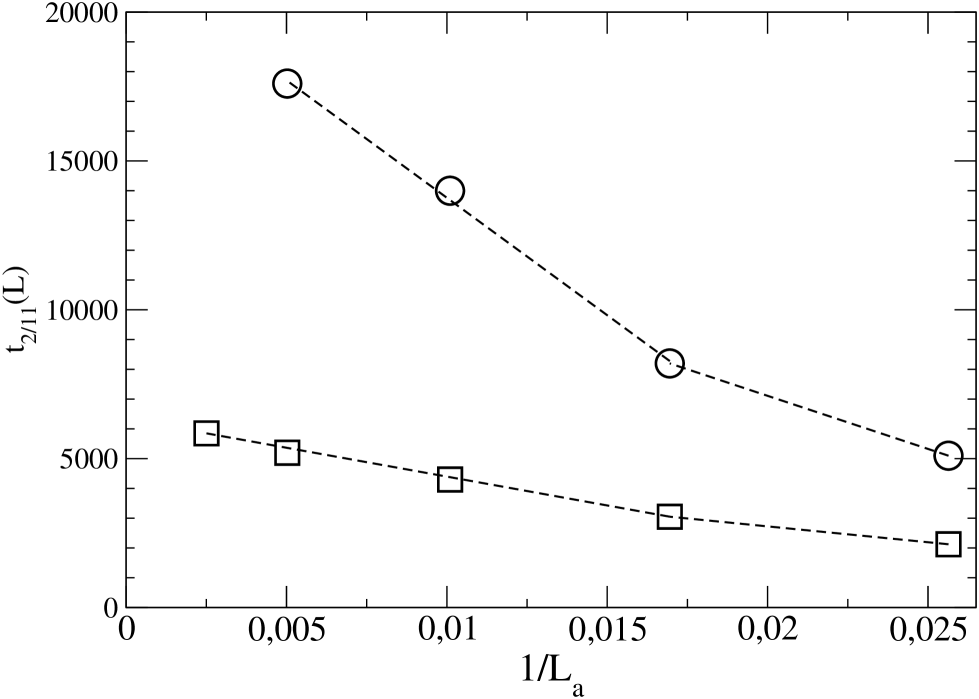
Figure 9: Finite–size dependence of characteristic time $t_{2/11}$ for confined steps with PD for $d=4$ (square) and $d=5$ (circle) at $k_{B}T/J=1.0$.

To observe, possibly, the characteristic value of 2/11 in the asymptotic limit, the second step may be placed at indefinite distance from the fluctuating step, with true, physical long–range interactions between the two steps. Limits had to be taken in the appropriate order. Note that at larger distances, $d$, longer and longer runs would be needed to determine the limiting size–dependence, and we refrained from attempting to do it.

For EC, the positions of the fluctuating step tend to be repelled due the entropic repulsion exerted by the straight step. Thence, in thermal equilibrium, for pinned boundary conditions, $h_{eq}(i)$ takes a curved form, somewhat similar to the one shown in Fig. 1. The maximal height of the equilibrium shape, at given temperature and step length, increases with decreasing $d$. For instance, for steps of length $L_{a}$= 199 at $k_{B}T/J=3.0$, as depicted in Fig. 7, the maximal height increases from about 17 to about 33, when lowering $d$ from 20 to 3. Then, already for small distances $d$, as depicted in Fig. 7 for $d=3$, the effective exponent $x_{eff}$ does not fall off quickly, unlike in regime (i) for PD, with $G(t)$ growing faster than logarithmically in the time span we studied. As shown in Fig. 7 as well, for moderate $d$, $d=20$, there seems to exist a time range in which $G(t)$ displays a power–law like behavior with the effective exponent being close to 2/5, as had been predicted for the border ledge of a crystal facet fps ; deg1 .

To avoid complications resulting from the curved equilibrium shape of the step positions, for EC, one may modify the toy model by introducing another straight step, placed, symmetrically, at distance $-d$ from the fluctuating step. For this variant, $x_{eff}$ exhibits similar features as those shown in Fig. 7, adjusting the separation distance between the fluctuating and straight steps. In any event, the EC case with confinement may deserve further attention. Perhaps, analytical calculations on the toy models would be feasible. They would be most welcome.

V Summary

We studied thermal fluctuations, $G(t)$, of isolated and confined steps of monatomic height on low–index crystal surfaces in the framework of one–dimensional SOS models. Periphery diffusion, PD, and evaporation–condensation, EC, have been analyzed, using Monte Carlo techniques.

For isolated steps, we found that $G(t)$ grows asymptotically, i.e. for $t\longrightarrow\infty$, in the limit of indefinitely many step sites, as $G(t)=at^{x}$. In the case of PD, the characteristic exponent $x$ is observed to be 1/4, independent of slope and curvature as well as temperature of the steps. The prefactor $a$, on the other hand, varies with the geometry and temperature, being determined by the energy of the step. The temperature dependence for initially flat steps agrees well with the one predicted by Langevin theory. In the case of EC, the exponent $x$ is found to be 1/2, independent of slope and temperature.

For confined steps, we considered, following previous simulations, a toy model with an initially flat, fluctuating step in the presence of a second fixed, straight step, at initial distance $d$. We mainly studied PD. For rather large steps, we find, depending on $d$, three different regimes, where $G(t)$ shows, for quite extended time intervals, either a power–law like behavior or logarithmic growth.

The power–law like behavior may be due to unconstrained fluctuations as for isolated steps, with $x_{eff}$ close to 1/4 or due to fluctuations hindered by the entropic repulsion of the confining step, with $x_{eff}$ being near 2/11. In all cases, fluctuations are found to satisfy a Gaussian distribution. Comparison of the standard deviation (or fluctuation length) of the isolated steps to the separation distance provides the clue to determine the range of validity of the various regimes with logarithmic or power–law like growth of $G(t)$. Eventually, $G(t)$ will be limited by $d$, so that asymptotically, $t,L\longrightarrow\infty$, the effective exponent $x_{eff}$ will approach zero, for all finite values of $d$.

In case of EC, the effective exponent, due to entropic repulsion, may be expected to be 2/5, as predicted by related scaling arguments and Langevin theory. Indeed, a related power–law like growth of the step fluctuations seems to occur for suitable choices of distance $d$, temperature, and step length. However, the simulations of the toy model are strongly affected by the fact that the average step position is not conserved for EC. Further studies are desired for clarification.

- (1) H–C. Jeong and E. D. Williams, Surf. Sci. Rep. 34, 175 (1999).
- (2) M. Giesen, Prog. Surf. Sci. 68, 1 (2001).
- (3) C. Misbah, O. Pierre-Louis, and Y. Saito, Rev. Mod. Phys. 82, 981 (2010).
- (4) P. L. Ferrari, M. Prähofer, and H. Spohn, Phys. Rev. E 69, 035102 (2004).
- (5) A. Pimpinelli, M. Degawa, T. L. Einstein, and E. D. Williams, Surf. Sci. Lett. 598, L355 (2005).
- (6) M. Degawa, T. J. Stasevich, W. G. Cullen, A. Pimpinelli, T. L. Einstein, and E. D. Williams, Phys. Rev. Lett. 97, 080601 (2006).
- (7) M. Degawa, T. J. Stasevich, A. Pimpinelli, T. L. Einstein, and E. D. Williams, Surf. Sci. 601, 3979 (2007).
- (8) E. E. Gruber and W. W. Mullins, J. Phys. Chem. Solids 28, 875 (1967).
- (9) M. E. Fisher and D. S. Fisher, Phys. Rev. B 25, 3192 (1982).
- (10) T. L. Einstein and A. Pimpinelli, arXiv: 1312.4910; J. Stat. Phys.(2014) (DOI) 10.1007/s10955-014-0981-3.
- (11) D. P. Landau and K. Binder, A Guide to Monte Carlo Simulations in Statistical Physics (University Press, Cambridge, 2005).
- (12) M. Pleimling and W. Selke, Eur. Phys. J. B 1 385 (1998).
- (13) M. Bisani and W. Selke, Surf. Sci. 437, 137 (1999).
- (14) W. Blagojevic and P. M. Duxbury, in Dynamics of crystal surfaces and interfaces. ed. by P. M. Duxbury and T. J. Pence (Plenum Press, New York, London, 1997), p.1.
- (15) S. V. Khare and T. L. Einstein, Phys. Rev. B 57, 4782 (1998).
- (16) F. Szalma, W. Selke, and S. Fischer, Physica A 294, 313 (2001).
- (17) D. B. Abraham and P. J. Upton, Phys. Rev. B 39, 736 (1989).
- (18) N. C. Bartelt, T. L. Einstein, and E. D. Williams, Surf. Sci. 276, 308 (1992).