NLTE 1.5D Modeling of Red Giant Stars

Abstract

Spectra for 2D stars in the 1.5D approximation are created from synthetic spectra of 1D non-local thermodynamic equilibrium (NLTE) spherical model atmospheres produced by the PHOENIX code. The 1.5D stars have the spatially averaged Rayleigh-Jeans flux of a K3-4 III star, while varying the temperature difference between the two 1D component models ($\Delta T_{\mathrm{1.5D}}$), and the relative surface area covered. Synthetic observable quantities from the 1.5D stars are fitted with quantities from NLTE and local thermodynamic equilibrium (LTE) 1D models to assess the errors in inferred $T_{\mathrm{eff}}$ values from assuming horizontal homogeneity and LTE. Five different quantities are fit to determine the $T_{\mathrm{eff}}$ of the 1.5D stars: UBVRI photometric colors, absolute surface flux SEDs, relative SEDs, continuum normalized spectra, and TiO band profiles. In all cases except the TiO band profiles, the inferred $T_{\mathrm{eff}}$ value increases with increasing $\Delta T_{\mathrm{1.5D}}$. In all cases, the inferred $T_{\mathrm{eff}}$ value from fitting 1D LTE quantities is higher than from fitting 1D NLTE quantities and is approximately constant as a function of $\Delta T_{\mathrm{1.5D}}$ within each case. The difference between LTE and NLTE for the TiO bands is caused indirectly by the NLTE temperature structure of the upper atmosphere, as the bands are computed in LTE. We conclude that the difference between $T_{\mathrm{eff}}$ values derived from NLTE and LTE modelling is relatively insensitive to the degree of the horizontal inhomogeneity of the star being modeled, and largely depends on the observable quantity being fit.

1 INTRODUCTION

1.1 Red Giant Stars

Red giant stars rank among the brightest stars in the Galaxy, being generally much brighter in the visible band than main sequence stars of the same spectral type. But this only partially accounts for their brightness as large portion of their flux is emitted in the near-IR. This, combined with their enormous surface areas, gives them such large luminosities that they are easily observable even in very remote stellar populations. Red giants grant us a tool for probing nearly all regions of the Galaxy using a common indicator, a feat unparalleled by most other types of stars.

Because many red giants are low to intermediate mass stars that have evolved beyond the main sequence, generally found in older stellar populations, their abundances can be indicators of early Galactic chemical evolution. For example, by comparing observations of Galactic bulge giants with those of giants located in the thin and thick disks and halo, it has been shown that the bulge likely experienced similar formation timescales, chemical evolution histories, star formation rates and initial mass functions as the local thick disk population (Meléndez et al., 2008; Alves-Brito et al., 2010). Bulge and disk giants show some differences in their chemical abundances, with the bulge giants showing a higher relative abundance of select elements than the disk giants, suggesting more rapid chemical enrichment, possibly by ejecta from supernovae of Types Ia and II (Cunha & Smith, 2006). Observations of red clump giants in the bulge have also produced additional evidence of a central bar (Stanek et al., 1997), with their apparent visual magnitudes being brighter at some Galactic latitudes than others.

The tip of the red giant branch (TRGB) can also be used as a standard candle to determine distances to nearby galaxies. The distance moduli obtained from the $I$ pass-band magnitude of the TRGB are comparable with those from primary distance indicators like Cepheids and RR Lyraes (Makarov et al., 2006), and in some cases even suggest a reevaluation of the metallicity dependence and zero point calibration of the Cepheid distance scale (Salaris & Cassisi, 1998; Rizzi et al., 2007). The TRGB method even has advantages over other distance determinations like those of Cepheids and RR Lyraes: $\left(1\right)$ the TRGB method requires much less telescope time than variable stars; $\left(2\right)$ the $I$ magnitude of the TRGB is insensitive to the variation of metallicity for $\mathrm{[Fe/H]}<-$ 0.7; and $\left(3\right)$ the TRGB suffers less from extinction problems than Cepheids, which are in general located in star-forming regions (Lee et al., 1993).

1.2 Modeling Stellar Atmospheres

Much of what is now known about all types of stars comes from fitting the predicted quantities from atmospheric models to observations. Estimates of the solar chemical abundances come from fitting synthetic spectral line profiles and equivalent widths to those observed in the Sun (Ross & Aller, 1976; Asplund et al., 2009; Caffau et al., 2011). Calibrations of stellar parameters, such as $g$, $M_{V}$, $T_{\mathrm{eff}}$, $L$, and $R_{0}$, for different spectral types are found from fitting models (Martins et al., 2005). Beyond studying single stars, model atmospheres can be used to determine qualities of larger structures as well. The age-metallicity and color-metallicity relations of globular clusters can be determined from the abundances of individual red giants within the clusters (Pilachowski et al., 1983; Carretta & Gratton, 1997; Carretta et al., 2010).

In this work, we will explore the limitations of two of the simplifying assumptions of atmospheric modeling: horizontal homogeneity and local thermodynamic equilibrium (LTE). Both of these assumptions have been generally adopted because they are more computationally practical than the alternatives, requiring less time and fewer resources to arrive at a result. By comparison, horizontal inhomogeneity requires model atmospheres to be calculated in two or three geometric dimensions (2D or 3D models) instead of just one, and non-LTE (NLTE) requires that each level population be computed in statistical equilibrium (SE) using iterative processes.

However, horizontal homogeneity and LTE both limit how realistic a model can be. Simulations of red giant atmospheres performed in 3D have confirmed that turbulent surface convection causes horizontal inhomogeneities to form (Collet et al., 2007; Kučinskas et al., 2013b), such as visually observable surface features like solar granulation (Mathur et al., 2011; Tremblay et al., 2013). These features are known to lead to detectable effects, such as altering predicted line strengths and shapes and, thus, inferred elemental abundances (Collet et al., 2008, 2009; Dobrovolskas et al., 2013; Hayek et al., 2011; Kučinskas et al., 2013a; Mashonkina et al., 2013). For 3D models of red giant atmospheres, whose modeling parameters span the ranges of 3600 K $\leq T_{\mathrm{eff}}\leq$ 5200 K, 1.0 $\leq\mathrm{log\,}g\leq$ 3.0, and -3.0 $\leq\mathrm{[Fe/H]}\leq$ 0.0, granules have been shown to span a range of sizes from as small as on the order of 10⁸ cm to as large as 2 $\times$ 10¹² cm, with the majority on the order of 10¹¹ cm (Collet et al., 2007; Chiavassa et al., 2010; Hayek et al., 2011; Ludwig & Kučinskas, 2012; Magic et al., 2013b; Tremblay et al., 2013). The cooler stars and stars with lower values of $\mathrm{log}\,g$ generally display larger features. For the same set of 3D models, the root mean square (RMS) temperature variation among these features at optical depth unity is usually in the range of $\sim$ 2 to 5 $\%$, or $\sim$ 200 to 300 K for the parameters listed above, although variations can reach 2000 K between the hottest and coolest areas (Collet et al., 2008, 2009; Kučinskas et al., 2013a, b; Ludwig & Kučinskas, 2012; Magic et al., 2013a, b; Samadi et al., 2013; Tremblay et al., 2013). Most of the 3D models reported in the literature have $T_{\mathrm{eff}}$ $\approx$ 4500 K, with $\Delta T$ varying by $\sim$ 200 K.

For stars exhibiting horizontal inhomogeneities, where the temperature varies across the features, $T_{\mathrm{eff}}$ is no longer a well defined quantity. By definition, $T_{\mathrm{eff}}$ is derived from the Stefan-Boltzmann law, where the bolometric luminosity ($L_{\mathrm{bol}}$) of a star is proportional to the fourth power of its $T_{\mathrm{eff}}$ ($T_{\mathrm{eff,S-B}}$). The $T_{\mathrm{eff,S-B}}$ of a horizontally inhomogeneous star may be similarly found by summing the $L_{\mathrm{bol}}$ of each of the inhomogeneous components, weighted by their relative surface coverage, and taking the fourth root of the result. This quantity is defined empirically by intrinsic properties of real or model stars and is independent of fitting models to observable quantities. Alternatively, another model fitting independent $T_{\mathrm{eff}}$ can be defined from the long wavelength tails of stellar spectra. Because flux has a linear dependence on $T_{\mathrm{eff}}$ in the Rayleigh-Jeans limit, an estimate of the $T_{\mathrm{eff}}$ can be made from measuring the absolute surface flux of the R-J tail. This dependence is used by the Infrared Flux Method (Ramírez & Meléndez, 2005) to determine $T_{\mathrm{eff}}$ from the R-J tails of spectra ($T_{\mathrm{eff,R-J}}$).

The key idea for a horizontally inhomogeneous star having the same $T_{\mathrm{eff,S-B}}$ as a horizontally homogeneous star, is that the SEDs will differ based on the variation of the modeling parameters, such as $T_{\mathrm{eff}}$, across the inhomogeneous surface. For example, using the Planck function,

$$B_{\lambda}(T_{\mathrm{eff}})=\frac{2hc^{2}}{\lambda^{5}}\left(e^{hc/\lambda k_{B}T_{\mathrm{eff}}}-1\right)^{-1},$$ (1)

to describe the shape of a stellar continuum illustrates the issue directly (Uitenbroek & Criscuoli, 2011). A star with a range of differing temperatures across the surface does not have a directly obvious value of $T_{\mathrm{eff}}$ that should be used, and because of the equation’s non-linear dependence on $T_{\mathrm{eff}}$, this is an important question. The higher temperature material will contribute disproportionately more flux than the lower temperature material, with a dependence on wavelength, and will alter the spectrum from that of a horizontally homogeneous star of the same $T_{\mathrm{eff,S-B}}$ accordingly.

The most noticeable departure of LTE models from observed stars comes from comparing computed and observed spectral features and SEDs. For 1D models of red giants, NLTE models have been shown to be more accurate than LTE models in predicting the overall monochromatic flux ($F_{\lambda}$) levels of SEDs and strengths of individual spectral lines, with the notable exceptions of molecular absorption bands and the near-UV band flux (Short & Hauschildt, 2003, 2006, 2009; Bergemann et al., 2013). Calculating the molecular level populations in NLTE is computationally demanding, and is not handled in many atmospheric modeling codes. Both LTE and NLTE models over-predict the near-UV $F_{\lambda}$ levels of cool red giants. In the case of the near-UV $F_{\lambda}$ levels, NLTE models are worse in the over-prediction than their LTE counterparts. The NLTE effects of Fe group elements on the model structure and $F_{\lambda}$ distribution have been shown to be much more important for predicting a SED than the NLTE effects of all the light metals combined, and serve to substantially increase the near-UV $F_{\lambda}$ levels as a result of NLTE Fe I overionization (Short & Hauschildt, 2009). The magnitude of this effect has been shown to be inversely proportional to the completeness of the Fe I atomic model used in the atmospheric modeling (Mashonkina et al., 2011), discussed in detail in Section 2.1. These failures of 1D NLTE models to predict observable quantities may be, in part, related to the exclusion of horizontal inhomogeneities in the models.

1.3 Present Work

Our primary goal is investigating the relation between errors introduced in determining a star’s $T_{\mathrm{eff}}$ from assuming horizontal homogeneity and those introduced by assuming LTE. We look to determine how distinguishable 3D hydro and NLTE effects are when looking at low resolution diagnostics (photometric colors and overall SEDs). The error inherent in assuming LTE is expected to remain approximately constant for different levels of horizontal inhomogeneity, as any changes in a LTE spectrum caused by the inhomogeneities should also be represented to a similar degree in the corresponding NLTE spectrum, as the relative difference in the flux distribution between LTE and NLTE should remain roughly constant within the $T_{\mathrm{eff}}$ range studied in this work.

Section 2 outlines the parameters used for the 1D NLTE and LTE model grids, and the methods used in creating and processing the 1.5D NLTE spectra. Section 3 presents the results of fitting 1D SEDs and spectra to the 1.5D SEDs and spectra. Section 4 gives a brief summary and discussion of the results.

2 1D AND 1.5D ATMOSPHERIC MODELS

In general, the calculation of a 2D model atmosphere requires a very substantial increase in computational effort over that needed for 1D models. However, there are two regimes of validity for which the situation simplifies; these are often referred to as 1.5D models. The valid regimes are either 1) when the geometric scale of the inhomogeneities is so small that they are very optically thin, and every emergent ray may be assumed to have fully sampled both warm and cool components of the atmosphere many times, or 2) that the inhomogeneities are large enough that they are optically thick to their own radiation so that the flux is similar to that of two spatially unresolved stars. Regardless, both regimes require that the inhomogeneities be small enough and randomly distributed so that there is no correlation between component $T_{\mathrm{eff}}$ values and limb darkening. By assuming the average size of surface features to be that of 3D hydro modeled red giant granules, we satisfy both conditions of the larger inhomogeneity regime.

We construct our 1.5D SEDs by taking the linear average of two 1D NLTE SEDs. Two-dimensional information, such as the difference in temperature among features or the relative portion of the stellar surface covered by the different features, can be approximated by choosing the parameters of the 1D components being averaged, and the averaging weights. These 1.5D NLTE SEDs and derived colors, approximating 2D effects, are treated as artificial “observations” of real stars that are fitted with a library of NLTE and LTE 1D trial spectra for inferring the $T_{\mathrm{eff}}$ of the 1.5D stars. A grid of 50 1D stellar model atmospheres and corresponding synthetic spectra was produced for this purpose using the PHOENIX code.

2.1 PHOENIX

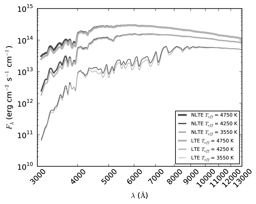
Figure 1: PHOENIX LTE and NLTE synthetic spectra generated from the hottest and coolest grid models and the 1D model with the same $T_{\mathrm{eff,R-J}}$ (see Section 1.2 as the 1.5D spectra. The high resolution spectra generated by PHOENIX were convolved with a FWHM = 50 Å Gaussian kernel, and the resultant spectra are displayed. The LTE spectra with $T_{\mathrm{eff}}$ = 4250 K and 4750 K are mostly hidden behind their NLTE counterparts.

The PHOENIX code can be used to model NLTE atmospheres and spectra of stellar objects throughout the H-R diagram (Baron & Hauschildt, 1998; Hauschildt et al., 1997; Brott & Hauschildt, 2005). PHOENIX version 15 is utilized for all modeling calculations in this work. It is important to include NLTE effects in model atmospheres and synthetic spectra. Together, they can lead to a difference in the blue and near-UV bands flux of up to 50% over corresponding PHOENIX LTE models of red giant stars as a result of NLTE Fe I overionization (Short & Hauschildt, 2003, 2009), displayed in Fig. 1. It is also understood that NLTE radiative equilibrium in these stars is model-dependent and is known to depend on the completeness of the atomic model of Fe I and the completeness and accuracy of the collisional cross-sections for Fe I ionization. While the free electron collisional cross-sections for Fe I used by PHOENIX are robust, it does not take into account H collisions, and it has been cautioned that this may cause PHOENIX to overestimate the effects of Fe I overionization (Asplund, 2005). Additionally, it was shown by Mashonkina et al. (2011) that using a more complete Fe I atomic model than that used by PHOENIX will reduce overionization effects by providing more Fe I high energy excited states to facilitate recombinations from Fe II. They also found that the greater the number of energy levels within $\Delta E$ = k$T_{\mathrm{eff}}$ of the ground state ionization energy ($\chi_{\mathrm{ion}}$), the more accurate the NLTE ionization equilibrium solution. The number of energy levels in our model Fe I atom within $\Delta E$ = k$T_{\mathrm{eff}}$ of $\chi_{\mathrm{ion}}$ ranges from one to four as $T_{\mathrm{eff}}$ increases from 4250 ($T_{\mathrm{eff,R-J}}$ of our 1.5D spectra) to 4750 K (our hottest 1.5D component). This has been found to be too few to accurately compute the NLTE recombination rate, and we expect to over-estimate the NLTE Fe I overionization. However, we note that the 1.5D ’target’ spectra and the 1D library of fitted NLTE spectra were computed with the same Fe I atomic model. Therefore, we expect the difference between fitted 1D NLTE $T_{\mathrm{eff}}$ values and $T_{\mathrm{eff,S-B}}$ to be dominated by horizontal inhomogeneity effects. We also note that the magnitude of any difference in inferred $T_{\mathrm{eff}}$ value between fitting with 1D NLTE spectra and 1D LTE spectra will be over estimated, especially for any diagnostics involving wavebands bluer than the V filter, where the overionization effects are dominant. Therefore we concern ourselves primarily with how this difference depends on the degree of inhomogeneity in the 1.5D spectra being fit, and ignore the magnitude.

The stellar parameters adopted for our $T_{\mathrm{eff,R-J}}$ equivalent 1D star are $T_{\mathrm{eff}}$ = 4250 K, log $g$ = 2.0, and [M/H] = -0.5 with the alpha elements, from O to Ti, enhanced by [A/H] = +0.3 dex. The NLTE models were constructed by treating the 20 atomic species listed in Table 1 as NLTE species when calculating energy level populations, all of them in the neutral state and most in the singly ionized state as well (Short & Hauschildt, 2005). PHOENIX does not calculate level populations for molecular species in NLTE; molecules are treated in LTE for NLTE models and spectra.

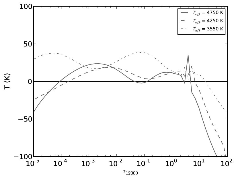
Figure 2: $T_{\mathrm{NLTE}}$($\tau$) – $T_{\mathrm{LTE}}$($\tau$) for PHOENIX atmospheric models as functions of the monochromatic continuum optical depth at 12000 Å representing the same three models as in Fig. 1.

NLTE radiative equilibrium is complex in that any given transition may either heat or cool the atmosphere with respect to LTE, depending on how rapidly $\tau_{\lambda}$ increases inward at the transition wavelength, whether the transition is located in the Wien or Rayleigh-Jeans regime, and whether the transition is a net heater or cooler in LTE with respect to the gray atmosphere (Short et al., 2012). For our $T_{\mathrm{eff}}$ range , all of the NLTE models exhibit a surface cooling effect in the outermost layers of the atmosphere. This is displayed in Fig. 2 as a lower temperature in the NLTE models than in the LTE ones for a given $\tau_{12000}$. For the majority of the upper atmosphere, between $\tau_{12000}\approx$ 10^-4 and 10^-1, the opposite is seen, with the NLTE models having a higher temperature than the LTE ones.

To prepare the grid of models, we varied the $T_{\mathrm{eff}}$ value from 3550 K to 4750 K, with $\Delta T_{\mathrm{eff}}$ = 50 K, and produced both LTE and NLTE models. Upon convergence of a model structure, two different spectra were synthesized for each model, the fully line blanketed SED and the pure continuum SED for use in normalizing the flux in the line blanketed SEDs. This calculation is always performed in LTE even when synthesizing the continuum of a NLTE model because PHOENIX cannot omit the NLTE b-b transitions in the calculations when synthesizing a spectrum. In all spectral synthesis cases, the SEDs are sampled from $\lambda$ = 3000 to 13000 Å as shown in Table 2, with variable spacings, $\Delta\lambda$, to approximately preserve the spectral resolution, $R=\lambda/\Delta\lambda$, across the full range at $R\approx$ 300000 to 400000. In addition to this, the NLTE SEDs are sampled at supplementary points that ensure each NLTE spectral line is critically sampled; these points are automatically distributed over each line by PHOENIX.

Finally, to increase the apparent formal numerical resolution of the grid’s $T_{\mathrm{eff}}$ range sampling, additional SEDs were linearly interpolated between neighboring SEDs in the grid to reach a final apparent temperature resolution of 25 K. This was done to smooth the final fitted $T_{\mathrm{eff}}$ value versus degree of inhomogeneity relation. However, we note that this does not decrease the formal uncertainty of the $T_{\mathrm{eff}}$ determination. Linear interpolation of the flux values was used instead of interpolating the log flux values because at the small ratio of $\Delta T_{\mathrm{eff}}/T_{\mathrm{eff}}$, the relative difference of the monochromatic flux ($\Delta F_{\lambda}/F_{\lambda}$) between the two methods was less than 1.0 % at all wavelength sampling points.

2.2 1.5D SED generation, post-processing, and analysis

Seventeen unique 1.5D SEDs were produced to serve as artificial 2D targets by linearly averaging two synthetic NLTE 1D SEDs. These were individually distinguished by the differences in the $T_{\mathrm{eff}}$ values of their warm and cool 1D components, $\Delta T_{\mathrm{1.5D}}$. This $\Delta T_{\mathrm{1.5D}}$ corresponds to the contrast of inhomogeneities. It was enforced that, for each 1.5D SED, the linear average of their component $T_{\mathrm{eff}}$ values be 4250 K, effectively giving each of the 1.5D SEDs a $T_{\mathrm{eff,R-J}}$ = 4250 K. The production of 1.5D SEDs by the linear averaging of the component fluxes in this way results in continuum levels in the Rayleigh-Jeans tails being identical within a few percent, and was chosen to maintain a consistent observational property among all of the 1.5D SEDs.

Two different weighting schemes were used in creating the 1.5D SEDs: 1) Evenly weighting both components as a simple reference case; and 2) Weighting the hot component at a ratio of 2:1 to the cool component. This ratio approximately represents the relative solar surface area covered by granules and intergranular lanes respectively (Sheminova, 2012). These two methods simulate a variation in surface coverage, or filling factor (FF), of the hot and cool features. Hereafter, the evenly weighted method is referred to as having a 1:1 FF, and the method with the hot component being weighted at 2:1 as referred to as having a 2:1 FF. To fully explore the effects of horizontal inhomogeneity, we take the upper limit of 300 K for the RMS temperature difference across the features found from 3D modeling, and double it to 600 K, for a maximum realistic value of $\Delta T_{\mathrm{1.5D}}$. We then extend this value up to 1000 and 1050 K, for the 1:1 and 2:1 FF respectively, to test how large the RMS temperature variations would have to be before 1D estimates of $T_{\mathrm{eff}}$ become very misleading, with significant departures from $T_{\mathrm{eff,S-B}}$. Table 3 displays the components used for the two schemes, at each $\Delta T_{\mathrm{1.5D}}$ that exactly preserves both the $T_{\mathrm{eff,R-J}}$ value as 4250 K and the respective FF, as well as displaying the resultant 1.5D $T_{\mathrm{eff,S-B}}$ as found from the average of the components’ bolometric luminosities.

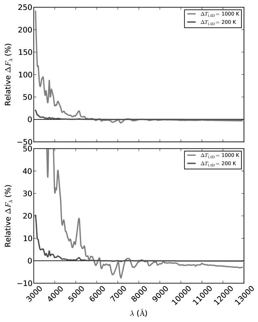
Figure 3: Relative difference between two FF 1:1 1.5D spectra, $\Delta T_{\mathrm{1.5D}}$ = 200 and 1000 K, and 1D spectra with equivalent $T_{\mathrm{eff,S-B}}$ = 4254 and 4336 K, respectively. The bottom panel shows an expanded y-scale view to reveal additional detail not visible on the larger scale of the top panel.

We attempted to recover the $T_{\mathrm{eff}}$ values of the 1.5D stars using three different methods of fitting 1D models: UBVRI photometry, spectrophotometry, and spectroscopy. Common to each method of post-processing, the 1.5D SEDs were interpolated from their initial wavelength distribution to a new distribution with a constant $\Delta\lambda$ of 0.006 Å. As a preliminary test to see which diagnostics would be expected to return $T_{\mathrm{eff}}$ values close to $T_{\mathrm{eff,S-B}}$, and which would return values differing from $T_{\mathrm{eff,S-B}}$, we examined the relative difference between two of our 1:1 FF spectra, $\Delta T_{\mathrm{1.5D}}$ = 200 and 1000 K, and 1D models with their equivalent $T_{\mathrm{eff,S-B}}$. These spectra were convolved with a Gaussian kernel of FWHM = 50 Å, representative of the nominal resolution element of the observed spectrophotometry in the Burnashev catalogue Burnashev (1985), prior to taking the differences. While there is little difference between the 1D and 1.5D in the near-IR and parts of the visible wavebands, they begin to diverge rapidly in the UV as seen in Fig. 3. This suggests that diagnostic tools focused on redder wavelengths are more likely to return $T_{\mathrm{eff}}$ values close to $T_{\mathrm{eff,S-B}}$. A more detailed high-resolutions analysis at the level of individual spectral lines could reveal specific diagnostics that are robust against 2D effects, but was beyond the scope of this study.

2.2.1 UBVRI photometry

For each of the NLTE and LTE 1D and NLTE 1.5D SEDs, photometric colors were produced using Bessel’s updated Johnson-Cousins UBVRI photometry (Bessell, 1990). The transmission data for each filter were interpolated to the wavelength distribution using quadratic splines. Five different color indices, U_x-B_x, B-V, V-R, V-I, and R-I, were calculated to milli-magnitude precision for each of the SEDs. It should be noted that the U band is of limited accuracy as the short wavelength cutoff in the observational U band is not defined by the instrumental configuration, but rather ozone absorption in Earth’s atmosphere. Because ozone column density varies by $\sim$20 % with geographic location and season, it is difficult to accurately reproduce U band photometry synthetically from models. These values were calibrated with a PHOENIX NLTE synthesized SED for the standard star Vega ($\alpha$ Lyr, HR7001, HD172167), using a single-point photometric calibration independent of color.

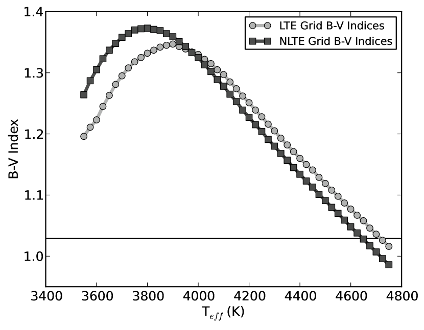
Figure 4: B-V color index values for the LTE and NLTE 1D SEDs. The turnover occurs at $T_{\mathrm{eff}}$ = 3900 K for the LTE SEDs and at $T_{\mathrm{eff}}$ = 3800 K for the NLTE SEDs. The solid black line indicates the value of the B-V index for the $\Delta T_{\mathrm{1.5D}}$ = 1000 K, 1:1 FF 1.5D SED.

While three of the five color indices for the 1D SEDs behaved as expected from the behavior of $B{}_{\lambda}$, with their values monotonically increasing for decreasing $T_{\mathrm{eff}}$ values over the range of the 1D SEDs, both the U_x-B_x and B-V indices stopped increasing and started decreasing at $T_{\mathrm{eff}}$ = 3900 K for the LTE SEDs, and at $T_{\mathrm{eff}}$ = 3800 K for the NLTE SEDs. This turnover is observed in stars, but between $T_{\mathrm{eff}}$ = 3540 K and 3380 K for the U-B index (Cox, 2000). The phenomenon is caused by spectral features in the B filter growing in strength more rapidly with decreasing $T_{\mathrm{eff}}$ values than those in the U filter, and reverses the trend in the color index expected from $B{}_{\lambda}$. Likewise, the spectral features in the V filter grow more rapidly than those in the B filter. In this case, the incorrect prediction of the $T_{\mathrm{eff}}$ value of the turnover is caused by the excess blue and UV flux common to PHOENIX models of cool red giant stars (Short & Hauschildt, 2003). Fig. 4 shows the B-V index value trend, including turnover, for both the LTE and NLTE 1D SEDs.

To quantify the errors from fitting 1D NLTE and LTE photometry to NLTE 2D stars, the library of 1D color index values was fitted to each of the 1.5D color index values. The closest matching $T_{\mathrm{eff}}$ value was found by means of inspection. Whichever 1D SED had the smallest difference between its value and the 1.5D value for each index was chosen as the match. For example, Fig. 4 shows the value of the B-V index for the 1.5D SED of 1:1 FF with $\Delta T_{\mathrm{1.5D}}$ = 1000 K including the region of closest match to 1D B-V values. Because of the degeneracy caused by the turnover in the U_x-B_x and B-V indices and the limiting $T_{\mathrm{eff}}$ numerical resolution of the 1D grid, it was possible that the best matching $T_{\mathrm{eff}}$ value would fall outside of the range of temperatures enclosed by the cool and hot 1D components, and would not be the correct match. Automatically limiting the best match to within the components’ $T_{\mathrm{eff}}$ range was determined to be too restrictive, so the closest three matches for both of the indices were found and ranked in order, whereupon the correct best match was chosen by inspection to logically fit the $T_{\mathrm{eff}}$ range.

2.2.2 SEDs and Spectra

Spectrophotometry

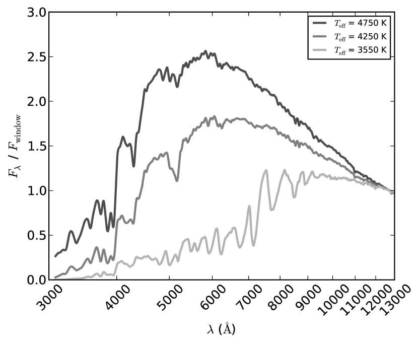
Figure 5: Relative version of three NLTE SEDs with $T_{\mathrm{eff}}$ values of 4750 K, 4250 K, and 3550 K.

Absolute surface flux SEDs, $F_{\lambda}$, of the 1.5D models were fitted with 1D SEDs to find the closest match to the the total energy radiated by the 1.5D stars; the relative flux SEDs were fitted with 1D relative SEDs to find the closest match to the overall shape of the 1.5D SEDs. For the relative flux SEDs, the surface flux values were normalized to the average flux within a 10 Å window ($F_{\mathrm{window}}$) located between $\lambda$ = 12750 and 12760 Å in the Rayleigh-Jeans tail of each SED. A 10 Å window was chosen over a single data point to avoid having selected a point that unreliably represents the continuum level in different SEDs. This window was chosen over others in the Rayleigh-Jeans tail because, it regularly had the fewest and weakest spectral features contained within its bounds. Fig. 5 displays the relative version of the NLTE SEDs with $T_{\mathrm{eff}}$ values of 4750 K, 4250 K, and 3550 K.

Spectroscopy

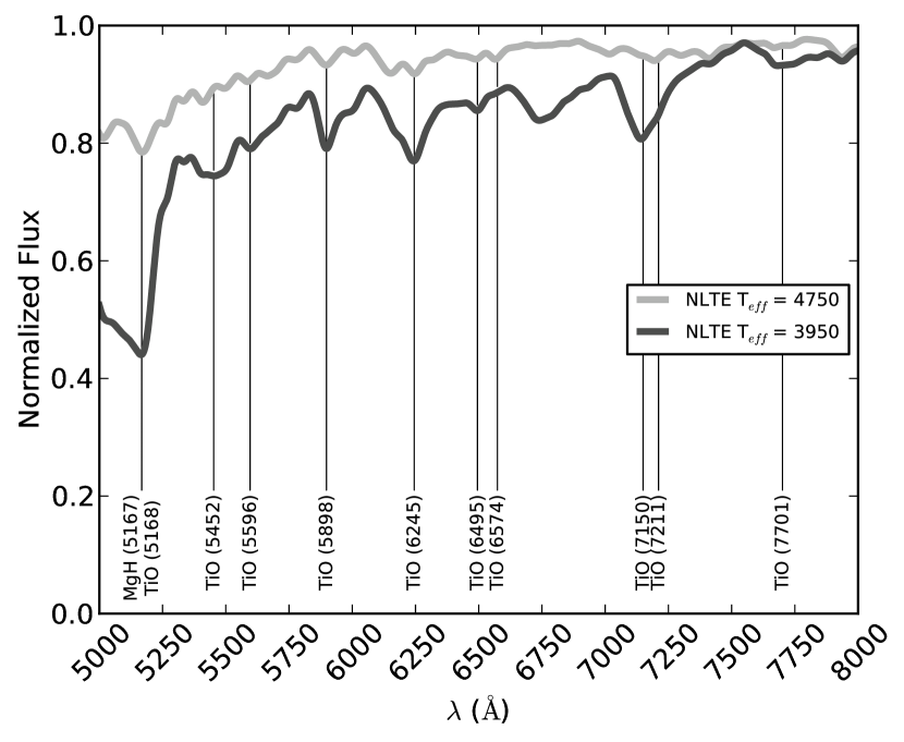
Figure 6: Flattened NLTE 1D spectra with $T_{\mathrm{eff}}$ = 4750 K and 3950 K, restricted to a wavelength range of $\lambda$ = 5000 to 8000 Å. Strong molecular absorption features in the region have been identified to illustrate the difference in temperature dependence of the MgH and TiO features.

Continuum normalized spectra were fitted with 1D spectra to determine the closest match based upon the relative strength of the spectral features. Continuum normalization was done for the 1D spectra by dividing the blanketed spectra by the corresponding continuum spectra. For the 1.5D SEDs, the same continuum normalization process was used, where the 1.5D synthetic continua were generated the same way that the 1.5D SEDs were, by linearly averaging the two corresponding 1D synthetic continua together. Initial fitting of the full wavelength range showed that the 1.5D spectra could be fit well by 1D spectra in the blue/UV and the near IR wavebands, but showed a large discrepancy over most of the optical waveband between $\lambda$ = 4800 and 8000 Å. This discrepancy, caused primarily by the distinctive TiO molecular absorption bands present in cool star spectra (Davies et al., 2013), prompted a second fitting diagnostic for the continuum normalized spectra, by restricting the fit to the wavelength range between $\lambda$ = 5500 and 8000 Å. An MgH band centered at 5167 Å was found to overlap with the TiO band near this wavelength range, and depended differently on $T_{\mathrm{eff}}$ than the TiO bands, affecting the quality of the fits. The overlapping MgH and TiO bands and additional nearby TiO bands are displayed in Fig. 6, illustrating the different temperature dependence of the features.

Each of the high resolution 1D and 1.5D SEDs were convolved with a Gaussian kernel of FWHM = 50 Å. The smoothed SEDs were then re-sampled to a much coarser $\Delta\lambda$ spacing to more accurately reflect the number of degrees of freedom available when comparing with an observed SED, but still fine enough to critically sample every feature remaining after the smoothing convolution. This amounted to a sample of 4000 wavelength points spaced between $\lambda$ = 3100 and 12900 Å, with 100 Å at each end of the original wavelength range having been lost to convolution edge effects. For both $F_{\lambda}$ and relative surface fluxes, the new points were evenly distributed in logarithmic space instead of linear space, amounting to taking the log of the upper and lower bounds of the wavelength region, distributing the new sample points evenly between these values, and then exponentiating everything to return to linear space. This resulted in a distribution of wavelength points with smaller $\Delta\lambda$ at shorter wavelengths and larger $\Delta\lambda$ at longer wavelengths. The motivation behind this was to attribute additional weight to spectral features located in the blue end of the SED when determining a best fit, without arbitrarily weighting select wavelength regions more heavily or determining a best fit for these regions separate from the rest of the SED altogether. Extra weighting was attributed to the blue band of the wavelength range because there are more spectral features per $\Delta\lambda$ interval there, and it is more sensitive to changes in temperature than the red band, making it a more sensitive diagnostic tool for determining $T_{\mathrm{eff}}$. The continuum normalized spectra were re-sampled in linear wavelength space to not grant any of the spectral features additional weight in the final fitting process. Unlike the spectrophotometric SEDs, the relative strengths of individual spectral features are of interest here, not the overall shape of the spectrum.

In all cases, the best fit 1D spectrum was determined by minimizing a modified Pearson $\chi^{2}$ test statistic, of the form

$$\chi^{2}=\frac{1}{n}\sum_{i=1}^{n}\frac{\left(1-M_{i}/O_{i}\right)^{2}}{M_{i}/O_{i}}.$$ (2)

where $n$ is the number of degrees of freedom, $O_{i}$ is the observed frequency of a phenomenon to be fitted, and $M_{i}$ is the modeled or expected frequency of the phenomenon. The 1D and 1.5D fluxes were treated as the modeled and observed frequencies, respectively, because a spectral flux is in some sense the frequency at which photons of given energies emerge from stars. For each 1.5D SED, every 1D SED was individually treated as the model value to create a test statistic value. The 1D SED with the minimum $\chi^{2}$ value was chosen as the best fitting SED from which the 1.5D $T_{\mathrm{eff}}$ value was inferred. In each fitting case, the result was determined to be significant at a confidence level of $p$ = 0.05. As a check for self consistency, the 1D NLTE fitted results are expected to be bounded by the hot and cold components’ $T_{\mathrm{eff}}$ values for a given 1.5D star, but this restriction is not expected of the 1D LTE fitted results.

3 RESULTS OF 1D $T_{\mathrm{eff}}$ FITTING

For all cases except one, the best fitting $T_{\mathrm{eff}}$ values for the 1.5D stars showed an increasing trend with increasing $\Delta T_{\mathrm{1.5D}}$. This is expected from the non-linear dependence of $B_{\lambda}$ on temperature, where a hotter $T_{\mathrm{eff}}$ value produces disproportionately more flux than a cooler one, and the averaged flux in 1.5D stars will be more than a $T_{\mathrm{eff}}$ value of 4250 K would suggest for a 1D star. This effect is even more pronounced at bluer wavelengths. Taking the derivative of $B_{\lambda}$ with respect to temperature,

$$\frac{\partial B_{\lambda}}{\partial T}=\frac{2h^{2}c^{3}}{\lambda^{6}k_{B}T_{\mathrm{eff}}^{2}}\frac{e^{hc/\lambda k_{B}T}}{\left(e^{hc/\lambda k_{B}T}-1\right)^{2}},$$ (3)

inspection reveals that for changing temperatures, $B_{\lambda}$ exhibits larger relative changes at shorter wavelengths, causing the flux at the blue end of the spectrum to increase disproportionately faster than the rest of the wavelength range with increasing $T_{\mathrm{eff}}$.

For the case of the TiO bands fitted in the continuum normalized spectra, the reverse trend was instead seen; a decreasing best fit $T_{\mathrm{eff}}$ value with increasing $\Delta T_{\mathrm{1.5D}}$. This is expected from the non-linear dependence of molecule formation on gas temperature (Uitenbroek & Criscuoli, 2011). All fitting results are considered as having a formal uncertainty of $\delta T=\pm$25 K, one half of the original numerical temperature resolution of the 1D grid. The fit results are summarized in Tables 4 and 5, while Tables 6 and 7 display the differences between the fit results and the 1.5D $T_{\mathrm{eff,S-B}}$. Results for comparing with 1D LTE spectra are limited to diagnostics only involving V-band photometry and redder, or equivalent wavelength ranges, as discussed in section 2.1.

3.1 UBVRI photometry

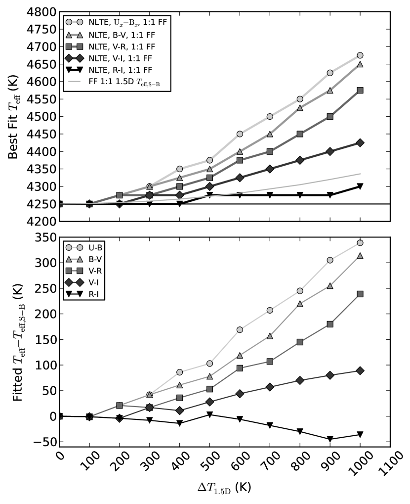
Figure 7: Inferred $T_{\mathrm{eff}}$ values as functions of the difference in 1.5D component $T_{\mathrm{eff}}$, $\Delta T_{\mathrm{1.5D}}$, for five photometric color indices and 1:1 FF. The top image displays the fit values and the 1.5D $T_{\mathrm{eff,S-B}}$, with the solid black line representing $T_{\mathrm{eff,R-J}}$ = 4250 K, and the bottom displays these difference between these values and $T_{\mathrm{eff,S-B}}$ for a given $\Delta T_{\mathrm{1.5D}}$.

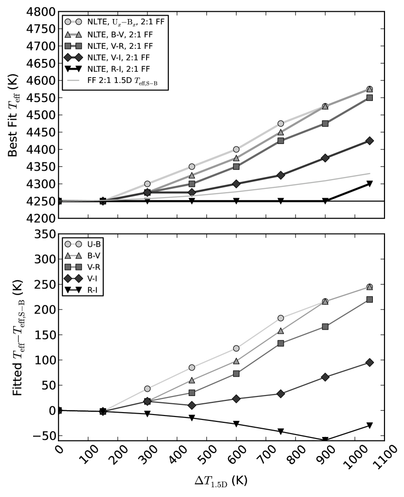
Figure 8: Same as Fig. 7, but for 2:1 FF.

Figs. 7 and 8 presents each of the five photometric color indices’ NLTE best fitting $T_{\mathrm{eff}}$ values as functions of $\Delta T_{\mathrm{1.5D}}$ for all of the 1.5D stars. Each of the color indices shows increasing best fit $T_{\mathrm{eff}}$ values for the 1.5D stars with increasing $\Delta T_{\mathrm{1.5D}}$. The slope of the $T_{\mathrm{eff}}\left(\Delta T_{\mathrm{1.5D}}\right)$ relation is different for the five indices, creating, for a given 1.5D star, a spread of best fit $T_{\mathrm{eff}}$ values among the indices that grows with increasing $\Delta T_{\mathrm{1.5D}}$. The slopes of the individual color indices’ fits are steeper for the bluer indices, and nearly flat for the R-I index over the $\Delta T_{\mathrm{1.5D}}$ range. Such a spread in the fits shows that horizontal inhomogeneity effects are non-constant across the spectrum. This spread cannot be resolved at a 25 K resolution for $\Delta T_{\mathrm{1.5D}}\leq$ 150 K, and grows as large as 375 K for 1.5D stars with 1:1 FF, and as large as 250 K for 2:1 FF.

For the 2:1 FF fits, the spread is not as large as the 1:1 FF, because, while the 2:1 1.5D star is created with more hot material than cool material, the $T_{\mathrm{eff}}$ values of both components are lower than the respective components of a 1:1 1.5D star having the same $\Delta T_{\mathrm{1.5D}}$, outweighing the contribution of more hot material by having less flux to contribute from the hot component. This resulted in either the same or lower temperature fits for a given $\Delta T_{\mathrm{1.5D}}$. Additionally, because the cool component of the 2:1 1.5D stars has a lower $T_{\mathrm{eff}}$ value than that of a 1:1 1.5D star, the blue and UV regions are even more severely line-blanketed, contributing even less flux than the difference in 1D $T_{\mathrm{eff}}$ values alone would suggest, and resulting in lower temperature fits for the color indices at shorter wavelengths, noticeably U_x-B_x and B-V.

NLTE

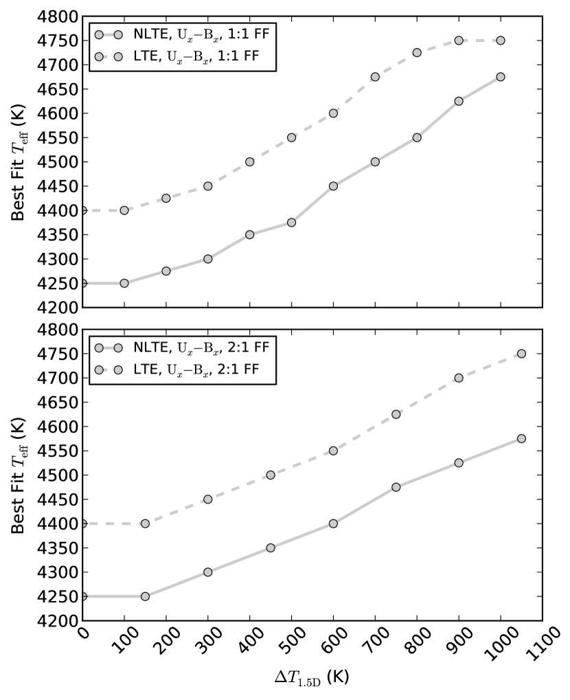
Figure 9: U_x-B_x index best fit $T_{\mathrm{eff}}$ value results. The top image contains results for 1.5D stars with 1:1 FF, while the bottom image contains those for 2:1 FF. Results from NLTE (solid lines) and LTE (dashed lines) 1D modeling. The data points for the LTE 1:1 FF fits at $\Delta T_{\mathrm{1.5D}}$ = 900K and 1000 K are at the upper limit of the 1D grid of models and may not accurately represent what the best fitting $T_{\mathrm{eff}}$ values may be.

To quantify the magnitude of NLTE effects, we defined the quantity $\Delta T_{\mathrm{NLTE}}$ as the difference between the fitted NLTE $T_{\mathrm{eff}}$ value and the fitted LTE $T_{\mathrm{eff}}$ value for a 1.5D star. Examining each color index individually for the effects of NLTE, it is seen that both choices of FF return LTE best fit $T_{\mathrm{eff}}$ values that are always hotter than the NLTE best fits for a given $\Delta T_{\mathrm{1.5D}}$, and that $\Delta T_{\mathrm{NLTE}}$ is approximately constant within one numerical temperature resolution unit for all choices of $\Delta T_{\mathrm{1.5D}}$ for each color index. This constant value depends on color index, suggesting that NLTE effects are non-constant across the spectrum, but they are temperature independent over the range of $T_{\mathrm{eff}}$ values in the 1D grid. For the U_x-B_x index, the magnitude of $\Delta T_{\mathrm{NLTE}}$ is at least 100 K larger than the other indices because of the greater flux in the blue and UV from NLTE Fe I overionization, forcing the LTE SEDs to have a higher $T_{\mathrm{eff}}$ value to match the flux. Fig. 9 displays the results for the U_x-B_x index, showing a nearly constant value for $\Delta T_{\mathrm{NLTE}}$ of -150 K to -175 K. The plateau in the LTE 1:1 FF $T_{\mathrm{eff}}\left(\Delta T_{\mathrm{1.5D}}\right)$ relation above $\Delta T_{\mathrm{1.5D}}$ = 800 K is not a breaking of this constant $\Delta T_{\mathrm{NLTE}}$, but rather the best fit $T_{\mathrm{eff}}$ values were restricted by the upper limit of the 1D grid of models.

3.2 Spectrophotometry

3.2.1 Absolute flux distributions

Both choices of FF show an increasing trend in NLTE best fitting $T_{\mathrm{eff}}$ values for increasing $\Delta T_{\mathrm{1.5D}}$. For values of $\Delta T_{\mathrm{1.5D}}\leq$ 300 K, both choices of FF produce the same best fitting $T_{\mathrm{eff}}$ value for a given $\Delta T_{\mathrm{1.5D}}$ value, whereas for values of $\Delta T_{\mathrm{1.5D}}\geq$ 400 K, the 1:1 FF 1.5D SEDs produce hotter $T_{\mathrm{eff}}$ values than the 2:1 FF SEDs. The 1:1 FF SEDs reached a best fitting $T_{\mathrm{eff}}$ value of 4450 K and the 2:1 FF SEDs reached 4425 K at maximum $\Delta T_{\mathrm{1.5D}}$.

NLTE

Comparing the LTE results with the NLTE results for both choices of FF, and for every value of $\Delta T_{\mathrm{1.5D}}$, the LTE best fitting $T_{\mathrm{eff}}$ values are hotter than the NLTE values. Because NLTE stars produce more blue and UV flux for a given $T_{\mathrm{eff}}$ value than LTE stars, the LTE 1D SEDs returned higher best fitting $T_{\mathrm{eff}}$ values to match the $F_{\lambda}$ value of the 1.5D SED. For the 1:1 FF 1.5D SEDs, $\Delta T_{\mathrm{NLTE}}$ varied between 25 K and 50 K, whereas for the 2:1 FF SEDs, $\Delta T_{\mathrm{NLTE}}$ was nearly constant at 50 K, only dropping to 25 K for $\Delta T_{\mathrm{1.5D}}$ = 900 K.

3.2.2 Relative flux distributions

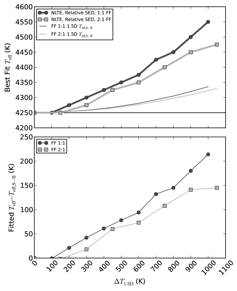
Figure 10: Inferred $T_{\mathrm{eff}}$ from fitting relative surface flux SEDs with 1D NLTE SEDs. The top image displays the fit values and the 1.5D $T_{\mathrm{eff,S-B}}$, with the solid black line representing $T_{\mathrm{eff,R-J}}$ = 4250 K, and the bottom displays these difference between these values and $T_{\mathrm{eff,S-B}}$ for a given $\Delta T_{\mathrm{1.5D}}$.

The results of fitting 1D NLTE relative flux SEDs to the 1.5D SEDs are presented in Fig. 10. Both choices of FF show an increasing trend in best fitting $T_{\mathrm{eff}}$ values for increasing $\Delta T_{\mathrm{1.5D}}$ with the 1:1 FF best fitting $T_{\mathrm{eff}}$ values being hotter than the 2:1 best fits at every value of $\Delta T_{\mathrm{1.5D}}>$ 100 K. The 1:1 FF SEDs reached a best fitting $T_{\mathrm{eff}}$ value of 4550 K and the 2:1 FF SEDs reached 4475 K at maximum $\Delta T_{\mathrm{1.5D}}$. Because the logarithmically spaced $\lambda$ grid was utilized to place more weight on bluer wavelengths for the fits, the 1.5D SED matches well with the best fitting 1D SED for $\lambda\lesssim$ 4500 Å, but the 1D SED fails to predict the shape of the 1.5D SED around the peak of the spectrum; here, the 1.5D SED would be fit by a SED with less flux at these wavelengths relative to $F_{\mathrm{window}}$, suggesting a cooler $T_{\mathrm{eff}}$ value for the best fitting 1D SED.

NLTE

The LTE best fitting $T_{\mathrm{eff}}$ values are hotter than the NLTE values for every value of $\Delta T_{\mathrm{1.5D}}$. For both choices of FF, $\Delta T_{\mathrm{NLTE}}$ varied between 50 K and 75K.

3.3 Spectroscopy

3.3.1 Continuum normalized spectra

The best fit $T_{\mathrm{eff}}$ values below $\Delta T_{\mathrm{1.5D}}$ = 500 K are approximately equal at each $\Delta T_{\mathrm{1.5D}}$ for both choices of FF, and only begin to differ above $\Delta T_{\mathrm{1.5D}}$ = 600 K, with the 1:1 FF 1.5D stars having hotter fitted values. The inequality reaches a maximum $T_{\mathrm{eff}}$ value difference of 100 K at the maximum $\Delta T_{\mathrm{1.5D}}$, with the 1:1 FF 1.5D stars reaching a maximum $T_{\mathrm{eff}}$ value of 4650 K.

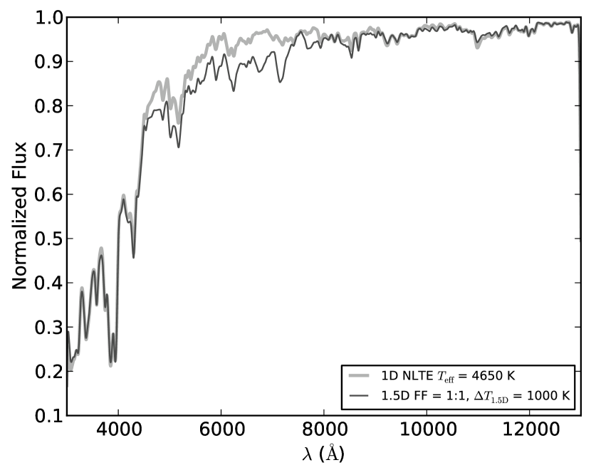
Figure 11: Continuum normalized 1.5D 1:1 FF with the best fitting 1D NLTE spectrum. The drop off below $\sim$ 6000 Å is caused by the extreme level of line blanketing in the blue and UV. The poor fit between $\sim$ 4500 and 8000 Å is attributed to prominent TiO absorption features present in the cool component of the 1.5D spectrum.

Fig. 11 shows the 1.5D 1:1 FF continuum normalized spectrum with $\Delta T_{\mathrm{1.5D}}$ = 1000 K plotted with the best fitting 1D NLTE spectrum and two bracketing 1D NLTE spectra. The best fitting 1D spectrum is seen to be a good fit to the 1.5D spectrum for the blue and red ends of the $\lambda$ range, but is a poor match between $\lambda\approx$ 4500 and 8000 Å. In this region, the 1.5D spectrum exhibits stronger spectral features than the best fitting 1D spectrum would imply, suggesting that there is a cooler best fitting $T_{\mathrm{eff}}$ value for this region. Additional fits omitting the poorly matched region were performed and the resultant $T_{\mathrm{eff}}$ values were found to differ by less than one numerical temperature resolution unit from the fits performed over the entire range, at maximum $\Delta T_{\mathrm{1.5D}}$.

NLTE

Comparing the NLTE results with LTE results, it is seen that for both FF values, the LTE best fit $T_{\mathrm{eff}}$ values are hotter than the NLTE fits, but $\Delta T_{\mathrm{NLTE}}$ increases with increasing $\Delta T_{\mathrm{1.5D}}$. For the 2:1 FF 1.5D stars, $\Delta T_{\mathrm{NLTE}}$ reaches a maximum of 175 K, and for the 1:1 FF stars, it is potentially even larger but the LTE results plateau above $\Delta T_{\mathrm{1.5D}}$ = 800 K, similar to the U_x-B_x photometric color index in Section 3.1, and for the same reasons.

3.3.2 TiO bands

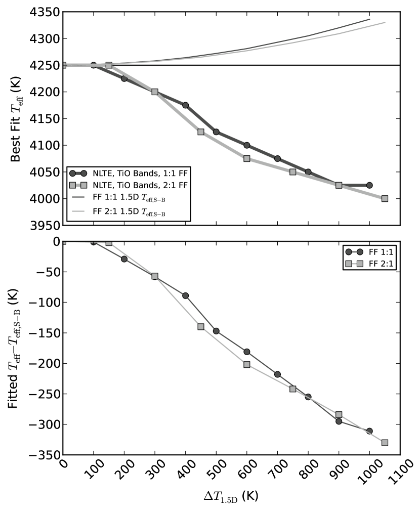
Figure 12: Same as Fig. 10 but for TiO bands in continuum normalized spectra.

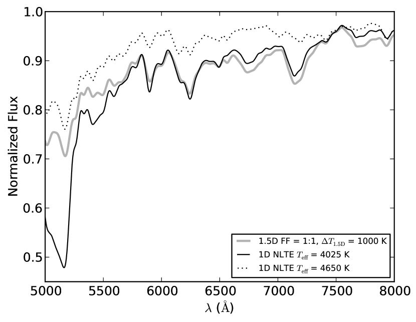
Figure 13: Continuum normalized 1.5D 1:1 FF with the best fitting 1D NLTE spectrum (solid black) for the TiO band $\lambda$ range from 5500 to 8000 Å. The best fitting 1D NLTE spectrum (dotted) from fitting the full $\lambda$ range is also shown to obviate the necessity of fitting this region independently.

Fig. 12 shows NLTE best fitting $T_{\mathrm{eff}}$ values inferred from fitting to continuum normalized spectra restricted to the TiO bands located between $\lambda$ = 5500 and 8000 Å for all 1.5D stars. A decreasing trend of fitted $T_{\mathrm{eff}}$ value with increasing $\Delta T_{\mathrm{1.5D}}$ is observed, dropping as low as $T_{\mathrm{eff}}$ = 4000 K at maximum $\Delta T_{\mathrm{1.5D}}$. This agrees with the observation from section 3.3.1 that the best fitting $T_{\mathrm{eff}}$ values for this $\lambda$ should be cooler than those found for the same star when fitting the entire visible band. Fig 13 shows the TiO fitting region of the 1.5D 1:1 $\Delta T_{\mathrm{1.5D}}$ = 1000 K with the best fitting 1D spectrum found for this region, as well as the 1D spectrum found for fitting the entire $\lambda$ range as a comparison. Both of the FF values produce similar results when fit with NLTE 1D stars, the fits being separated by no more than one numerical temperature resolution unit at any $\Delta T_{\mathrm{1.5D}}$. The 1:1 FF 1.5D stars have the hotter fitted $T_{\mathrm{eff}}$ values at $\Delta T_{\mathrm{1.5D}}$ values greater than 600 K. The TiO molecular bands grow in strength so rapidly with decreasing $T_{\mathrm{eff}}$ that the hot component does not dominate the fit in the TiO band region as it does for the overall continuum normalized spectra. The cool component now dominates the shape, with the hot component only mitigating the effect, pulling the fits to lower temperatures with increasing $\Delta T_{\mathrm{1.5D}}$.

NLTE

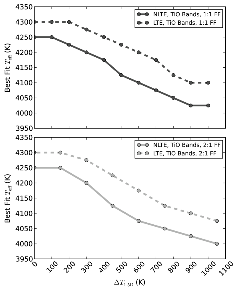
Figure 14: Same as Fig. 9 but for best fitted $T_{\mathrm{eff}}$ from fitting TiO bands.

The LTE results are hotter than the respective NLTE results at each $\Delta T_{\mathrm{1.5D}}$ for both choices of FF, as seen in Fig. 14. This is not caused directly by an NLTE effect, such as Fe I overionization as in the previous four methods, as PHOENIX does not compute molecules in NLTE. Instead it is an indirect effect of the difference of LTE and NLTE $T_{\mathrm{Kin}}\left(\tau\right)$ structures in the upper atmosphere, and only 1.5D modeling of this style has revealed its role. For a given $T_{\mathrm{eff}}$, NLTE models are generally hotter than LTE models in the upper atmosphere above $\tau_{12000}$ = 1, as seen in Fig. 2. Because of this, more TiO molecules will collisionally dissociate in the upper atmosphere of a NLTE star than an LTE star, and NLTE stars will form weaker absorption features. Therefore, NLTE best fits will be required to have lower $T_{\mathrm{eff}}$ values to match the strength of the TiO absorption features. In this case $\Delta T_{\mathrm{NLTE}}$ is non constant as a function of $\Delta T_{\mathrm{1.5D}}$, increasing from 50 K at $\Delta T_{\mathrm{1.5D}}$ = 0 K, to a local maximum of 100 K, then decreasing back to 75 K at maximum $\Delta T_{\mathrm{1.5D}}$, for both FF.

4 SUMMARY AND CONCLUSIONS

The goal of this work has been to analyze the effects of massively NLTE atmospheric modeling combined with 2D horizontal inhomogeneities on $T_{\mathrm{eff}}$ values inferred from SEDs and line profiles. The stellar atmosphere and spectrum synthesis code PHOENIX was used to generate a grid of spherical stellar atmosphere models in both LTE and NLTE, and to synthesize spectra for the models.

Spectra of target 2D “observed” stars were produced in the 1.5D approximation by linearly averaging two NLTE 1D spectra together under two different weighting schemes (FF), such that the $T_{\mathrm{eff,R-J}}$ was 4250 K and the temperature difference between the 1D was as large as $\Delta T_{\mathrm{1.5D}}$ = 1050 K. The grid of LTE and NLTE 1D SEDs and spectra were fit to the observations to infer $T_{\mathrm{eff}}$ values for the 1.5D stars using five different approaches. All inferred $T_{\mathrm{eff}}$ values and differences between inferred $T_{\mathrm{eff}}$ and 1.5D $T_{\mathrm{eff,S-B}}$ are considered to have a formal uncertainty of 25 K, half of one temperature resolution unit in our pre-interpolated 1D grid.

Photometric colors of 1D stars computed from synthetic UBVRI photometry were compared to 1.5D colors to assess the errors in photometrically derived $T_{\mathrm{eff}}$ values. For the five color indices and both values of FF, the inferred value of $T_{\mathrm{eff}}$ was seen to increase with $\Delta T_{\mathrm{1.5D}}$, and increased at a greater rate for indices that involved bluer wavebands. When the LTE and NLTE results were compared, the $T_{\mathrm{eff}}$ values inferred from fitting LTE colors were systematically higher than their NLTE counterparts. The magnitude of $\Delta T_{\mathrm{NLTE}}$ was approximately constant as a function of $\Delta T_{\mathrm{1.5D}}$ in all cases. The value was largest when comparing U_x-B_x inferred $T_{\mathrm{eff}}$ values, and decreased for redder indices.

Absolute surface flux 1D SEDs were fit to the 1.5D SEDs to assess how changes to the predicted bolometric flux introduced by the modeling assumptions affect the inferred value of $T_{\mathrm{eff}}$. For both values of FF, the inferred value of $T_{\mathrm{eff}}$ was seen to increase with $\Delta T_{\mathrm{1.5D}}$. This approach showed the lowest overall error of any of the full $\lambda$ distribution fitting approaches in the inferred value of $T_{\mathrm{eff}}$; only 110 K difference between the fit $T_{\mathrm{eff}}$ value and $T_{\mathrm{eff,S-B}}$ at maximum $\Delta T_{\mathrm{1.5D}}$. Again, the inferred $T_{\mathrm{eff}}$ values from fitting LTE SEDs were systematically higher than those from fitting NLTE SEDs, and the magnitude of $\Delta T_{\mathrm{NLTE}}$ was approximately constant as a function of $\Delta T_{\mathrm{1.5D}}$.

Relative 1D SEDs normalized to the average continuum flux in a 10 Å window in the R-J tail were fit to the 1.5D SEDs to assess how the modeling assumptions affect overall shape of the SED and the temperature sensitive spectral features located in the blue and near-UV bands. For both values of FF, the inferred value of $T_{\mathrm{eff}}$ was seen to increase with $\Delta T_{\mathrm{1.5D}}$. The inferred $T_{\mathrm{eff}}$ values from fitting LTE SEDs were systematically higher than those from fitting NLTE SEDs, and the magnitude of $\Delta T_{\mathrm{NLTE}}$ was approximately constant as a function of $\Delta T_{\mathrm{1.5D}}$. These three complimentary methods (photometric colors, absolute surface flux SEDs, and relative SEDs) show results consistent with each other.

Of the three spectrophotometric methods, the photometric colors give both the highest and the lowest errors on the estimates of the $T_{\mathrm{eff}}$. At maximum $\Delta T_{\mathrm{1.5D}}$, the U_x-B_x index fitting returned up to 340 K higher than $T_{\mathrm{eff,S-B}}$, while the R-I index returned as low as 60 K less than $T_{\mathrm{eff,S-B}}$. The V-I fitting resulted in error values similar to that of the absolute SEDs, with fitted $T_{\mathrm{eff}}$ values as high as 90 K above $T_{\mathrm{eff,S-B}}$. The relative SED fitting returned error values similar to the V-R index, as high as 210 and 240 K above $T_{\mathrm{eff,S-B}}$ respectively. Together, these results reinforce that red/near-IR photometry is more reliable for diagnosing $T_{\mathrm{eff}}$ in stars with significant horizontal inhomogeneity.

Continuum normalized 1D spectra spanning a wavelength distribution between $\lambda$ = 3000 and 13000 Å were fit to the 1.5D spectra to assess how the modeling assumptions change the predicted strength of spectral features. For both values of FF, the inferred value of $T_{\mathrm{eff}}$ was seen to increase with $\Delta T_{\mathrm{1.5D}}$. It is important to note that this result is consistent with the spectrophotometric results, even though it is arrived at through a complimentary method. This approach showed the highest overall error of any of the full spectrum fitting approaches in the inferred value of $T_{\mathrm{eff}}$; 310 K above $T_{\mathrm{eff,S-B}}$ at maximum $\Delta T_{\mathrm{1.5D}}$. The inferred $T_{\mathrm{eff}}$ values from fitting LTE spectra were systematically higher than those from fitting NLTE spectra, and the magnitude of $\Delta T_{\mathrm{NLTE}}$ was approximately constant as a function of $\Delta T_{\mathrm{1.5D}}$.

Predicted line profiles for the important 1D TiO bands spanning a wavelength range between $\lambda$ = 5500 and 8000 Å were fit to the 1.5D TiO bands to assess how the strength of molecular features found primarily in the cold component of the 1.5D stars affect the inferred value of $T_{\mathrm{eff}}$. This was the only approach to show the inferred value of $T_{\mathrm{eff}}$ decreasing with increasing $\Delta T_{\mathrm{1.5D}}$. The rapid nonlinear growth of molecular features with decreasing temperature became the dominant aspect in determining the $T_{\mathrm{eff}}$ value, over the nonlinear contribution to the average flux from the higher temperature 1.5D component. The inferred $T_{\mathrm{eff}}$ values from fitting LTE spectra were still systematically higher than those from fitting NLTE spectra, and the magnitude of $\Delta T_{\mathrm{NLTE}}$ was approximately constant as a function of $\Delta T_{\mathrm{1.5D}}$.

In this work we have shown that the approximations of both horizontal homogeneity and LTE introduce errors in the value of $T_{\mathrm{eff}}$ inferred from fitting quantities derived from models to observed quantities. By assuming both horizontal homogeneity and LTE, the inferred $T_{\mathrm{eff}}$ values may differ from the $T_{\mathrm{eff,S-B}}$ of a star by 340 K or more, depending on the quantity used to infer the $T_{\mathrm{eff}}$. Of the two values of FF, 1:1 produced hotter values of inferred $T_{\mathrm{eff}}$ in general. In simulating horizontal inhomogeneities it was seen that the bolometric flux of a 1.5D star increased with $\Delta T_{\mathrm{1.5D}}$, and a percentage of the flux was redistributed at bluer wavelengths. Spectral features in general appeared to have been produced by a star hotter than the $T_{\mathrm{eff,R-J}}$, except that strong molecular features found in cooler stars were also present in the spectra. Furthermore, for all five approaches, $\Delta T_{\mathrm{NLTE}}$ is approximately independent of $\Delta T_{\mathrm{1.5D}}$, and we conclude that the magnitude of the effect of NLTE on $T_{\mathrm{eff}}$ derived from fitting 1D models is approximately independent of the thermal contrast characterizing the degree of the horizontal inhomogeneity of the star being modeled, and only dependent on the observable quantity being fit.

While $\Delta T_{\mathrm{1.5D}}$ was the only parameter varied in the scope of this study, other modeling parameters such as log $g$ and [Fe/H] are expected to have an impact on $T_{\mathrm{eff}}$ – $T_{\mathrm{eff,S-B}}$ and $T_{\mathrm{eff}}$ – $T_{\mathrm{eff,R-J}}$ derived in various ways for horizontally inhomogeneous stars. Both Samadi et al. (2013) and Tremblay et al. (2013) have shown the RMS temperature variations to increase with decreasing log $g$, and Tremblay et al. (2013) has also shown them to increase with decreasing [Fe/H]. Likewise, the values of the fitted $T_{\mathrm{eff}}$ – $T_{\mathrm{eff,S-B}}$ at a given $\Delta T_{\mathrm{1.5D}}$ are expected to differ with the $T_{\mathrm{eff,R-J}}$ of the 1.5D stars. Investigating these parameters requires extensive additions to our 1D grid of models, as well as an updated Fe I atomic model, and will be explored in a future study.

Table 1: List of atomic species treated in NLTE energy level calculations. Number of energy levels and line transitions included for each ionization stage are given.

Element	I	II
H	80/3160	$\cdots$ string
He	19/37string	$\cdots$ string
Li	57/333string	55/124string
C	228/1387	$\cdots$ string
N	252/2313	$\cdots$ string
O	36/66string	$\cdots$ string
Ne	26/37string	$\cdots$ string
Na	53/142string	35/171string
Mg	273/835string	72/340string
Al	111/250string	188/1674string
Si	329/1871	93/436string
P	229/903string	89/760string
S	146/349string	84/444string
K	73/210string	22/66string
Ca	194/1029	87/455string
Ti	395/5279	204/2399string
Mn	316/3096	546/7767string
Fe	494/6903	617/13675
Co	316/4428	255/2725string
Ni	153/1690	429/7445string

Table 2: Wavelength grid spacing used in computing PHOENIX model atmospheres and spectra

Wavelength Range $\lambda$ (Å)	Spacing $\Delta\lambda$ (Å)	Mid Range Spectral Resolution $R$
3000 - string4000	0.010	350000
4000 - string5000	0.013	346000
5000 - string6000	0.016	344000
7000 - string8000	0.023	326000
8000 - 11000	0.027	352000
11000 - 13000string	0.037	324000

Table 3: 1.5D model components for 1:1 and 2:1 filling factors and resultant 1.5D $T_{\mathrm{eff,S-B}}$ (see Section 1.2) values. All 1.5D stars are considered to have $T_{\mathrm{eff,R-J}}$ = 4250 K.

	1:1 Filling Factor			2:1 Filling Factor
	Warm	Cool		Warm	Cool
	Component	Component	1.5D	Component	Component	1.5D
$\Delta T_{\mathrm{1.5D}}$ (K)	$T_{\mathrm{eff}}$ (K)	$T_{\mathrm{eff}}$ (K)	$T_{\mathrm{eff,S-B}}$ (K)	$T_{\mathrm{eff}}$ (K)	$T_{\mathrm{eff}}$ (K)	$T_{\mathrm{eff,S-B}}$ (K)
1050	$\cdots$	$\cdots$	$\cdots$	4600	3550	4330
1000	4750	3750	4336	$\cdots$	$\cdots$	$\cdots$
string900	4700	3800	4320	4550	3650	4309
string800	4650	3850	4305	$\cdots$	$\cdots$	$\cdots$
string750	$\cdots$	$\cdots$	$\cdots$	4500	3750	4292
string700	4600	3900	4293	$\cdots$	$\cdots$	$\cdots$
string600	4550	3950	4281	4450	3850	4277
string500	4500	4000	4272	$\cdots$	$\cdots$	$\cdots$
string450	$\cdots$	$\cdots$	$\cdots$	4400	3950	4265
string400	4450	4050	4264	$\cdots$	$\cdots$	$\cdots$
string300	4400	4100	4258	4350	4050	4257
string200	4350	4150	4254	$\cdots$	$\cdots$	$\cdots$
string150	$\cdots$	$\cdots$	$\cdots$	4300	4150	4252
string100	4300	4200	4251	$\cdots$	$\cdots$	$\cdots$
string0	4250	4250	4250	4250	4250	4250

Note. — The $T_{\mathrm{eff,S-B}}$ values are quoted to the closest K as computed.

Table 4: Best fit $T_{\mathrm{eff}}$ results for NLTE.

$\Delta T_{\mathrm{1.5D}}$	Ux-Bx	B-V	V-R	V-I	R-I	Absolute SED	Relative SED	Continuum Normalized Spectra	TiO Bands
$\mathbf{FF1:1}$
1000	4675	4650	4575	4425	4300	4450	4550	4650	4025
string900	4625	4575	4500	4400	4275	4425	4500	4575	4025
string800	4550	4525	4450	4375	4275	4400	4450	4525	4050
string700	4500	4450	4400	4350	4275	4375	4425	4475	4075
string600	4450	4400	4375	4325	4275	4350	4375	4425	4100
string500	4375	4350	4325	4300	4275	4325	4350	4375	4125
string400	4350	4325	4300	4275	4250	4300	4325	4350	4175
string300	4300	4300	4275	4275	4250	4275	4300	4300	4200
string200	4275	4275	4275	4250	4250	4275	4275	4275	4225
string100	4250	4250	4250	4250	4250	4250	4250	4250	4250
string0	4250	4250	4250	4250	4250	4250	4250	4250	4250
$\mathbf{FF2:1}$
1050	4575	4575	4550	4425	4300	4425	4475	4550	4000
string900	4525	4525	4475	4375	4250	4400	4450	4500	4025
string750	4475	4450	4425	4325	4250	4350	4400	4450	4050
string600	4400	4375	4350	4300	4250	4325	4350	4400	4075
string450	4350	4325	4300	4275	4250	4300	4325	4350	4125
string300	4300	4275	4275	4275	4250	4275	4275	4300	4200
string150	4250	4250	4250	4250	4250	4250	4250	4275	4250
string0	4250	4250	4250	4250	4250	4250	4250	4250	4250

Note. — All results are in K and have $\pm$ 25 K uncertainty.

Table 5: Same as Table 4 but for LTE. Only diagnostics that are insensitive to Fe I overionization in the blue/UV wavebands are displayed.

$\Delta T_{\mathrm{1.5D}}$	V-R	V-I	R-I	TiO Bands
$\mathbf{FF1:1}$
1000	4600	4475	4325	4100
string900	4525	4425	4325	4100
string800	4475	4400	4300	4125
string700	4425	4375	4300	4175
string600	4400	4350	4300	4200
string500	4350	4325	4300	4225
string400	4325	4300	4300	4250
string300	4300	4300	4300	4275
string200	4275	4300	4300	4300
string100	4275	4275	4300	4300
string0	4275	4275	4275	4300
$\mathbf{FF2:1}$
1050	4575	4450	4325	4075
string900	4500	4400	4300	4100
string750	4450	4375	4275	4125
string600	4375	4325	4275	4175
string450	4325	4300	4300	4225
string300	4300	4300	4300	4275
string150	4275	4275	4300	4300
string0	4275	4275	4275	4300

Note. — All results are in K and have $\pm$ 25 K uncertainty.

Table 6: Best fitting $T_{\mathrm{eff}}$ – 1.5D $T_{\mathrm{eff,S-B}}$ for NLTE.

$\Delta T_{\mathrm{1.5D}}$	Ux-Bx	B-V	V-R	V-I	R-I	Absolute SED	Relative SED	Continuum Normalized Spectra	TiO Bands
$\mathbf{FF1:1}$
1000	339	314	239	89	-36	114	214	314	-311
string900	305	255	180	80	-45	105	180	255	-295
string800	245	220	145	70	-30	95	145	220	-255
string700	207	157	107	57	-18	82	132	182	-218
string600	169	119	94	44	-6	69	94	144	-181
string500	103	78	53	28	3	53	78	103	-147
string400	86	61	36	11	-14	36	61	86	-89
string300	42	42	17	17	-8	17	42	42	-58
string200	21	21	21	-4	-4	21	21	21	-29
string100	-1	-1	-1	-1	-1	-1	-1	-1	-1
string0	0	0	0	0	0	0	0	0	0
$\mathbf{FF2:1}$
1050	245	245	220	95	-30	95	145	220	-330
string900	216	216	166	66	-59	91	141	191	-284
string750	183	158	133	33	-42	58	108	158	-242
string600	123	98	73	23	-27	48	73	123	-202
string450	85	60	35	10	-15	35	60	85	-140
string300	43	18	18	18	-7	18	18	43	-57
string150	-2	-2	-2	-2	-2	-2	-2	23	-2
string0	0	0	0	0	0	0	0	0	0

Note. — All results are in K. We choose to quote the values to the nearest K as computed, but they are understood to have $\pm$ 25 K uncertainty.

Table 7: Same as Table 6 but for LTE. Only diagnostics that are insensitive to Fe I overionization in the blue/UV wavebands are displayed.

$\Delta T_{\mathrm{1.5D}}$	V-R	V-I	R-I	TiO Bands
$\mathbf{FF1:1}$
1000	264	139	-11	-236
string900	205	105	5	-220
string800	170	95	-5	-180
string700	132	82	7	-118
string600	119	69	19	-81
string500	78	53	28	-47
string400	61	36	36	-14
string300	42	42	42	17
string200	21	46	46	46
string100	24	24	49	49
string0	25	25	25	50
$\mathbf{FF2:1}$
1050	245	120	-5	-255
string900	191	91	-9	-209
string750	158	83	-17	-167
string600	98	48	-2	-102
string450	60	35	35	-40
string300	43	43	43	18
string150	23	23	48	48
string0	25	25	25	50

Note. — All results are in K. We choose to quote the values to the nearest K as computed, but they are understood to have $\pm$ 25 K uncertainty.

References

- Alves-Brito et al. (2010) Alves-Brito, A., Melendez, J. Asplund, M., et al., 2010, A&A, 513, A35
- Asplund (2005) Asplund, M., 2005, ARA&A, 43, 481
- Asplund et al. (2009) Asplund, M., Grevesse, N., Sauval, A. J., et al., 2009, ARA&A, 47, 481
- Baron & Hauschildt (1998) Baron, E. & Hauschildt, P. H., 1998, ApJ, 495, 370
- Bergemann et al. (2013) Bergemann, M., Kudritzki, R. P., Davies, B., et al., 2013, EAS Publications Series, 60, 103
- Bessell (1990) Bessell, M. S., 1990, PASP, 102, 1181
- Brott & Hauschildt (2005) Brott, I. & Hauschildt, P. H., 2005, ESA Special Publication, 576, 565
- Burnashev (1985) Burnashev V.I., 1985, Abastumanskaya Astrofiz. Obs. Bull. 59, 83
- Caffau et al. (2011) Caffau, E., Ludwig, H.-G., Steffen, M., et al., 2011, Sol. Phys., 268, 255
- Carretta et al. (2010) Carretta, E., Bragaglia, A., Gratton, R. G., et al., 2010, A&A, 516, A55
- Carretta & Gratton (1997) Carretta, E. & Gratton, R. G., 1997, A&AS, 121, 95
- Chiavassa et al. (2010) Chiavassa, A., Collet, R., Casagrande, L., et al., 2010, A&A, 524, A93
- Collet et al. (2007) Collet, R., Asplund, M., & Trampedach, R., 2007, A&A, 469, 687
- Collet et al. (2008) Collet, R., Asplund, M., & Trampedach, R., 2008, Mem. Soc. Astron. Italiana, 79, 649
- Collet et al. (2009) Collet, R., Nordlund, Å., Asplund, M., et al., 2009, Mem. Soc. Astron. Italiana, 80, 719
- Cox (2000) Cox, A. N., 2000, Allen’s Astrophysical Quantities (4th ed.; New York, NY: Springer)
- Cunha & Smith (2006) Cunha, K. & Smith, V. V., 2006, ApJ, 651, 491
- Davies et al. (2013) Davies, B., Kudritzki, R.-P., Plez, B., et al., 2013, ApJ, 767, 3
- Dobrovolskas et al. (2013) Dobrovolskas, V., Kučinskas, A., Steffen, M., et al., 2013, A&A, 559, A102
- Hauschildt et al. (1997) Hauschildt, P. H., Baron, E., & Allard, F., 1997, ApJ, 483, 390
- Hayek et al. (2011) Hayek, W., Asplund, M., Collet, R., et al., 2011, A&A, 529, A158
- Kučinskas et al. (2013a) Kučinskas, A., Ludwig, H.-G., Steffen, M., et al., 2013a, Memorie della Societa Astronomica Italiana Supplementi, 24, 68
- Kučinskas et al. (2013b) Kučinskas, A., Steffen, M., Ludwig, H.-G., et al., 2013b, A&A, 549, A14
- Lee et al. (1993) Lee, M. G., Freedman, W. L., & Madore, B. F., 1993, ApJ, 417, 553
- Ludwig & Kučinskas (2012) Ludwig, H.-G. & Kučinskas, A., 2012, A&A, 547, A118
- Magic et al. (2013a) Magic, Z., Collet, R., Asplund, M., et al., 2013a, A&A, 557, A26
- Magic et al. (2013b) Magic, Z., Collet, R., Hayek, W., et al., 2013b, A&A, 560, A8
- Makarov et al. (2006) Makarov, D., Makarova, L., Rizzi, L., et al., 2006, AJ, 132, 2729
- Martins et al. (2005) Martins, F., Schaerer, D., & Hillier, D. J., 2005, A&A, 436, 1049
- Mashonkina et al. (2011) Mashonkina, L., Gehren, T., Shi, J.-R., et al., 2011, A&A, 528, A87
- Mashonkina et al. (2013) Mashonkina, L., Ludwig, H.-G., Korn, A., et al., 2013, Memorie della Societa Astronomica Italiana Supplementi, 24, 120
- Mathur et al. (2011) Mathur, S., Hekker, S., Trampedach, R., et al., 2011, ApJ, 741, 119
- Meléndez et al. (2008) Meléndez, J., Asplund, M., Alves-Brito, A., et al., 2008, A&A, 484, L21
- Pilachowski et al. (1983) Pilachowski, C. A., Sneden, C., & Wallerstein, G., 1983, ApJS, 52, 241
- Ramírez & Meléndez (2005) Ramírez, I. & Meléndez, J., 2005, ApJ, 626, 446
- Rizzi et al. (2007) Rizzi, L., Tully, R. B., Makarov, D., et al., 2007, ApJ, 661, 815
- Ross & Aller (1976) Ross, J. E. & Aller, L. H., 1976, Science, 191, 1223
- Salaris & Cassisi (1998) Salaris, M. & Cassisi, S., 1998, MNRAS, 298, 166
- Samadi et al. (2013) Samadi, R., Belkacem, K., Ludwig, H.-G., et al., 2013, A&A, 559, A40
- Sheminova (2012) Sheminova, V. A., 2012, Sol. Phys., 280, 83
- Short et al. (2012) Short, C. I., Campbell, E. A., Pickup, H., et al., 2012, ApJ, 747, 143
- Short & Hauschildt (2003) Short, C. I. & Hauschildt, P. H., 2003, ApJ, 596, 501
- Short & Hauschildt (2005) Short, C. I. & Hauschildt, P. H., 2005, ApJ, 618, 926
- Short & Hauschildt (2006) Short, C. I. & Hauschildt, P. H., 2006, ApJ, 641, 494
- Short & Hauschildt (2009) Short, C. I. & Hauschildt, P. H., 2009, ApJ, 691, 1634
- Stanek et al. (1997) Stanek, K. Z., Udalski, A., Szymanski, M., et al., 1997, ApJ, 477, 163
- Tremblay et al. (2013) Tremblay, P.-E., Ludwig, H.-G., Freytag, B., et al., 2013, A&A, 557, A7
- Uitenbroek & Criscuoli (2011) Uitenbroek, H. & Criscuoli, S., 2011, ApJ, 736, 69