JLAB-THY-14-1873 Virtuality Distributions in Application to $\gamma\gamma^{*}\to\pi^{0}$ Transition Form Factor at Handbag Level

Abstract

We outline basics of a new approach to transverse momentum dependence in hard processes. As an illustration, we consider hard exclusive transition process $\gamma^{*}\gamma\to\pi^{0}$ at the handbag level. Our starting point is coordinate representation for matrix elements of operators (in the simplest case, bilocal ${\cal O}(0,z)$) describing a hadron with momentum $p$. Treated as functions of $(pz)$ and $z^{2}$, they are parametrized through virtuality distribution amplitudes (VDA) $\Phi(x,\sigma)$, with $x$ being Fourier-conjugate to $(pz)$ and $\sigma$ Laplace-conjugate to $z^{2}$. For intervals with $z^{+}=0$, we introduce the transverse momentum distribution amplitude (TMDA) $\Psi(x,k_{\perp})$, and write it in terms of VDA $\Phi(x,\sigma)$. The results of covariant calculations, written in terms of $\Phi(x,\sigma)$ are converted into expressions involving $\Psi(x,k_{\perp})$. Starting with scalar toy models, we extend the analysis onto the case of spin-1/2 quarks and QCD. We propose simple models for soft VDAs/TMDAs, and use them for comparison of handbag results with experimental (BaBar and BELLE) data on the pion transition form factor. We also discuss how one can generate high-$k_{\perp}$ tails from primordial soft distributions.

1 Introduction

Analysis of effects due to parton transverse momentum is an important direction in modern studies of hadronic structure. The main effort is to use the transverse-momentum dependence of inclusive processes, such as semi-inclusive deep inelastic scattering (SIDIS) and Drell-Yan pair production, describing their cross sections in terms of transverse momentum dependent distributions (TMDs) $f(x,k_{\perp})$ [1], which are generalizations of the usual 1-dimensional parton densities $f(x)$. The latter describe the distribution in the fraction $x$ of the longitudinal hadron momentum carried by a parton.

Within the operator product expansion approach (OPE) $f(x)$ is defined [2, 3] as a function whose $x^{n}$ moments are proportional to matrix elements of twist-2 operators containing $n$ derivatives $(D^{+})^{n}$ in the “longitudinal plus” direction. Analogously, the $(k_{\perp}^{2})^{l}$ moments of TMDs correspond to matrix elements of operators containing the derivative $(D_{\perp}^{2})^{l}$ in the transverse direction. However, in a usual twist decomposition of an original bilocal operator $\bar{\psi}(0)\ldots\psi(z)$ one deals with Lorentz invariant traces of $\bar{\psi}(0)D_{\mu}\ldots D^{\mu}\psi(0)$ type that correspond to parton distributions in virtuality $k^{2}$ rather than transverse momentum $k_{\perp}^{2}$. Since $D_{\perp}^{2}$ is a part of $D^{2}$, it is natural to expect that distributions in transverse momentum are related to distributions in virtuality.

Our goal is to investigate the relationship between distributions in virtuality and distributions in transverse momentum. We find it simpler to start the study with exclusive processes. This allows to avoid complications specific to inclusive processes (like unitarity cuts, fragmentation functions, etc). Also, among hard exclusive reactions, we choose the simplest process of $\gamma^{*}\gamma\to\pi^{0}$ transition that involves just one hadron. Furthermore, this process was studied both in the light-front formalism [4] and in the covariant OPE approach [5, 6, 7, 8].

In our OPE-type analysis of the $\gamma^{*}\gamma\to\pi^{0}$ process performed in the present paper, we encounter a TMD-like object, the transverse momentum dependent distribution amplitude (TMDA) $\Psi(x,k_{\perp})$ that is a 3-dimensional generalization of the pion distribution amplitude $\varphi_{\pi}(x)$ [9, 10, 11, 12]. The definition of TMDA $\Psi(x,k_{\perp})$ is similar to that of TMDs $f(x,k_{\perp})$, and also to that of the pion wave function used in the standard light-front formalism (see, e.g. [4]).

We start in the next section with an analysis of a scalar handbag diagram. We discuss the structure of the relevant bilocal matrix element $\langle p|\phi(0)\phi(z)|0\rangle$ as a function of Lorentz invariants $(pz)$ and $z^{2}$ and introduce the virtuality distribution amplitude (VDA) $\Phi(x,\sigma)$, the basic object of our approach. It describes the distribution of quarks in the pion both in the longitudinal momentum (the variable $x$ is conjugate to $(pz)$) and in virtuality (the variable $\sigma$ is conjugate to $z^{2}$).

The main features of our approach remain intact for the case of spinor quarks, and they also hold when the gluons are treated as gauge particles (Abelian or non-Abelian). For these reasons, we introduce the basic elements of the VDA approach using the simplest scalar example. In particular, we show that the covariantly defined VDA $\Phi(x,\sigma)$ has a simple connection to the impact parameter distribution amplitude $\varphi(x,z_{\perp})$ (IDA) defined for a spacelike interval $z=\{z^{-},z_{\perp}\}$. Then we define TMDA $\Psi(x,k_{\perp})$ as a Fourier transform of IDA $\varphi(x,z_{\perp})$.

In Sect. 3, we consider general modifications that appear for spin-1/2 quarks, and then show that the structure of the results does not change if one switches further to gauge theories. Using the parametrization in terms of VDA $\Phi(x,\sigma)$, we calculate the handbag diagram and express the result in terms of the TMDA $\Psi(x,k_{\perp})$. In Sect. 4, we formulate a few simple models for soft TMDAs, and in Sect. 5 we analyze the application of these models to the pion transition form factor. In QCD, the quark-gluon interactions generate a hard $\sim 1/k_{\perp}^{2}$ tail for TMDAs. The basic elements of generating hard tails from soft primordial TMDAs are illustrated on scalar examples in Sect. 6. Our conclusions and directions of further applications of the VDA approach are discussed in Sect. 7.

2 Transition form factor in scalar model

2.1 Choosing representation

We start with analysis of general features of the handbag contribution to the $\gamma^{*}\gamma\to\pi^{0}$ form factor (see Fig. 1).

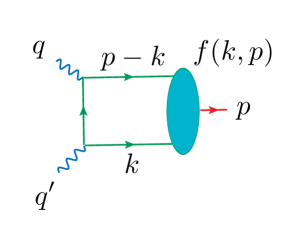
Figure 1: General handbag diagram for photon-pion transition form factor in momentum representation.

In the momentum representation, the hadron structure is described by the hadron-parton blob $f(k,p)$, which by Lorentz invariance depends on 3 variables: two parton virtuaities $k^{2}$, $(p-k)^{2}$, and the invariant mass $p^{2}$, which is $k$-independent. None of these invariants is convenient for extraction of the basic parton variable $x$ which is usually defined as the ratio $k^{+}/p^{+}$ of the “plus” light cone components.

A standard way to extract $k^{+}$ is to incorporate a light-like vector $n\equiv n^{-}$, which is additional to variables $k,p$ of the hadron-parton blob. Using the Sudakov parametrization $k=xp+\eta n+k_{\perp}$ [13] for the $\gamma\gamma^{*}\pi^{0}$ amplitude, it is convenient to take $n=q^{\prime}$, the momentum of the real photon. Another convention was used in the light-front approach of Ref. [4], where $n$ is not directly related to the momenta involved in the process (in particular, $q^{\prime}=p+n\,q_{\bot}^{2}/(2pn)-q_{\bot}$ in that definition).

Switching to the coordinate representation, one deals with the variable $z$ that is Fourier conjugate to $k$ (see Fig.2). The blob now depends on $p$ and $z$, and by Lorentz invariance is a function of $(pz)$ and $z^{2}$. Then the parton fraction $x$ may be defined just as a variable that is Fourier conjugate to $(pz)$. There is no need to have an external vector like $n$ in such a definition, which is truly process-independent and involves only a minimal set of vectors $p,z$ describing the hadron state under study.

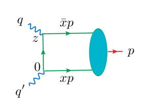
Figure 2: Handbag diagram in the coordinate representation and parton momentum assignment.

In the coordinate representation (see Fig. 2) we have

$$T(p,q)=\int{d^{4}z}\,e^{-i(qz)}\,D^{c}(z)\,\langle p|\phi(0)\phi(z)|0\rangle$$ (1)

for a scalar handbag diagram, where $D^{c}(z)=-i/4\pi^{2}z^{2}$ is the scalar massless propagator, $q$ is the momentum of the initial virtual “photon” ($q^{2}\equiv-Q^{2}$) given by $q=p-q^{\prime}$, with $p$ being the momentum of the final “pion”.

2.2 Twist decomposition of the bilocal operator

The pion structure is described by the matrix element $\langle p|\phi(0)\phi(z)|0\rangle$. To parametrize it, one may to wish to start with the Taylor expansion

$$\phi(z)=\sum_{n=0}^{\infty}\frac{1}{n!}\,z_{\mu_{1}}\ldots z_{\mu_{n}}\ {\partial}^{\mu_{1}}\ldots{\partial}^{\mu_{n}}\phi(0)\ .$$ (2)

The next step is to to write the tensor $z_{\mu_{1}}\ldots z_{\mu_{n}}$ as a sum of products of powers of $z^{2}$ and symmetric-traceless combinations $\{\ldots z_{\mu_{i}}\ldots z_{\mu_{j}}\ldots\}$ satisfying $g^{\mu_{i}\mu_{j}}\{\ldots z_{\mu_{i}}\ldots z_{\mu_{j}}\ldots\}=0$. Using the notation $\{z\partial\}^{n}\equiv\{z_{\mu_{1}}\ldots z_{\mu_{n}}\}\,\partial^{\mu_{1}}\ldots\partial^{\mu_{n}}$ for products of traceless tensors, we obtain

$$\phi(z)=\sum_{l=0}^{\infty}\left(\frac{z^{2}}{4}\right)^{l}\sum_{N=0}^{\infty}\frac{N+1}{l!(N+l+1)!}\{z{\partial}\}^{N}({\partial}^{2})^{l}\phi(0).$$ (3)

The operators containing powers of ${\partial}^{2}$ have higher twist, and their contribution to the light-cone expansion is accompanied by powers of $z^{2}$. Considering the lowest-twist term, one can write matrix elements of the local operators

$$\langle p|\phi(0)\{{\partial}^{\mu_{1}}\ldots{\partial}^{\mu_{n}}\}\phi(0)|0\rangle=i^{n}\sum_{k=0}^{n}A_{n}\,\{p^{\mu_{1}}\ldots\ldots p^{\mu_{n}}\}$$ (4)

in terms of the coefficients $A_{n}$. To perform summation over $n$, one can introduce the twist-2 distribution amplitude (DA) $\varphi(x)$ as a function whose $\bar{x}^{n}$ moments ($\bar{x}\equiv 1-x$) are related to $A_{n}$ by

$$\int_{0}^{1}\varphi(x)\,\bar{x}^{n}dx=A_{n}\ .$$ (5)

The calculation of the sum

$$\sum_{n=0}^{\infty}i^{n}\frac{\bar{x}^{n}}{n!}\,\{z_{\mu_{1}}\ldots z_{\mu_{n}}\}\,p^{\mu_{1}}\ldots\ldots p^{\mu_{n}}\equiv\sum_{n=0}^{\infty}i^{n}\frac{\bar{x}^{n}}{n!}\,\{zp\}^{n}\,$$ (6)

is complicated by traceless combinations $\{z_{\mu_{1}}\ldots z_{\mu_{n}}\}$. To this end, one can use the inverse expansion $\{zp\}^{n}=(zp)^{n}-\frac{1}{4}{(n-1)}\,z^{2}p^{2}(zp)^{n-2}+\ldots$ to obtain the parameterization

$$\langle p|\phi(0)\phi(z)|0\rangle=\int_{0}^{1}\varphi(x)\,\,e^{i\bar{x}(pz)}\,dx+{\cal O}(z^{2})$$ (7)

of the matrix element. The plane wave factor $e^{i\bar{x}(pz)}$ has a natural interpretation that the parton created at point $z$ carries the fraction $\bar{x}p$ of the pion momentum $p$.

The $(z^{2})^{k}$ terms brought in by the re-expansion of $\{zp\}^{n}$ are accompanied by $(p^{2})^{k}$ factors. These terms are purely kinematical, and may be summed explicitly, leading to an analog of Nachtmann [14, 2] corrections. To concentrate on dynamical effects, one may take $p^{2}=0$, in which case $\{zp\}^{n}=(zp)^{n}$, and summation over $n$ is straightforward.

2.3 Virtuality distributions

For a light-like momentum $p$, the ${\cal O}(z^{2})$ terms in Eq. (7) only come from the $(z^{2})^{l}$ terms of the original expansion (3) for $\phi(z)$. These terms are accompanied by matrix elements of higher-twist operators

$$\langle p|\phi(0)\{z{\partial}\}^{k}\left({\partial}^{2}\right)^{l}\phi(0)|0\rangle\equiv[i(zp)]^{k}\Lambda^{2l}A_{kl}\ .$$ (8)

The derivation above assumes that the matrix elements of operators containing high powers of ${\partial}^{2}$ are finite, with their size characterized by some scale $\Lambda$, which has an obvious meaning of typical virtuality of parton fields inside the hadron.

For $l=0$, the coefficients $A_{k0}\equiv A_{k}$ reduce to those defining the twist-2 DA $\varphi(x)$. In general, for each particular $l$, we can define the coefficients $A_{kl}$ to be proportional to the $\bar{x}^{k}$ moments of appropriate functions $\varphi_{l}(x)$, and arrive at parametrization

$$\langle p|\phi(0)\phi(z)|0\rangle= \sum_{l=0}^{\infty}\left(\frac{\Lambda^{2}z^{2}}{4}\right)^{l}\int_{0}^{1}dx\,\varphi_{l}(x)\,e^{i\bar{x}(pz)}$$

$$\equiv \int_{0}^{1}dx\,B(x,z^{2}/4)\,e^{i\bar{x}(pz)}$$ (9)

in terms of the bilocal function $B(x,z^{2}/4)$.

In fact, using the $\alpha$-representation as outlined in Refs. [15, 16, 17], it can be demonstrated that the contribution of any Feynman diagram to $\langle p|\phi(0)\phi(z)|0\rangle$ can be represented as

$$\langle p|\phi(0) \phi(z)|0\rangle=i^{l}\,\frac{P({\rm c.c.})}{(4\pi i)^{Ld/2}}\int_{0}^{\infty}\prod_{j=1}^{l}d\alpha_{j}[A(\alpha)+B(\alpha)]^{-d/2}$$

$$\times\exp\left\{-i\frac{z^{2}/4}{A(\alpha)+B(\alpha)}+i(pz)\frac{B(\alpha)}{A(\alpha)+B(\alpha)}\right\}$$

$$\times\exp\left\{ip^{2}C(\alpha)-i\sum_{j}\alpha_{j}(m_{j}^{2}-i\epsilon)\right\}\ ,$$ (10)

where $d$ is the space-time dimension, ${P({\rm c.c.})}$ is the relevant product of the coupling constants, $L$ is the number of loops of the diagram, $l$ is the number of its internal lines, and $A(\alpha),B(\alpha),C(\alpha)$ are positive functions of the $\alpha_{\sigma}$-parameters of the diagram. Thus, we can write the matrix element in the form

$$\langle p|\phi(0)\phi(z)|0\rangle= \int_{0}^{\infty}d\sigma\int_{0}^{1}dx\,\Phi(x,\sigma)\,\,e^{i\bar{x}(pz)-i\sigma{(z^{2}-i\epsilon)}/{4}}\,,$$ (11)

without any assumptions about regularity of the $z^{2}\to 0$ limit. There is also no need to assume that $p^{2}=0$.

In a formal Taylor expansion of $\phi(0)\phi(z)$ above, the $z^{2}$ factors are accompanied by $\partial^{2}$, thus the variable $\sigma$ is related to $\partial^{2}$, i.e., parton virtuality. For this reason, we will refer to the spectral function $\Phi(x,\sigma)$ as the virtuality distribution amplitude (VDA). One should be aware, though, that while the virtuality $k^{2}$ may be both positive and negative, $\sigma$ is a positive parameter.

The VDA $\Phi(x,\sigma)$ is related to the bilocal function $B(x,z^{2}/4)$ by a Laplace-type representation

$$B(x,\beta)=\int_{0}^{\infty}\,e^{-i\beta\sigma}\Phi(x,\sigma)\,d\sigma\ .$$ (12)

According to Eq. (10), $B(x,z^{2}/4)$ is a function of $z^{2}-i\epsilon$.

2.4 Transverse momentum distributions

The parton picture implies a frame in which $p$ has no transverse component, a large component in the “plus” direction and a small component in the “minus” direction, so as $p\to p^{+}$ when $p^{2}\to 0$. In the latter limit, only the “minus” component $z^{-}$ is essential in the product $(pz)$. In general, without assuming $p^{2}=0$, we can take a space-like separation $z$ having $z^{-}$ and $z_{\perp}$ components only (i.e., $z^{+}=0$), and introduce the impact parameter distribution amplitude (IDA) ${\varphi}(x,z_{\perp})\equiv B(x,-z_{\perp}^{2}/4)$,

$$\langle p|\phi(0)\phi(z)|0\rangle|_{z^{+}=0,p_{\perp}=0}=\int_{0}^{1}dx\,{\varphi}(x,z_{\perp})\,e^{i\bar{x}(pz^{-})}\ .$$ (13)

Note that $B(x,\beta)$ is defined both for positive and negative $\beta$, while ${\varphi}(x,z_{\perp})$ corresponds to negative $\beta$ only.

The IDA function may be also treated as a Fourier transform

$${\varphi}(x,z_{\perp})=\int{\Psi}(x,k_{\perp})\,e^{i(k_{\perp}z_{\perp})}\,{d^{2}k_{\perp}}$$ (14)

of the transverse momentum dependent distribution amplitude (TMDA) ${\Psi}(x,k_{\perp})$. TMDA can be written in terms of VDA as

$${\Psi}(x,k_{\perp})= \frac{i}{\pi}\int_{0}^{\infty}\frac{d\sigma}{\sigma}\,\Phi(x,\sigma)\,\,e^{-i(k_{\perp}^{2}-i\epsilon)/\sigma}\ .$$ (15)

Actually TMDA depends on $k_{\perp}^{2}$ only: ${\Psi}(x,k_{\perp})=\psi(x,k_{\perp}^{2})/\pi$.

This relation is quite general in the sense that it holds even if the $z^{2}\to 0$ limit for the matrix element $\langle p|\phi(0)\phi(z)|0\rangle$ of the bilocal operator is singular. However, if this limit is regular, then the coefficients of the Taylor series of $B(x,\beta)$ in $\beta$ are given by $\sigma$ moments of the VDA $\Phi(x,\sigma)$, which, in turn, are related to $k_{\perp}^{2}$ moments of TMDA ${\Psi}(x,k_{\perp})$, namely

$$\int{\Psi}(x,k_{\perp})\,k_{\perp}^{2n}\,d^{2}k_{\perp}=\frac{n!}{i^{n}}\int_{0}^{\infty}{\sigma}^{n}\,\Phi(x,\sigma)\,{d\sigma}\ .$$ (16)

For these moments to be finite, $\Phi(x,\sigma)$ should vanish for large $\sigma$ faster than any power of $1/\sigma$. The functions having this property will be sometimes referred to as “soft”. The lowest moment

$$\int_{0}^{\infty}\Phi(x,\sigma)\,d\sigma=\varphi(x)$$ (17)

of VDA $\Phi(x,\sigma)$ gives the usual twist-2 distribution amplitude $\varphi(x)$. The reduction relation for TMDA ${\Psi}(x,k_{\perp})$

$$\int{\Psi}(x,k_{\perp})\,d^{2}k_{\perp}=\varphi(x)$$ (18)

is equivalent to the reduction relation ${\varphi}(x,z_{\perp}=0)=\varphi(x)$ for the IDA ${\varphi}(x,z_{\perp})$. Using Eq. (16), we derive

$$B(x,\beta)=\int\Psi(x,k_{\perp})\,J_{0}(2k_{\perp}\sqrt{-\beta})\,d^{2}k_{\perp}\ .$$ (19)

For negative $\beta=-z_{\perp}^{2}/4$, this formula may be also obtained by performing the angular integration in Eq. (14). If $\beta$ is positive (then we can write $\beta=|z|^{2}/4$), one may understand Eq.(19) as

$$B(x,|z|^{2}/4)=\int\Psi(x,k_{\perp})\,I_{0}(k_{\perp}|z|)\,d^{2}k_{\perp}\ ,$$ (20)

where $I_{0}$ is the modified Bessel function. Thus, in some cases, the bilocal function $B(x,\beta)$ may be expressed in terms of TMDA $\Psi(x,k_{\perp})$ both for spacelike and timelike values of $\beta$. This fact suggests that it might be sufficient to know just the “spacelike” function $\Psi(x,k_{\perp})$ to describe all virtuality effects.

In our actual calculations, we have no need to separate integrations over spacelike and timelike $z$ and use Eqs. (19), (20) and/or the presumptions (like Taylor expansion in $z^{2}$) on which they are based. All the coordinate integrations are done covariantly, and furthermore, without any assumptions whether the $z^{2}\to 0$ limit for $B(x,z^{2}/4)$ is regular or not. The results are expressed in terms of VDA $\Phi(x,\sigma)$, and then Eq. (15) is incorporated that relates $\Phi(x,\sigma)$ to the TMDA $\Psi(x,k_{\perp})$. Our final expressions are given in terms of TMDA.

2.5 Handbag diagram in VDA representation

The strategy outlined above may be illustrated by calculation of the Compton amplitude. The starting expression is given by

$$T(p,q)=\int_{0}^{1}dx\int{d^{4}z}\,e^{i(q^{\prime}z)-ix(pz)}\,D^{c}(z)\,\,B(x,z^{2}/4)\ .$$ (21)

When the partons have zero virtuality, i.e. if all $\sigma^{l}$ moments with $l\geq 1$ vanish, we have $B(x,z^{2}/4)\Rightarrow\varphi(x)$. In this case, only the twist-2 operators contribute, and we have

$$T(p,q)|_{\rm twist\ 2}= -\int_{0}^{1}\frac{\varphi(x)\,dx}{(q^{\prime}-xp)^{2}+i\epsilon}$$

$$=\int_{0}^{1}\frac{\varphi(x)\,dx}{xQ^{2}+x\bar{x}p^{2}-i\epsilon}\ .$$ (22)

The $x\bar{x}p^{2}$ term here produces target-mass corrections analogous to those analyzed in Refs. [14, 2]. For positive $Q^{2}$ and $p^{2}$, the denominator has no singularities, and $i\epsilon$ may be omitted. Also, given the smallness of the pion mass, we will neglect $p^{2}$ in what follows. If necessary, the target mass corrections may be reconstructed by the appropriately made changes $xQ^{2}\to xQ^{2}+x\bar{x}m_{\pi}^{2}$ in the formulas given below.

To include the virtuality corrections, we use the VDA parametrization (11) that gives

$$T(Q^{2})= \int_{0}^{1}\frac{dx}{xQ^{2}}\,\int_{0}^{\infty}d\sigma\,{\Phi(x,\sigma)}\left\{1-e^{-[ixQ^{2}+\epsilon]/\sigma}\right\}\ .$$ (23)

The first term in the brackets does not depend on $\sigma$ and produces the twist-2 expression (22). Using the TMDA/VDA relation (15), one may rewrite Eq. (23) in terms of TMDA as

$$T(Q^{2})= \int_{0}^{1}\frac{dx}{xQ^{2}}\int_{k_{\perp}^{2}\leq{x}Q^{2}}\Psi(x,{k}_{\perp})\,d^{2}{k}_{\perp}\ .$$ (24)

2.6 TMDA and light-front wave function

One could notice that the definition of TMDA

$$\langle p|\phi(0)\phi(z)|0\rangle |_{z_{+}=0,p_{\perp}=0}=\int_{0}^{1}dx\,\,e^{i\bar{x}(pz_{-})}$$

$$\times\int{\Psi}(x,k_{\perp})\,e^{i(k_{\perp}z_{\perp})}\,{d^{2}k_{\perp}}$$ (25)

is similar to that for the light-front wave function used in Ref. [4]. The difference is that our approach is based on covariant calculations, with ${\Psi}(x,k_{\perp})$ appearing at final stages through its relation (15) to a covariant function $\Phi(x,\sigma)$ which is a generalization of the DA $\varphi(x)$. For this reason, we shall continue to use the “distribution amplitude” terminology for the VDA-related functions. In particular, ${\Psi}(x,k_{\perp})$ will be referred to as TMDA.

3 Spin-1/2 quarks

3.1 Non-gauge case

When quarks have spin 1/2, the handbag diagram for the pion transition form factor is given by

$$\int{d^{4}z}\,e^{-i(qz)}\langle p|\bar{\psi}(0) \gamma^{\nu}\,S^{c}(-z)\,\gamma^{\mu}\,\psi(z)|0\rangle=i\epsilon^{\mu\nu\alpha\beta}p_{\alpha}q_{\beta}F(Q^{2})\ ,$$ (26)

where $S^{c}(z)=\not{z}/2\pi^{2}(z^{2})^{2}$ is the propagator for a massless fermion. Using that the antisymmetric part of $\gamma^{\nu}\,\not{z}\,\gamma^{\mu}$ is $iz_{\beta}\epsilon^{\mu\nu\alpha\beta}\gamma_{5}\gamma_{\alpha}$ and writing the twist-2 part of the matrix element

$$\langle p|\bar{\psi}(0)\gamma_{5}\gamma_{\alpha}\,\psi(z)|0\rangle|_{\rm twist\ 2}\ =ip_{\alpha}\int_{0}^{1}dx\,e^{i\bar{x}(pz)}\,\,\varphi(x)$$ (27)

one obtains the same formula

$$F(Q^{2})|_{\rm twist\ 2}=\int_{0}^{1}\frac{\varphi(x)}{xQ^{2}}\,dx$$ (28)

as in the scalar model considered above. The higher-twist operators may be included through the VDA parametrization

$$\langle p|\bar{\psi}(0)\,\gamma_{5}\gamma_{\alpha}\,\psi(z)|0\rangle =ip_{\alpha}\int_{0}^{\infty}d\sigma\int_{0}^{1}dx\,$$

$$\times\Phi(x,\sigma)\,\,e^{i\bar{x}(pz)-i\sigma{(z^{2}-i\epsilon)}/{4}}+\ldots\ ,$$ (29)

in which we omitted the terms proportional to $z_{\alpha}$, since they disappear after convolution with $z_{\beta}\epsilon^{\mu\nu\alpha\beta}$. All the formulas relating VDA with IDA and TMDA that were derived in the scalar case are valid without changes. However, the spinor propagator has a different $\sim\not{z}/(z^{2})^{2}$ functional form. Using it, we obtain

$$F(Q^{2})= \int_{0}^{\infty}d\sigma\int_{0}^{1}{\Phi(x,\sigma)}\frac{dx}{xQ^{2}}\,\left\{1+\frac{i\sigma}{xQ^{2}}\left[1-e^{-[ixQ^{2}+\epsilon]/\sigma}\right]\right\}\ .$$ (30)

For large $Q^{2}$, Eq. (30) contains a power-like $\sim 1/Q^{4}$ correction that corresponds to the twist-4 $\bar{\psi}\gamma_{5}\gamma_{\alpha}D^{2}\psi$ operators. Though they are accompanied by a $z^{2}$ factor, the latter does not completely cancel the $1/z^{4}$ singularity of the spinor propagator, and this contribution has a “visible” $\Lambda^{2}/Q^{4}$ behavior. The remaining term contains contributions “invisible” in the OPE. In terms of TMDA we have

$$F(Q^{2})= \int_{0}^{1}\frac{dx}{xQ^{2}}\int_{0}^{xQ^{2}}\frac{dk_{\perp}^{2}}{xQ^{2}}\int_{{k^{\prime}_{\perp}}^{2}\leq k_{\perp}^{2}}\Psi(x,k^{\prime}_{\perp})\,d^{2}k^{\prime}_{\perp}\ .$$ (31)

With the help of Eq. (31), one can calculate form factor in various models for the TMDA $\Psi(x,{\kappa}_{\perp})$. Before analyzing form factor in some simple models for VDA, we show in the next section that switching to gauge theories does not bring any further changes in general equations.

3.2 Gauge theories

In gauge theories, the handbag contribution in a covariant gauge should be complemented by diagrams corresponding to operators $\bar{\psi}(0)\ldots A(z_{1})\ldots\psi(z)$ containing twist-0 gluonic field $A_{\mu}(z_{1})$ inserted into the fermion line between the points 0 and $z$ (see Fig. 3). It is well known [19, 20, 21] that these insertions may be organized to produce a path-ordered exponential

$${E}(0,z;A)\equiv P\exp{\left[ig\,z_{\mu}\,\int_{0}^{1}dt\,A^{\mu}(tz)\right]}$$ (32)

accumulating the zero-twist field $A^{\mu}$, and insertions of the non-zero twist gluon field

$${\mathfrak{A}}^{\mu}(z)=z_{\nu}\int_{0}^{1}\,G^{\mu\nu}(sz)\,s\,ds\ ,$$ (33)

which is the vector potential in the Fock-Schwinger gauge [22, 23]. These insertions correspond to three-body $\bar{q}Gq$, etc. higher Fock components. At the two-body $\bar{q}q$ Fock component level, we deal with the gauge-invariant bilocal operator

$${\cal O}^{\alpha}(0,z;A)\equiv\bar{\psi}(0)\,\gamma_{5}\gamma^{\alpha}\,{E}(0,z;A)\psi(z)\ .$$ (34)

An important property of this operator is that the Taylor expansion for ${\cal O}^{\alpha}(0,z;A)$ has precisely the same structure as that for the original $\bar{\psi}(0)\gamma_{5}\gamma^{\alpha}\psi(z)$ operator, with the only change that one should use covariant derivatives $D^{\mu}=\partial^{\mu}-igA^{\mu}$ instead of the ordinary $\partial^{\mu}$ ones:

$${E}(0,z;A)\,\psi(z)=\sum_{n=0}^{\infty}\frac{1}{n!}\,z_{\mu_{1}}\ldots z_{\mu_{n}}\ {D}^{\mu_{1}}\ldots{D}^{\mu_{n}}\psi(0)\ .$$ (35)

This means that one can introduce the parametrization

$$\langle p|\,{\cal O}^{\alpha}(0,z;A)|0\rangle= ip^{\alpha}\int_{0}^{\infty}d\sigma\int_{0}^{1}dx\,\Phi(x,\sigma)\,\,e^{i\bar{x}(pz)-i\sigma{(z^{2}-i\epsilon)}/{4}}$$

$$+z^{\alpha}\ldots$$ (36)

that accumulates information about higher twist terms in VDA $\Phi(x,\sigma)$ and proceed exactly like in a non-gauge case.

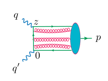
Figure 3: Structure of the handbag contribution in QCD.

4 Modeling soft transverse momentum dependence

To analyze predictions of the VDA approach for $F(Q^{2})$, we will use Eq. (31) incorporating there particular models for VDA $\Phi(x,\sigma)$ or TMDA $\Psi(x,k_{\perp})$. For illustration, we consider first the simplest case of factorized models $\Phi(x,\sigma)=\varphi(x)\,\Phi(\sigma)$ or

$$\Psi(x,k_{\perp})=\varphi(x)\,\psi(k_{\perp}^{2})\ ,$$ (37)

in which the $x$-dependence and $k_{\perp}$-dependence appear in separate factors, and later consider some non-factorized models.

4.1 Gaussian model

It is popular to assume a Gaussian dependence on $k_{\perp}$,

$$\Psi_{G}(x,k_{\perp})=\frac{\varphi(x)}{\pi\Lambda^{2}}e^{-k_{\perp}^{2}/\Lambda^{2}}\ .$$ (38)

In the impact parameter space, one gets IDA

$$\varphi_{G}(x,z_{\perp})={\varphi(x)}\,e^{-z_{\perp}^{2}\Lambda^{2}/4}$$ (39)

that also has a Gaussian dependence on $z_{\perp}$. Writing

$$\varphi_{G}(x,z_{\perp})= \frac{{\varphi(x)}}{2\pi}\int_{-\infty}^{\infty}\frac{i\,d\sigma}{\sigma+i\Lambda^{2}}\,\,e^{-iz_{\perp}^{2}\sigma/4}\ ,$$ (40)

we see that the integral involves both positive and negative $\sigma$, i.e. formally $\varphi_{G}(x,z_{\perp})$ cannot be written in the VDA representation (15). However, the form factor formula in terms of TMDA (31) shows no peculiarities in case of the Gaussian ansatz, so we will use this model because of its calculational simplicity.

4.2 Simple non-Gaussian models

One may also argue that the Gaussian ansatz (39) has too fast a fall-off for large $z_{\perp}$. For comparison, the propagator

$$D^{c}(z,m)=\frac{1}{16\pi^{2}}\int_{0}^{\infty}e^{-i\sigma z^{2}/4-i(m^{2}-i\epsilon)/\sigma}{d\sigma}$$ (41)

of a massive particle falls off as $\sim e^{-|z|m}$ for large space-like distances. At small $z^{2}$, however, the free particle propagator has $1/z^{2}$ singularity while we want a model for $\langle p|\phi(0)\phi(z)|0\rangle$ that is finite at $z=0$. The simplest way is to add a constant term $(-4/\Lambda^{2})$ to $z^{2}$ in the VDA representation (11). So, we take

$$\Phi(x,\sigma)=\frac{\varphi(x)}{p(\Lambda,m)}e^{i\sigma/\Lambda^{2}-im^{2}/\sigma-\epsilon\sigma}$$ (42)

as a model for VDA. The sign of the $\Lambda^{2}$ term is fixed from the requirement that $(4/\Lambda^{2}-z^{2})^{-1}$ should not have singularities for space-like $z^{2}$. The normalization factor $p(\Lambda,m)$ is given by

$${p(\Lambda,m)}=\int_{0}^{\infty}e^{i\sigma/\Lambda^{2}-im^{2}/\sigma-\epsilon\sigma}d\sigma=2i{m}{\Lambda}K_{1}(2m/\Lambda)\ .$$ (43)

4.3 $m=0$ models

To concentrate on the effects of introducing $\Lambda$, let us take $m=0$, i.e. consider

$$\Phi_{s}(x,\sigma)={\varphi(x)}\,\frac{e^{i\sigma/\Lambda^{2}-\epsilon\sigma}}{i\Lambda^{2}}\ .$$ (44)

The bilocal matrix element in this case is given by

$$\langle p|\phi(0)\phi(z)|0\rangle=\,\frac{1}{1-z^{2}\Lambda^{2}/4}\int_{0}^{1}dx\,{\varphi(x)}\,e^{ix(pz)}\,,$$ (45)

which corresponds to

$${\varphi}_{s}(x,z_{\perp})=\,\frac{\varphi(x)}{1+z_{\perp}^{2}\Lambda^{2}/4}$$ (46)

for IDA. Note that the $z_{\perp}^{2}$ term of the $z_{\perp}$ expansion of ${\varphi}(x,z_{\perp})$ in this model was adjusted to coincide with that of the exponential model, so that $\Lambda^{2}$ has the same meaning of the scale of $\phi\partial^{2}\phi$ operator. The TMDA for this ansatz is given by

$${\Psi}_{s}(x,k_{\perp})=2\varphi(x)\,\frac{K_{0}(2k_{\perp}/\Lambda)}{\pi\Lambda^{2}}\ .$$ (47)

It has a logarithmic singularity for small $k_{\perp}$ that reflects a slow $\sim 1/z_{\perp}^{2}$ fall-off of ${\varphi}_{s}(x,z_{\perp})$ for large $z_{\perp}$. The integrated TMDA that enters the form factor formula (31) is given by

$$\int_{{k^{\prime}}_{\perp}^{2}\leq k_{\perp}^{2}}\Psi(x,{k^{\prime}}_{\perp})\,d^{2}k^{\prime}_{\perp}=\varphi(x)\left[1-\frac{2k_{\perp}}{\Lambda}K_{1}(2k_{\perp}/\Lambda)\right]\ .$$ (48)

It is also possible to calculate explicitly the next $k_{\perp}$ integral involved there, see Eq. (56) below.

4.4 $m\neq 0$ model

The model with nonzero mass-like term

$$\Phi_{m}(x,\sigma)=\varphi(x)\frac{e^{i\sigma/\Lambda^{2}-im^{2}/\sigma}}{2i{m}{\Lambda}K_{1}(2m/\Lambda)}$$ (49)

corresponds to the function

$$\Psi_{m}(x,k_{\perp})=\varphi(x)\,\frac{K_{0}\left(2\sqrt{k_{\perp}^{2}+m^{2}}/\Lambda\right)}{\pi m\Lambda K_{1}(2m/\Lambda)}\ .$$ (50)

that is finite for $k_{\perp}=0$ in accordance with the fact that the IDA

$${\varphi}_{m}(x,z_{\perp})={\varphi(x)}\,\frac{K_{1}\left(m\sqrt{4/\Lambda^{2}+z_{\perp}^{2}}\,\right)}{K_{1}(2m/\Lambda)\,\sqrt{1+\Lambda^{2}z_{\perp}^{2}/4}}$$ (51)

in this case has $\sim e^{-m|z_{\perp}|}$ fall-off for large $z_{\perp}$. For small $z_{\perp}$, we have ${\varphi}_{m}(x,z_{\perp})={\varphi(x)}[1-z_{\perp}^{2}\tilde{\Lambda}^{2}(\Lambda,m)+\ldots]$ behavior.

5 Modeling transition form factor

Let us now use these models to calculate the transition form factor with the help of Eq.(31).

5.1 Gaussian model

In case of the Gaussian model (38), we have

$$F_{G}(Q^{2})= \int_{0}^{1}\frac{dx}{xQ^{2}}\,{\varphi(x)}\,\left[1-\frac{\Lambda^{2}}{xQ^{2}}\left(1-e^{-xQ^{2}/\Lambda^{2}}\right)\right]\ .$$ (52)

For large $Q^{2}$, Eq. (52) displays the power-like twist-4 contribution and the term that falls faster than any power of $1/Q^{2}$. Note that the $x$-integral for the purely twist-2 contribution converges if the pion DA $\varphi(x)$ vanishes as any positive power $x^{\alpha}$ for $x\to 0$, while the total integral in Eq. (52) converges even for singular DAs $\varphi(x)\sim x^{-1+\alpha}$ with arbitrarily small $\alpha$. Furthermore, the formal $Q^{2}\to 0$ limit is finite:

$$F_{G}(Q^{2}=0)=\frac{f_{\pi}}{2\Lambda^{2}}\ ,$$ (53)

where we have used the normalization condition

$$\int_{0}^{1}\varphi(x)\,dx=f_{\pi}\ .$$ (54)

Note that $F(Q^{2})$ is finite for $Q^{2}=0$ in any model with finite $\Psi(x,k_{\perp}=0)$. According to Eq. (31), one has then

$$F(Q^{2}=0)=\frac{\pi}{2}\int_{0}^{1}\Psi(x,k_{\perp}=0)\,dx\ .$$ (55)

5.2 $m=0$ model

Using the non-Gaussian model (44) with $m=0$ gives

$$F(Q^{2})= \int_{0}^{1}\frac{dx}{xQ^{2}}\,{\varphi(x)}\,\left[1-\frac{\Lambda^{2}}{xQ^{2}}+2K_{2}(2\sqrt{x}Q/\Lambda)\right]\ .$$ (56)

The size of the twist-4 term here is given by the confinement scale $\Lambda^{2}$, just as in the Gaussian model.

5.3 $m\neq 0$ model

Turning to the $m\neq 0$ model, we have

$$F_{m} (Q^{2})=\int_{0}^{1}\frac{dx}{xQ^{2}}\,{\varphi(x)}\,\left\{1-\frac{1}{xQ^{2}}\frac{\Lambda m}{K_{1}(2m/\Lambda)}\right.$$

$$\left.\times\left[K_{2}(2m/\Lambda)-\left(1+\frac{xQ^{2}}{m^{2}}\right)K_{2}(2{\sqrt{xQ^{2}+m^{2}}/\Lambda})\right]\right\}\ .$$ (57)

Now, the size of the twist-4 power correction depends on the interplay of the confinement scale $\Lambda$ and mass-type scale $m$.

5.4 Comparison with data

In QCD, the twist-2 approximation for $F(Q^{2})$ in the leading (zeroth) order in $\alpha_{s}$ is

$$F^{\rm LOpQCD}(Q^{2})= \int_{0}^{1}\frac{dx}{xQ^{2}}\,{\varphi(x)}\ .$$ (58)

Taking the value of $I(Q^{2})\equiv Q^{2}F(Q^{2})/f_{\pi}$ from the data gives information about the shape of the pion DA. In particular, for DAs of $\varphi_{r}(x)\sim(x\bar{x})^{r}$ type, one has $I_{r}^{\rm LOpQCD}(Q^{2})=1+2/r$, i.e. $I^{\rm as}(Q^{2})=3$ for the “asymptotic” wave function $\varphi^{\rm as}(x)=6f_{\pi}x\bar{x}$.

The most recent data [24, 25] still show a $Q^{2}$ variation of $I(Q^{2})$ (see Figs. 4, 5), especially in case of BaBar data [24] which contain several points with $I(Q^{2})$ values well above 3. It was argued [26, 27] that BaBar data indicate that the pion DA is close to a flat function $\varphi^{\rm flat}(x)=f_{\pi}$. The latter corresponds to $r=0$, and pQCD gives $I^{\rm flat}=\infty$. As shown in Ref. [26], inclusion of transverse momentum dependence of the pion wave function in the light-front formula of Ref. [4] (see also [8]) eliminates the divergence at $x=0$, and one can produce a curve that fits the BaBar data. Similar curves may be obtained within the VDA approach described in the present paper.

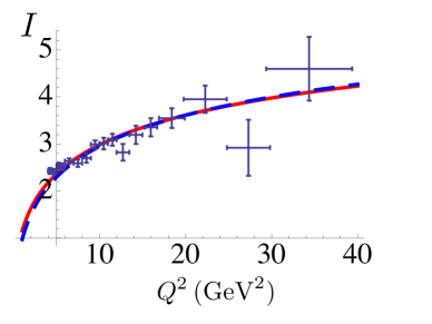
Figure 4: BABAR data compared to model curves described in the text.

In Fig. 4, we compare BaBar data with model curves corresponding to flat DA $\varphi(x)=f_{\pi}$ and two types of transverse momentum distributions. First, we take the Gaussian model of Eq. (52). A curve closely following the data is obtained for a value of $\Lambda^{2}=0.35\,$GeV² which is larger than the standard estimate $\Lambda^{2}=0.2\,$GeV² [18] for the matrix element of the $\bar{\psi}\gamma_{5}\gamma_{\alpha}D^{2}\psi$ operator. However, the higher-order pQCD corrections are known [28] to shrink the $z_{\perp}$ width of the IDA $\varphi(x,z_{\perp})$, effectively increasing the observed $\Lambda^{2}$ compared to the primordial value of $\Lambda^{2}$. For illustration, we also take the non-Gaussian $m=0$ model of Eq. (56), to check what happens in case of unrealistically slow $\sim 1/z_{\perp}^{2}$ decrease for large $z_{\perp}$. Still, if we take a larger value of $\Lambda^{2}=0.6\,$GeV², this model produces practically the same curve as the $\Lambda^{2}=0.35\,$GeV² Gaussian model.

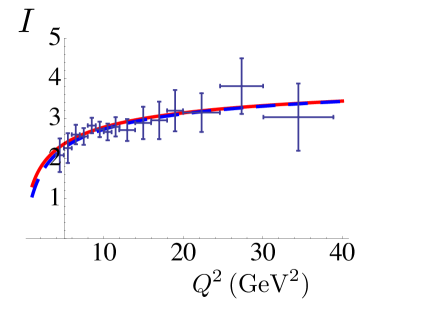
Figure 5: BELLE data compared to model curves described in the text.

Data from BELLE [25] give lower values for $I$, suggesting a non-flat DA. In Fig. 5, we show the curves corresponding to $\varphi(x)\sim f_{\pi}(x\bar{x})^{0.4}$ DA. If we take the Gaussian model (52), a good eye-ball fit to data is produced if we take $\Lambda^{2}=0.3\,$GeV². Practically the same curve is obtained in the non-Gaussian $m=0$ model of Eq. (56) for $\Lambda^{2}=0.4\,$GeV². Again, a VDA-based analysis of the higher-order Sudakov effects [28] is needed to extract the value of $\Lambda$ in the primordial TMDA.

6 Modeling hard tail

Higher-order pQCD corrections also modify the large-$k_{\perp}$ behavior of TMDA, producing a hard $\sim 1/k_{\perp}^{2}$ tail. Matching the soft and hard parts of transverse momentum distributions is a very important problem in their studies. Below, on simple scalar model examples we illustrate the basics of using the VDA approach for generation of hard tail terms from original purely soft distributions.

6.1 Simple model for hard TMDA

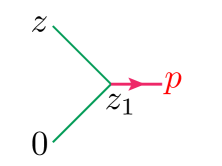
Figure 6: Modeling VDA by a local current source.

Modeling the matrix element $\langle p|\phi(0)\phi(z)|0\rangle$ by two propagators $D^{c}(z_{1},m)$ and $D^{c}(z-z_{1},m)$ (see Fig. 6), with momentum $p$ going out of the point $z_{1}$ gives (after integration over $z_{1}$)

$$\Phi^{\rm point}(x,\sigma)=\frac{1}{\sigma}\,e^{i(x\bar{x}p^{2}-m^{2})/\sigma}$$ (59)

for the analog of VDA. For TMDA, this yields

$$\Psi^{\rm point}(x,k_{\perp})=\frac{1}{\pi}\,\frac{1}{k_{\perp}^{2}+m^{2}-x\bar{x}p^{2}}\ .$$ (60)

It has a hard powerlike $1/k_{\perp}^{2}$ tail for large $k_{\perp}$. Making a formal $d^{2}k_{\perp}$ integration to produce DA, one faces in this case a logarithmic divergence. In the impact parameter space, we have $\varphi_{2}(x,z_{\perp})=2K_{0}(z_{\perp}\sqrt{m^{2}-x\bar{x}p^{2}})$, a function with a logarithmic singularity for $z_{\perp}=0$, which is another manifestation of the divergence of the $k_{\perp}$ integral for $\Psi_{2}(x,k_{\perp})$. In fact, the function $\Psi^{\rm point}(x,k_{\perp})$ has a “bound state” pole in $p^{2}$ at the location given by a well-known light-front combination $(k_{\perp}^{2}+m^{2})/x\bar{x}$. However, we see no reasons to expect that in general TMDAs $\Psi(x,k_{\perp})$ depend on $k_{\perp}$ through $k_{\perp}^{2}/x\bar{x}$.

6.2 Hard exchange model

A more complicated toy model involves two currents carrying momenta $yp$ and $(1-y)p\equiv\bar{y}p$ at locations $z_{1}$ and $z_{2}$, respectively (see Fig. 7).

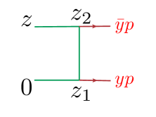
Figure 7: Modeling VDA by a two-current state.

With an exchange interaction described by a scalar propagator $D^{c}(z_{1}-z_{2},m)$, we have

$$\Phi^{\rm 2-curr}(x,\sigma;y)= ig^{2}\,\frac{e^{i(x\bar{x}p^{2}-m^{2})/\sigma}}{16\pi^{2}\,\sigma^{2}}\,\int_{0}^{{\rm min}\left\{\frac{x}{y},\,\frac{\bar{x}}{\bar{y}}\right\}}e^{-iy\bar{y}\beta\,{p^{2}}/{\sigma}}\,d\beta$$ (61)

as an analog of VDA, where $g$ is the coupling constant. For $p^{2}=0$, the $\beta$-integral gives a well-known combination

$$V(x,y)=\frac{x}{y}\,\theta(x<y)+\frac{\bar{x}}{\bar{y}}\,\theta(x>y)\ ,$$ (62)

that is a part of ERBL [10, 4] evolution kernel. For an analog of TMDA in the $p^{2}=0$ limit, we have

$$\Psi^{\rm 2-curr}(x,k_{\perp};y)=\frac{g^{2}}{16\pi^{3}}\frac{V(x,y)}{(k_{\perp}^{2}+m^{2})^{2}}\ .$$ (63)

A further step is a superposition model in which the $yp,\bar{y}p$ states enter with the weight $\varphi_{0}(y)$, a “primordial” distribution amplitude. Then the model TMDA is given by a convolution

$$\Psi^{\rm conv}(x,k_{\perp})=\frac{g^{2}}{16\pi^{3}}\,\frac{1}{(k_{\perp}^{2}+m^{2})^{2}}\int_{0}^{1}{V(x,y)}\,\varphi_{0}(y)\,dy\ .$$ (64)

The integral producing DA in this case converges to give $\varphi^{\rm conv}(x)={g^{2}}/{(8\pi^{2}m^{2})}\,\delta\varphi(x)$, where

$$\delta\varphi(x)\equiv[V\otimes\varphi_{0}]\,(x)=\int_{0}^{1}{V(x,y)}\,\varphi_{0}(y)\,dy\ ,$$ (65)

that has the meaning of a correction to $\varphi_{0}(x)$ generated by the simplest exchange interaction. However, the $k_{\perp}^{2}$ moment, and all higher $k_{\perp}^{2}$ moments of $\Psi^{\rm conv}(x,k_{\perp})$ diverge, which is reflected by $\ln z_{\perp}^{2}$ terms in the expansion of the relevant IDA

$$\varphi^{\rm conv}(x,z_{\perp})=mz_{\perp}K_{1}(mz_{\perp})\,\varphi^{\rm conv}(x)\ ,$$ (66)

since $aK_{1}(a)=1+aI_{1}(a)\ln a$ + analytic terms for small $a$.

6.3 Generating hard tail

Thus, an exchange of a “gluon” has converted a superposition of collinear (to $p$) “quark” states into a state that has $1/(k_{\perp}^{2}+m^{2})^{2}$ dependence on the transverse momentum $k_{\perp}$. We may also assume that the initial fields at $z_{1}$ and $z_{2}$ are described by some “primordial” bilocal function $B_{0}(y,(z_{1}-z_{2})^{2}/4)$ corresponding to a soft TMDA $\Psi_{0}(y,k_{\perp})\equiv\psi_{0}(x,k_{\perp}^{2})/\pi$ (see Fig. 8).

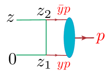
Figure 8: Hard tail model.

To concentrate on virtuality effects induced by $B_{0}$, we use $m=0$ and $p^{2}=0$. Then the generated hard TMDA is given by

$$\Psi^{B_{0}}(x,k_{\perp})= \frac{g^{2}}{16\pi^{3}k_{\perp}^{2}}\,\int_{0}^{1}dy\left[\int_{0}^{1}d\xi\,\psi_{0}\left(y,\frac{\xi k_{\perp}^{2}}{V(x,y}\right)\right]\ .$$ (67)

The term in square brackets may be written as

$$\Biggl{[}\cdots\Biggr{]}=\frac{V(x,y}{k_{\perp}^{2}}\left\{{\varphi_{0}(y)}-\int^{\infty}_{k_{\perp}^{2}/V(x,y)}\psi_{0}(y,{k^{\prime}_{\perp}}^{2})\,d{k^{\prime}_{\perp}}^{2}\right\}\ ,$$ (68)

where $\varphi_{0}(y)$ is the primordial distribution $\Psi_{0}(y,k^{\prime}_{\perp})$ integrated over all the transverse momentum plane. Hence, for large $k_{\perp}$, the leading $1/k_{\perp}^{4}$ term is determined by the DA $\varphi_{0}(y)$ only. A particular shape of the $k_{\perp}$-dependence of the soft TMDA $\Psi_{0}(y,k_{\perp})$ affects only the subleading $\sim[V\otimes\psi_{0}](x,k_{\perp}^{2})/k_{\perp}^{2}$ term. The form of $k_{\perp}$ dependence of $\Psi_{0}(y,k_{\perp})$ is also essential for the behavior of $\Psi^{B_{0}}(x,k_{\perp})$ term at small $k_{\perp}$. In particular, we have

$$\Biggl{[}\cdots\Biggr{]}_{k_{\perp}=0}=\psi_{0}(y,k_{\perp}^{2}=0)\ ,$$ (69)

which gives, e.g., $\varphi_{0}(y)/\Lambda^{2}$ in the Gaussian model (38).

6.4 Hard tail for spin-1/2 quarks

In case of spin-1/2 quarks interacting $via$ a (pseudo)scalar gluon field (“Yukawa” gluon model), Eq. (67) is modified by an extra $k_{\perp}^{2}$ factor coming from the numerator spinor trace, which leads to $1/(k_{\perp}^{2}+m^{2})$ dependence in the correction (64) to the TMDA. It results in a $\varphi^{\rm conv}_{Y}(x,z_{\perp})\sim K_{0}(mz_{\perp})\,\delta\varphi(x)$ term for the IDA. The logarithmic divergence for $z_{\perp}=0$ of this outcome corresponds to evolution of the DA. In the $B_{0}$ model, we have (switching to $\varphi(x,z_{\perp})\to\varphi(x,z_{\perp}^{2})$ in our notations below)

$$\varphi^{B_{0}}_{Y}(x,z_{\perp}^{2})= \frac{g^{2}}{16\pi^{2}}\int_{0}^{1}dy\,V(x,y)\int_{1}^{\infty}\frac{d\nu}{\nu}\,\varphi_{0}\Bigl{(}y,\nu\,z_{\perp}^{2}\,V(x,y)\Bigr{)}\ .$$ (70)

Substituting formally $\varphi_{0}(y,z_{\perp}^{2})$ by $\varphi_{0}(y)$ in the $z_{\perp}^{2}\to 0$ limit, we get a logarithmically divergent integral over $\nu$. In fact, for a function $\varphi_{0}(y,z_{\perp}^{2})$ that rapidly decreases when $z_{\perp}^{2}\gtrsim 1/\Lambda^{2}$, one gets $\ln(z_{\perp}^{2}\Lambda^{2})$ as a factor accompanying the convolution of $V(x,y)$ and $\varphi_{0}(y)$. Hence, the pion size cut-off contained in the primordial distribution provides the scale in $\log(z_{\perp}^{2})$, and we may keep the hard quark propagators massless. This cut-off also results in a finite value of $\Psi^{B_{0}}_{Y}$ in the formal $k_{\perp}\to 0$ limit:

$$\Psi^{B_{0}}_{Y}(x,k_{\perp}=0)= \frac{g^{2}}{16\pi^{2}}\,\int_{0}^{1}dy\,\Psi_{0}\left(y,k_{\perp}=0\right)\ .$$ (71)

Thus, the $\Psi^{\rm conv}_{Y}(x,k_{\perp})\sim\delta\varphi(x)/k_{\perp}^{2}$ singularity of the “collinear model” $\Psi_{0}(y,k_{\perp})=\varphi_{0}(y)\,\delta(k_{\perp}^{2})/\pi$ converts into a constant $1/\Lambda^{2}$ in the Gaussian model. Note also that the overall factor in Eq. (71) then contains the $x$-independent integral of $\varphi_{0}(y)$, i.e. $f_{\pi}$, rather than the convolution $\delta\varphi(x)$ as in Eq. (64).

Concluding, we emphasize that the VDA approach provides an unambiguous prescription of generating hard-tail terms like $\Psi^{B_{0}}(x,k_{\perp})$ from a soft primordial distribution $\Psi_{0}(y,k_{\perp})$. A subject for future studies is to use this strategy for building hard tail models in case of QCD.

7 Summary and outlook

In the present paper, we outlined a new approach to transverse momentum dependence in hard processes. Its starting point, just like in the OPE formalism, is the use of coordinate representation. At handbag level, the structure of a hadron with momentum $p$ is described by a matrix element of the bilocal operator ${\cal O}(0,z)$, treated as a function of $(pz)$ and $z^{2}$. It is parametrized through a virtuality distribution $\Phi(x,\sigma)$, in which the variable $x$ is Fourier-conjugate to $(pz)$, and has the usual meaning of a parton momentum fraction. Another parameter, $\sigma$, is conjugate to $z^{2}$ through an analog of Laplace transform.

Projecting ${\cal O}(0,z)$ onto a spacelike interval with $z^{+}=0$, we introduce transverse momentum distributions $\Psi(x,k_{\perp})$ and show that they can be written in terms of virtuality distributions $\Phi(x,\sigma)$. This fact opens the possibility to convert the results of covariant calculations, written in terms of $\Phi(x,\sigma)$, into expressions involving $\Psi(x,k_{\perp})$. This procedure being a crucial feature of our approach, is illustrated in the present paper by its application to hard exclusive transition process $\gamma^{*}\gamma\to\pi^{0}$ at the handbag level (which is analogous to the 2-body Fock state approximation). Starting with scalar toy models, we then extend the analysis onto the case of spin-1/2 quarks and vector gluons.

We propose a few simple models for soft VDAs/TMDAs, and use them for comparison of VDA results with experimental (BaBar and BELLE) data on the pion transition form factor.

A natural next step is going beyond the handbag approximation. In QCD, an important feature is that quark-gluon interactions generate a hard $\sim 1/k_{\perp}^{2}$ tail for TMDAs. To demonstrate the capabilities of the VDA approach in this direction, we describe the basic elements of generating hard tails from soft primordial TMDAs.

Another direction for future studies is an extension of the VDA approach onto inclusive reactions, such as Drell-Yan and SIDIS processes. In particular, we envisage building VDA-based models for soft parts of TMDs that would have a non-Gaussian behavior at large $k_{\perp}$ (the need for such models was recently emphasized by several authors [29, 30, 31]). The VDA approach would also allow to self-consistently generate hard tails from these soft TMDs.

References

• [1] P. J. Mulders and R. D. Tangerman, Nucl. Phys. B 461, 197 (1996)
• [2] H. Georgi and H. D. Politzer, Phys. Rev. D 14, 1829 (1976).
• [3] A. V. Efremov and A. V. Radyushkin, Lett. Nuovo Cim.  19, 83 (1977).
• [4] G. P. Lepage and S. J. Brodsky, Phys. Rev. D 22, 2157 (1980).
• [5] F. del Aguila and M. K. Chase, Nucl. Phys. B 193, 517 (1981).
• [6] E. Braaten, Phys. Rev. D 28, 524 (1983).
• [7] E. P. Kadantseva, S. V. Mikhailov and A. V. Radyushkin, Yad. Fiz.  44, 507 (1986) [ Sov. J. Nucl. Phys.  44, 326 (1986)].
• [8] I. V. Musatov and A. V. Radyushkin, Phys. Rev. D 56, 2713 (1997)
• [9] A. V. Radyushkin, JINR report P2-10717 (unpublished);hep-ph/0410276 (English translation) (1977)
• [10] A. V. Efremov and A. V. Radyushkin, Phys. Lett. B 94, 245 (1980).
• [11] V. L. Chernyak, A. R. Zhitnitsky and V. G. Serbo, JETP Lett.  26, 594 (1977) [Pisma Zh. Eksp. Teor. Fiz.  26, 760 (1977)].
• [12] G. P. Lepage and S. J. Brodsky, Phys. Lett. B 87, 359 (1979).
• [13] V. V. Sudakov, Sov. Phys. JETP 3, 65 (1956)
• [14] O. Nachtmann, Nucl. Phys. B 63, 237 (1973).
• [15] A. V. Radyushkin, Phys. Lett. B 131, 179 (1983).
• [16] A. V. Radyushkin, Theor. Math. Phys.  61, 1144 (1985)
• [17] A. V. Radyushkin, Phys. Rev. D 56, 5524 (1997)
• [18] V. A. Novikov, M. A. Shifman, A. I. Vainshtein, M. B. Voloshin and V. I. Zakharov, Nucl. Phys. B 237, 525 (1984).
• [19] A. V. Efremov and A. V. Radyushkin, JINR-E2-11535 (1978).
• [20] A. V. Efremov and A. V. Radyushkin, Theor. Math. Phys.  44, 774 (1981)
• [21] A. V. Efremov and A. V. Radyushkin, Riv. Nuovo Cim.  3N2, 1 (1980).
• [22] V. Fock, Sowjet. Phys. 12, p. 404 (1937).
• [23] J. S. Schwinger, Phys. Rev.  82, 664 (1951).
• [24] B. Aubert et al. [BaBar Collaboration], Phys. Rev. D 80, 052002 (2009)
• [25] S. Uehara et al. [Belle Collaboration], Phys. Rev. D 86, 092007 (2012)
• [26] A. V. Radyushkin, Phys. Rev. D 80, 094009 (2009)
• [27] M. V. Polyakov, JETP Lett.  90, 228 (2009)
• [28] H. -n. Li and G. F. Sterman, Nucl. Phys. B 381, 129 (1992).
• [29] J. Collins, Int. J. Mod. Phys. Conf. Ser.  25, 1460001 (2014)
• [30] D. Sivers, Int. J. Mod. Phys. Conf. Ser.  25, 1460002 (2014)
• [31] P. Schweitzer, M. Strikman and C. Weiss, JHEP 1301, 163 (2013) .