Observability of thermal effects in the Casimir interaction from graphene-coated substrates

Abstract

Using the recently proposed theory, we calculate thermal effect in the Casimir interaction from graphene-coated metallic and dielectric substrates. The cases when only one or both of the two parallel plates are coated with graphene are considered. It is shown that the graphene coating does not influence the Casimir interaction between metals, but produces large impact for dielectrics. This impact increases with decreasing static dielectric permittivity of the plate material. The thermal correction to the gradient of the Casimir force between an Au sphere and graphene coated fused silica plate is calculated. It is shown to be significanlty greater than the total experimental error in the recently performed experiment, which is demonstrated to be only one step away from observation of the thermal effect from a graphene-coated substrate at short separation distances. To achieve this goal, one should increase the thickness of the fused silica film from 300 nm to $2\,\mu$m.

I Introduction

Thermal effects in the Casimir interaction have been the subject of much attention (see Ref. 1 for a review). However, until the present day they are not observed at short separations of the order of 100 nm, i.e., in the region characterized by the highest experimental precision. In this respect such unusual material as graphene, which is a 2D sheet of carbon atoms, is of special interest. As was shown in Ref. 2 , for graphene the thermal effects become crucial at much shorter separations than for ordinary materials. This result was obtained by using the longitudinal density-density correlation function and later reconfirmed within quantum electrodynamical formalism of the polarization tensor in (2+1)-dimensional space-time 3 ; 4 . In doing so, graphene was described in the framework of the Dirac model 5 which is applicable at low energies below several eV, as appropriate for fluctuation-induced van der Waals and Casimir forces. Later on, a lot of calculations of graphene-graphene, graphene-plate, and atom-graphene Casimir and Casimir-Polder interactions has been performed using different methods 6 ; 7 ; 8 ; 9 ; 10 ; 11 ; 12 ; 13 ; 14 ; 15 ; 16 .

Measurements of the Casimir force between two freestanding graphene sheets or between a graphene sheet and a material plate present a real challenge due to deformations of graphene surfaces. Because of this, in the pioneering experiment 17 it was chosen to measure the gradient of the Casimir force between an Au-coated sphere and a graphene sheet deposited on a SiO₂ film covering a Si plate. Measurements were performed using a dynamic atomic force microscope (AFM) operated in the frequency shift mode 17 . However, the comparison of the measurement data with theory was made difficult because the available reflection coefficients for graphene deposited on a substrate 18 ; 19 ; 20 were expressed in terms of the dielectric permittivity of substrate material and the density-density correlation functions of graphene. The main difficulty encounted in computations was that the expression for the transverse density-density correlation function, as well as the explicit temperature-dependence of both longitudinal and transverse functions, remained unknown. In these conditions, Ref. 17 used the additive theory which overestimates the force gradient, and, as a consequence, only a qualitative agreement with the experimental data was achieved.

The state of affairs has been changed only recently due to two important results obtained in the literature. In Ref. 21 , an explicit connection between the density-density correlation functions and the components of the polarization tensor was established. In the process, the analytic expression for the transverse correlation function and the temperature dependence of both longitudinal and transverse functions have been found. Furthermore, in Ref. 22 the reflection coefficients for a graphene sheet deposited on a substrate were derived independently in terms of the dielectric permittivity of a substrate material and the polarization tensor of graphene. The results of Refs. 21 ; 22 were found to be in agreement. On this basis the experimental data of Ref. 17 were compared with the proposed theory and a very good quantitative agreement was demonstrated within the limits of the experimental errors. This raises a question as to whether thermal effects in Casimir interaction between graphene-coated substrates are observable using the existing laboratory setup.

In this paper, we calculate the thermal Casimir pressure between metallic and dielectric substrates coated with graphene. The cases when only one or both two material plates are coated with a graphene sheet are considered. We perform computations for gold, silicon, sapphire, mica and fused silica substrates. It is shown that the role of graphene is the most pronounced for a substrate material having the smallest static dielectric permittivity (fused silica in our case). For metallic substrates the deposition of a graphene sheet does not lead to a detectable change in the Casimir pressure. Then we calculate the thermal correction to the gradient of the Casimir force between an Au sphere and a SiO₂ plate coated with a graphene sheet at the experimental separations of a few hundred nanometers. It is shown that over a sufficiently wide region of separations the thermal correction is up to a factor of 5 larger than the total experimental error. Finally, we demonstrate that the experiment of Ref. 17 , which was the pioneer measurement of the Casimir interaction with a graphene-coated substrate, was only one step away from measuring the respective thermal effect as well. According to our results, the latter goal can be achieved if to increase the thickness of SiO₂ film in Ref. 17 from 300 nm to $2\,\mu$m.

The paper is organized as follows. In Sec. II we briefly present the Lifshitz formula for graphene-coated substrates where the reflection coefficients are expressed in terms of the dielectric permittivity and the polarization tensor. The influence of graphene films on the thermal Casimir pressure between material plates is analyzed in Sec. III. In Sec. IV the thermal effect in the gradient of the Casimir force between an Au-coated sphere and a SiO₂ plate is calculated and the possibility to observe it is demonstrated. Section V contains our conclusions and discussion.

II The Lifshitz formula for graphene-coated substrates

In this section we consider the thermal Casimir pressure $P(a,T)$ between two thick plates (semispaces) separated by a distance $a$ at least one of which is coated with a graphene sheet. The Lifshitz formula in terms of the reflection coefficients takes the standard form 23 ; 24

$$P(a,T)=-\frac{k_{B}T}{8\pi a^{3}}\sum_{l=0}^{\infty}{\vphantom{\sum}}^{\prime}\int_{\zeta_{l}}^{\infty}\!\!y^{2}dy\left[\frac{R_{\rm TM}^{(1)}(i\zeta_{l},y)R_{\rm TM}^{(2)}(i\zeta_{l},y)}{e^{y}-R_{\rm TM}^{(1)}(i\zeta_{l},y)R_{\rm TM}^{(2)}(i\zeta_{l},y)}\right.$$

$$~{}~{}~{}~{}~{}~{}\left.+\frac{R_{\rm TE}^{(1)}(i\zeta_{l},y)R_{\rm TE}^{(2)}(i\zeta_{l},y)}{e^{y}-R_{\rm TE}^{(1)}(i\zeta_{l},y)R_{\rm TE}^{(2)}(i\zeta_{l},y)}\right].$$ (1)

Here, $k_{B}$ is the Boltzmann constant, $T$ is the temperature, and the dimensionless Matsubara frequencies $\zeta_{l}$ are expressed via the dimensional ones by $\zeta_{l}=2a\xi_{l}/c$, where $\xi_{l}=2\pi k_{B}Tl/\hbar$ with $l=0,\,1,\,2,\,\ldots$ (the prime on the summation sign indicates that the term with $l=0$ is divided by two). Note that the dimensionless variable $y$ is connected by the equation

$$y=2aq_{l}\equiv 2a\left(k_{\bot}^{2}+\frac{\xi_{l}^{2}}{c^{2}}\right)^{1/2}$$ (2)

with the projection of the wave vector on the plane of plates $k_{\bot}$.

The reflection coefficients on the graphene-coated substrates were found by different methods in Refs. 18 ; 19 ; 20 combined with Ref. 21 , on the one hand, and in Ref. 22 , on the other hand. They are given by

$$R_{\rm TM}^{(n)}(i\zeta_{l},y)=\frac{\varepsilon_{l}^{(n)}y+k_{l}^{(n)}\left(\frac{y}{y^{2}-\zeta_{l}^{2}}\tilde{\Pi}_{00}-1\right)}{\varepsilon_{l}^{(n)}y+k_{l}^{(n)}\left(\frac{y}{y^{2}-\zeta_{l}^{2}}\tilde{\Pi}_{00}+1\right)},$$

(3)

$$R_{\rm TE}^{(n)}(i\zeta_{l},y)=\frac{y-k_{l}^{(n)}-\left(\tilde{\Pi}_{\rm tr}-\frac{y^{2}}{y^{2}-\zeta_{l}^{2}}\tilde{\Pi}_{00}\right)}{y+k_{l}^{(n)}+\left(\tilde{\Pi}_{\rm tr}-\frac{y^{2}}{y^{2}-\zeta_{l}^{2}}\tilde{\Pi}_{00}\right)},$$

where the dielectric permittivities for the materials of the first and second semispaces ($n=1,\,2$) are

$$\varepsilon_{l}^{(n)}\equiv\varepsilon^{(n)}(i\xi_{l})=\varepsilon^{(n)}(ic\zeta_{l}/2a),$$ (4)

$\tilde{\Pi}_{00}$ is the 00-component, $\tilde{\Pi}_{\rm tr}$ is the sum of spatial components $\tilde{\Pi}_{1}^{\,1}$ and $\tilde{\Pi}_{2}^{\,2}$ of the dimensionless polarization tensor in (2+1)-dimensional space time 3 ; 4 , and the following notation is introduced

$$k_{l}^{(n)}\equiv\sqrt{y^{2}+(\varepsilon_{l}^{(n)}-1)\zeta_{l}^{2}}.$$ (5)

The dimensionless components are connected with the dimensional ones by the equations

$$\tilde{\Pi}_{00}\equiv\tilde{\Pi}_{00}(i\zeta_{l},y)=\frac{2a}{\hbar}\Pi_{00},\qquad\tilde{\Pi}_{\rm tr}\equiv\tilde{\Pi}_{\rm tr}(i\zeta_{l},y)=\frac{2a}{\hbar}\Pi_{\rm tr}.$$ (6)

Now we present analytic expressions for the components of the polarization tensor entering Eq. (3). This tensor depends on $T$ both explicitly as on a parameter and implicitly through the Matsubara frequencies. It was shown 4 ; 10 ; 12 ; 13 that an explicit dependence on $T$ substantially affects the computational results for the Casimir free energy and pressure only through the zero-frequency term of the Lifshitz formula $l=0$. In so doing, all terms of Eq. (1) with $l\geq 1$ without the loss of accuracy can be calculated using the polarization tensor defined at $T=0$ and depending on $T$ only implicitly.

The respective exact expressions at $\zeta_{0}=0$ for a graphene with a nonzero mass gap parameter $\Delta$ are 4 ; 10

$$\tilde{\Pi}_{00}(0,y)=\frac{8\alpha}{\tilde{v}_{F}^{2}}\left[\frac{\tau}{\pi}\int_{0}^{1}\!\!dx\ln\left(2\cosh\frac{\pi\theta}{\tau}\right)-\tilde{\Delta}^{\!2}\int_{0}^{1}\frac{dx}{\theta}\tanh\frac{\pi\theta}{\tau}\right],$$ (7)

$$\tilde{\Pi}_{\rm tr}(0,y)-\tilde{\Pi}_{00}(0,y)=8\alpha\tilde{v}_{F}^{2}y^{2}\!\int_{0}^{1}\!\!\!dx\frac{x(1-x)}{\theta}\tanh\frac{\pi\theta}{\tau}.$$

Here, $\alpha=e^{2}/(\hbar c)$ is the fine-structure constant, $\tilde{v}_{F}=v_{F}/c$, where $v_{F}\approx 9\times 10^{5}\,$m/s is the Fermi velocity in graphene 25 ; 26 , $\tau\equiv 4\pi ak_{B}T/(\hbar c)$ is the temperature parameter, $\tilde{\Delta}\equiv 2a\Delta/(\hbar c)$, and the function $\theta$ is defined as

$$\theta\equiv\theta(x,y)=[\tilde{\Delta}^{\!2}+x(1-x)\tilde{v}_{F}^{2}y^{2}]^{1/2}.$$ (8)

It is seen that the right-hand sides in Eq. (7) depend on $T$ explicitly through the dimensionless parameter $\tau$.

At all Matsubara frequencies $\zeta_{l}$ with $l\geq 1$ one can use the following expressions for the components of the polarization tensor at $T=0$, where the continuous $\zeta$ are replaced with the discrete $\zeta_{l}$ 3 ; 4 ; 10 :

$$\tilde{\Pi}_{00}(i\zeta_{l},y)=\alpha\frac{y^{2}-\zeta_{l}^{2}}{f^{2}(\zeta_{l},y)}\,\Phi(\zeta_{l},y),$$ (9)

$$\tilde{\Pi}_{\rm tr}(i\zeta_{l},y)-\frac{y^{2}}{y^{2}-\zeta_{l}^{2}}\tilde{\Pi}_{00}(i\zeta_{l},y)=\alpha\Phi(\zeta_{l},y),$$

where the functions $\Phi$ and $f$ are given by

$$f(\zeta_{l},y)=[\tilde{v}_{F}^{2}y^{2}+(1-\tilde{v}_{F}^{2})\zeta_{l}^{2}]^{1/2},$$ (10)

$$\Phi(\zeta_{l},y)=4\tilde{\Delta}+2f(\zeta_{l},y)\left[1-\frac{4\tilde{\Delta}^{\!2}}{f^{2}(\zeta_{l},y)}\right]\arctan\frac{f(\zeta_{l},y)}{2\tilde{\Delta}}.$$

The reflection coefficients between thick plates (semispaces) made of ordinary materials with no graphene coatings are obtained from Eq. (3) by putting $\tilde{\Pi}_{00}=\tilde{\Pi}_{\rm tr}=0$. If the graphene coating is missing on only one plate, $n=2$, for instance, the polarization tensor should be put equal to zero only in these specific reflection coefficients $R_{\rm TM}^{(2)}$ and $R_{\rm TE}^{(2)}$.

III Influence of graphene coatings on the thermal Casimir pressure

In this section we calculate the influence of graphene coatings on the Casimir pressure at $T=300\,$K for plates (semispaces) made of various materials, both metallic and dielectric, using the Lifshitz formula (1) and the reflection coefficients (3). For the sake of simplicity, here we consider the case of pristine (gapless) graphene because at $T=300\,$K the allowable nonzero mass gap parameters ($\Delta<0.1\,$eV 3 ) lead to only minor deviations in the magnitudes of the thermal Casimir force, as compared to the case $\Delta=0$ 10 . In Sec. IV the influence of nonzero mass gap parameter is specified in more detail.

We examine the case when both plates are made of a common material, so that $\varepsilon_{l}^{(1)}=\varepsilon_{l}^{(2)}$, and either one of them or both two are coated with a graphene sheet. As the first example, we consider Au plates. The dielectric permittivity of Au at the imaginary Matsubara frequencies is obtained by means of the Kramers-Kronig relation from the tabulated optical data 27 extrapolated down to zero frequency 1 ; 24 . Computations show that the values of the ratios $P_{g}/P$ and $P_{gg}/P$, where $P_{g}$ and $P_{gg}$ are the Casimir pressures between two Au plates one of which or both two are coated with graphene, respectively, and $P$ is the pressure between uncoated plates, do not depend on the type of extrapolation of the optical data by means of the Drude or the plasma model. The values of the plasma frequency $\omega_{p}=9.0\,$eV and the relaxation parameter $\gamma=0.035\,$eV have been used in extrapolations.

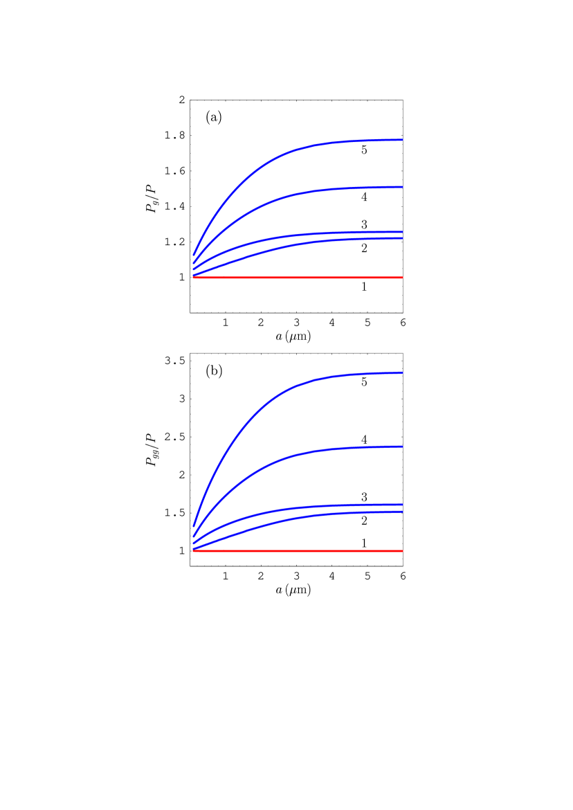
Figure 1: (Color online) Ratios of the Casimir pressures between two plates (a) one of which is coated with graphene and (b) both are coated with graphene to the Casimir pressure between uncoated plates are shown as functions of separation. The lines numbered 1, 2, 3, 4, and 5 are for plate materials Au, Si, sapphire, mica, and fused silica, respectively

The computational results for the ratios $P_{g}/P$ and $P_{gg}/P$ are shown by the lines numbered 1 in Fig. 1(a) and Fig. 1(b), respectively, as functions of separation. As can be seen in these figures, the Casimir pressure between Au plates is scarcely affected by graphene coatings over the wide range of separations from 100 nm to $6\,\mu$m. As an illustration, at $a=100\,$nm we have $P_{g}/P=1.0013$ and $P_{gg}/P=1.0025$, and both ratios quickly decrease to unity with increasing separation. The same holds for any metal or even for a doped semiconductor in a metallic state (i.e., for the concentration of charge carriers above the critical value). Thus, for B-doped Si (the concentration of charge carriers $n\approx 1.6\times 10^{19}\,\mbox{cm}^{-3}$) at $a=100\,$nm one obtains $P_{g}/P=1.0041$ and $P_{gg}/P=1.0082$, i.e., the maximum influence of graphene coatings is less than 1%.

To obtain the larger influence of graphene coatings on the Casimir pressure, we consider substrates made of different dielectric materials, such as high-resistivity Si, sapphire (Al₂O₃), mica, and fused silica (SiO₂) possessing the static dielectric permittivities $\varepsilon(0)$ equal to 11.7, 10.1, 5.4, and 3.8, respectively. The dielectric permittivity of Si along the imaginary frequency axis was obtained from the tabulated optical data 28 by means of the Kramers-Kronig relation. As to sapphire, mica, and fused silica, the available sufficiently precise analytic representations for their frequency-dependent dielectric permittivities have been used 29 .

The computational results for the ratios $P_{g}/P$ and $P_{gg}/P$ as functions of separation are shown in Fig. 1(a) and Fig. 1(b), respectively, by the lines 2 (high-resistivity Si), 3 (sapphire), 4 (mica), and 5 (fused silica). As is seen in Fig. 1, for dielectric plates the presence of graphene coatings significantly influences the Casimir pressure. This influence is larger when both dielectric plates are coated with graphene comparing to the case when only one plate is graphene-coated. It is significant that influence of graphene coatings on the Casimir pressure increases with decreasing static dielectric permittivity of the substrate material. This is the case for both one and two plates coated with graphene. From Fig. 1 we conclude that the largest impact of graphene coatings on the Casimir pressure takes place for the fused silica substrate. Thus, when one of the two fused silica plates is coated with graphene we have $P_{g}/P=1.17$, 1.25, 1.43, and 1.78 at separation distances $a=200\,$nm, 400 nm, $1\,\mu$m, and $6\,\mu$m, respectively. For two graphene-coated fused silica plates $P_{gg}/P=1.47$, 1.72, 2.28, and 3.34 at the same respective separations. Thus, for dielectric substrates the influence of graphene coatings can be sufficiently large even at short separation distances below $1\,\mu$m, i.e., in the measurement region of precise experiments on measuring the Casimir interaction (see Ref. 1 and more recent experiments 17 ; 30 ; 31 ; 32 ; 33 ).

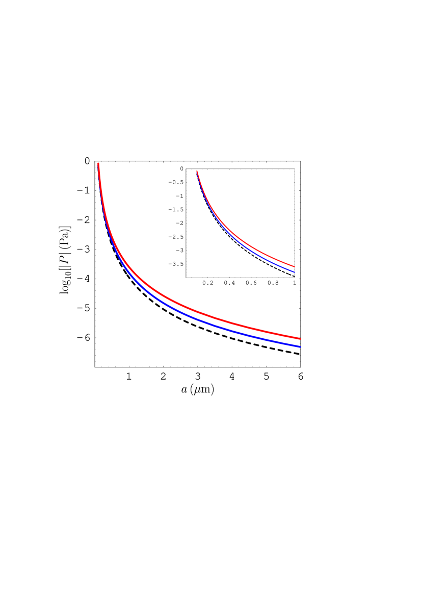
Figure 2: (Color online) Magnitudes of the Casimir pressure between two fused silica plates (dashed line), between one graphene-coated and one uncoated (the lower solid line), and between two graphene-coated fused silica plates (the upper solid line) are plotted as functions of separation. The separation region from 100 nm to $1\,\mu$m is shown on an inset.

To understand the absolute value of the calculated effects, in Fig. 2 we plot as functions of separation the magnitudes of the Casimir pressure between two fused silica plates (the dashed line), between one graphene-coated and one uncoated (the lower solid line) and between two graphene-coated fused silica plates (the upper solid line). For better visualization, the separation region from 100 nm to $1\,\mu$m is shown on an inset. As can be seen in Fig. 2, the presence of graphene layers essentially changes the magnitudes of the Casimir pressure both at short and long separation distances. Taking into account that the thermal effect in graphene is a special case, this can be used for its observation in measuring the Casimir interaction between graphene-coated substrates. We consider this possibility in the next section.

IV Possibility to observe the thermal effect in Casimir interaction with graphene-coated substrates

Precise measurements of the Casimir interaction mentioned above were performed in the configuration of a sphere of radius $R$ above a plane plate. The separation distance between the sphere and the plate was always much smaller than $R$, i.e., the inequality $a\ll R$ was satisfied with a wide safety margin. Thus, the comparison of the measurement data with theory can be performed using the proximity force approximation (PFA) stating that the Casimir force between the sphere and the plate is given by 1 ; 24

$$F_{\!\!sp}(a,T)=2\pi R{\cal F}(a,T),$$ (11)

where ${\cal F}(a,T)$ is the free energy of the Casimir interaction between two parallel plates per unit area. Calculating the negative derivative of Eq. (11) with respect to $a$, one obtains a connection between the measured force gradient in sphere-plate geometry and the effective Casimir pressure between two parallel plates

$$\frac{F_{\!\!sp}^{\prime}(a,T)}{R}=-2\pi P(a,T).$$ (12)

Note that using the exact theory of the Casimir interaction, applicable to boundary surfaces of arbitrary shape, the relative error of Eq. (12) was shown to be smaller than $(0.3\div 0.4)a/R$ 34 ; 35 ; 36 ; 37 .

Now we consider the proposed experimental configuration of an Au-coated sphere and a graphene-coated plate made of SiO₂, which is a substrate leading to the largest influence of graphene coating (see Sec. III). Although according to the results of Sec. III the coating of both test bodies by graphene influences the Casimir pressure even stronger, this option is not feasible experimentally because the second body is of spherical shape.

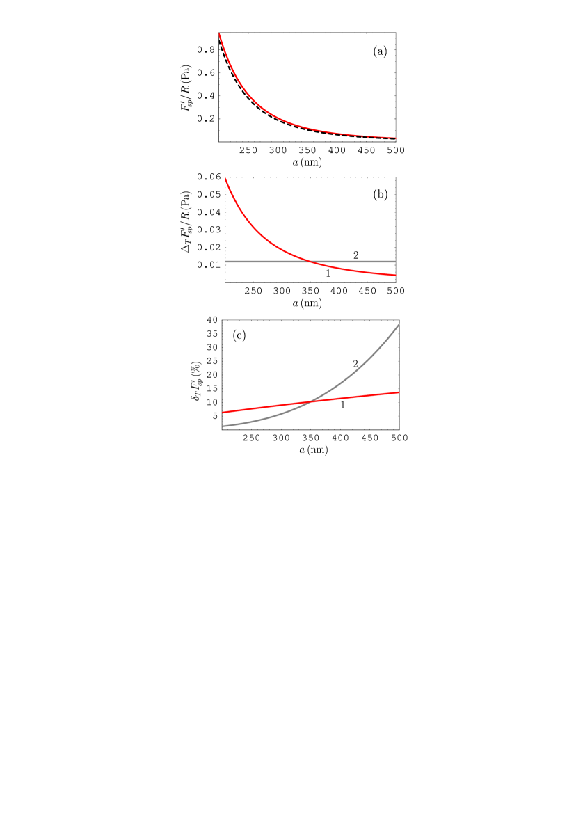
Figure 3: (Color online) (a) The normalized gradient of the Casimir force between an Au sphere of radius R and a graphene-coated SiO₂ plate at $T=300\,$K and $T=0\,$K are shown by the solid and dashed lines, respectively. The lines numbered 1 indicate (b) the absolute and (c) the relative thermal correction to the normalized force gradient. For comparison purposes, the lines numbered 2 show (b) the absolute and (c) the relative total experimental errors in the experiment 17 .

We have computed the quantity $F_{\!\!sp}^{\prime}/R$ for an Au sphere interacting with a graphene-coated SiO₂ plate using Eqs. (1) and (12). The reflection coefficients $R_{\rm TM,TE}^{(1)}$ in Eq. (3) are calculated with the dielectric permittivity $\varepsilon_{l}^{(1)}$ of SiO₂ and the polarization tensor of graphene. The reflection coefficients $R_{\rm TM,TE}^{(2)}$ are calculated with the dielectric permittivity $\varepsilon_{l}^{(2)}$ of Au and $\tilde{\Pi}_{00}=\tilde{\Pi}_{\rm tr}=0$. The type of extrapolation of the optical data for Au to zero frequency leads to only a minor influence on the computational results 10 . The computations were performed at $T=300\,$K and at $T=0\,$K. In the latter case the summation in Eq. (1) was replaced with an integration over continuous frequency 24 . The computational results as functions of separation are shown in Fig. 3(a) by the solid and dashed lines for $T=300\,$K and at $T=0\,$K, respectively.

The thermal correction to the force gradient normalized by $R$,

$$\frac{1}{R}{\Delta_{T}F_{\!\!sp}^{\prime}(a)}\equiv\frac{1}{R}\left[F_{\!\!sp}^{\prime}(a,T=300\,\mbox{K})-F_{\!\!sp}^{\prime}(a,T=0\,\mbox{K})\right],$$ (13)

is shown by the line 1 in Fig. 3b as a function of separation. The solid line 2 indicates the value of the total experimental error in measurements of the normalized force gradient in the experiment of Ref. 17 equal to 0.012 Pa. As is seen in Fig. 3(b), the thermal correction markedly exceeds the total experimental error at separations below 350 nm. In Fig. 3(c), the relative thermal correction

$$\delta_{T}F_{\!\!sp}^{\prime}(a)=\frac{\Delta_{T}F_{\!\!sp}^{\prime}(a)}{F_{\!\!sp}^{\prime}(a,T=300\,\mbox{K})}$$ (14)

is shown by the line 1 as a function of separation. In the same figure the solid line 2 indicates the relative error in measurements of the force gradient. It is again seen that the thermal effect due to the graphene coating of the SiO₂ plate is observable using the parameters of already existing laboratory setup 17 .

Now we discuss whether the thermal correction due to graphene sheet deposited on a substrate was observed in the experiment of Ref. 17 . In this experiment, the gradient of the Casimir force was measured between an Au-coated sphere of $R=54.1\,\mu$m radius and a graphene sheet deposited on a SiO₂ film of thickness $D=300\,$nm covering a B-doped Si plate of thickness $500\,\mu$m. The latter can be considered as a semispace. As was mentioned in Sec. I, in Ref. 22 the measurement data of Ref. 17 were compared with the theory describing graphene-coated substrates and a very good agreement was found. This comparison was performed at the laboratory temperature $T=300\,$K. The computations at $T=0\,$K were not performed, and the possibility to observe the thermal effect was not discussed.

The gradient of the Casimir force at $T=0$ can be computed using Eqs. (12) and (1). In the latter the discrete summation should be replaced with an integration over continuous frequency. The reflection coefficients $R_{\rm TM,TE}^{(2)}$ on an Au semispace are expressed as discussed above. The reflection coefficients $R_{\rm TM,TE}^{(g,f,s)}$ on a graphene sheet deposited on a SiO₂ film covering Si semispace, which should be used instead of $R_{\rm TM,TE}^{(1)}$ in Eq. (1), are expressed by using the standard formulas of the Lifshitz theory for planar layered structures 24 ; 38 ; 39

$$R_{\rm TM,TE}^{(g,f,s)}(i\zeta,y)=\frac{R_{\rm TM,TE}^{(1)}(i\zeta,y)+r_{\rm TM,TE}^{(f,s)}(i\zeta,y)e^{-2Dk_{f}^{(1)}}}{1+R_{\rm TM,TE}^{(1)}(i\zeta,y)r_{\rm TM,TE}^{(f,s)}(i\zeta,y)e^{-2Dk_{f}^{(1)}}}.$$ (15)

Here, the coefficients $R_{\rm TM,TE}^{(1)}$ describe the reflection on a graphene sheet deposited on a SiO₂ semispace. They are given in Eq. (3) where $\varepsilon^{(1)}\equiv\varepsilon_{f}^{(1)}$ is the dielectric permittivity of SiO₂ along the imaginary frequency axis. The coefficients $r_{\rm TM,TE}^{(f,s)}$ are well known Fresnel coeffisients. They describe the reflection on the boundary between two semispaces made of SiO₂ and Si

$$r_{\rm TM}^{(f,s)}(i\zeta,y)=\frac{\varepsilon_{s}^{(1)}k_{f}^{(1)}-\varepsilon_{f}^{(1)}k_{s}^{(1)}}{\varepsilon_{s}^{(1)}k_{f}^{(1)}+\varepsilon_{f}^{(1)}k_{s}^{(1)}},\qquad r_{\rm TE}^{(f,s)}(i\zeta,y)=\frac{k_{f}^{(1)}-k_{s}^{(1)}}{k_{f}^{(1)}+k_{s}^{(1)}}.$$ (16)

The quantity $\varepsilon_{s}^{(1)}$ is the dielectric permittivity of Si calculated along the imaginary frequency axis, and $k_{s}^{(1)}$, $k_{f}^{(1)}$ are defined in Eq. (5) and calculated with respective dielectric permittivities $\varepsilon_{s}^{(1)}$ and $\varepsilon_{f}^{(1)}$.

In Fig. 4 the measurement data of Ref. 17 are indicated as crosses. The arms of the crosses show the errors in the measured separation distances and force gradients determined at the 67% confidence level. The results of theoretical computations made in Ref. 22 at $T=300\,$K using the proposed theory describing graphene-coated substrates are shown as the light-gray band. The width of the band is determined by the uncertainty in the plasma frequency of metallic Si used in Ref. 17 , differences between the predictions of the Drude and plasma model extrapolations of the optical data of Au and Si to zero frequency, and by the uncertainty of the mass gap parameter of graphene within the interval from 0 to 0.1 eV. In the same figure, our computational results at $T=0\,$K are presented by the dark-gray band. The larger thickness of this band is explained by the fact that the influence of nonzero mass gap parameter $\Delta$ on the computational results is stronger at $T=0\,$K. Note that the results of computations at both $T=300\,$K and $T=0\,$K were corrected for the presence of surface roughness measured by means of AFM. This correction, however, was found to be below 0.1% of the calculated force gradients. As can be seen in Fig. 4, the computational results at $T=300\,$K are in a very good agreement with the measurement data, whereas the computations using the same theory, but performed at $T=0\,$K, deviate from the data by touching them only slightly. This means that the experiment of Ref. 17 was only one step away from measuring the thermal effect between an Au sphere and a graphene coated substrate. According to our resulys, the single point in this experiment which needs to be revised is the increased up to $2\,\mu$m thickness of the SiO₂ film. We have checked by means of numerical computations that in this case the SiO₂ film below graphene can be already considered as a semispace, and the underlying Si plate has no detrimental effect by decreasing the thermal correction to the measured force gradient.

V Conclusions and discussion

In this paper we have investigated the thermal effect in the Casimir interaction between graphene-coated substrates using the recently proposed theory. The thermal Casimir pressure as a function of separatiom was calculated when only one or both of the two parallel plates are coated with a graphene sheet. As the plate materials, we have considered Au or other metals and also different dielectrics (dielectric silicon, sapphire, mica and fused silica). It was shown that the graphene coating of metallic substrate does not influence the thermal Casimir pressure. For dielectric materials the influence of graphene coating is shown to increase with decreasing static dielectric permittivity of substrate material. Thus, among the materials mentioned above, we have the largest impact of graphene coating on the Casimir pressure in the case of fused silica.

Furthermore, we have calculated both the absolute and relative thermal corrections to the gradient of the Casimir force between an Au sphere and graphene-coated fused silica plate, which is the configuration of recent experiment 17 . According to our result, at separations below 350 nm the magnitude of the thermal correction up to a factor of 5 exceeds the total experimental error in the measured force gradient. This means that, when employing the appropriate substrate material, it is possible to observe the thermal effect from deposition of graphene sheet by using the already existing experimental setup.

Finally, we have calculated the zero-temperature gradient of the Casimir force in the experiment 17 , i.e., between an Au sphere and a graphene sheet deposited on a SiO₂ film covering a Si plate. It was shown that the computational results at $T=0\,$K deviate from the measurement data by touching them only slightly. The same data are in a very good agreement with the computational results at $T=300\,$K 22 . It is concluded that the experiment 17 was only one step away from measuring the thermal effect from graphene deposited on a SiO₂ substrate. To achieve this goal, it would be necessary to increase the thickness of a SiO₂ film from 300 nm to $2\,\mu$m.

To conclude, we have shown that thermal effects in the Casimir interaction from graphene-coated substrates are observable at short separations below $1\,\mu$m, where the highest experimental precision is achieved.

         

         

     

                          

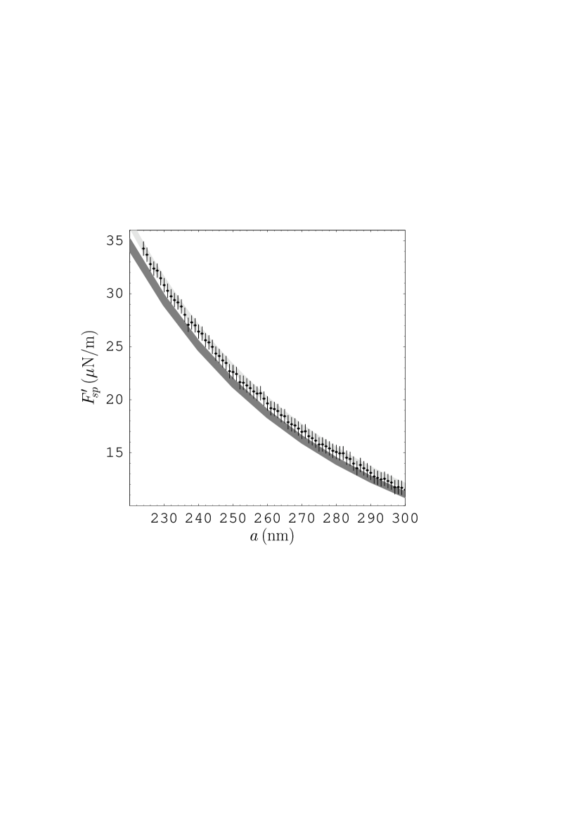
Figure 4: The measured gradients of the Casimir force between an Au-coated sphere and graphene deposited on a SiO₂ film covering a Si plate are indicated as crosses at different separations. The computational results at $T=300\,$K and $T=0\,$K are shown by the light-gray and dark-gray bands, respectively. See text for further discussion.

References

- (1) G. L. Klimchitskaya, U. Mohideen, and V. M. Mostepanenko, Rev. Mod. Phys. 81, 1827 (2009).
- (2) G. Gómes-Santos, Phys. Rev. B 80, 245424 (2009).
- (3) M. Bordag, I. V. Fialkovsky, D. M. Gitman, and D. V. Vassilevich, Phys. Rev. B 80, 245406 (2009).
- (4) I. V. Fialkovsky, V. N. Marachevsky, and D. V. Vassilevich, Phys. Rev. B 84, 035446 (2011).
- (5) A. H. Castro Neto, F. Guinea, N. M. R. Peres, K. S. Novoselov, and A. K. Geim, Rev. Mod. Phys. 81, 109 (2009).
- (6) D. Drosdoff and L. M. Woods, Phys. Rev. B 82, 155459 (2010).
- (7) Bo E. Sernelius, Europhys. Lett. 95, 57003 (2011).
- (8) D. Drosdoff and L. M. Woods, Phys. Rev. A 84, 062501 (2011).
- (9) T. E. Judd, R. G. Scott, A. M. Martin, B. Kaczmarek, and T. M. Fromhold, New. J. Phys. 13, 083020 (2011).
- (10) M. Bordag, G. L. Klimchitskaya, and V. M. Mostepanenko, Phys. Rev. B 86, 165429 (2012).
- (11) A. D. Phan, L. M. Woods, D. Drosdoff, I. V. Bondarev, and N. A. Viet, Appl. Phys. Lett. 101, 113118 (2012).
- (12) M. Chaichian, G. L. Klimchitskaya, V. M. Mostepanenko, and A. Tureanu, Phys. Rev. A 86, 012515 (2012).
- (13) G. L. Klimchitskaya and V. M. Mostepanenko, Phys. Rev. B 87, 075439 (2013).
- (14) S. Ribeiro and S. Scheel, Phys. Rev. A 88, 042519 (2013).
- (15) G. L. Klimchitskaya and V. M. Mostepanenko, Phys. Rev. A 89, 012516 (2014).
- (16) G. L. Klimchitskaya and V. M. Mostepanenko, Phys. Rev. B 89, 035407 (2014).
- (17) A. A. Banishev, H. Wen, J. Xu, R. K. Kawakami, G. L. Klimchitskaya, V. M. Mostepanenko, and U. Mohideen, Phys. Rev. B 87, 205433 (2013).
- (18) L. A. Falkovsky and S. S. Pershoguba, Phys. Rev. B 76, 153410 (2007).
- (19) T. Stauber, N. M. R. Peres, and A. K. Geim, Phys. Rev. B 78, 085432 (2008).
- (20) Bo E. Sernelius, Phys. Rev. B 85, 195427 (2012).
- (21) G. L. Klimchitskaya, V. M. Mostepanenko, and Bo E. Sernelius, Phys Rev. B 89, 125407 (2014).
- (22) G. L. Klimchitskaya, U. Mohideen, and V. M. Mostepanenko, Phys. Rev. B 89, 115419 (2014).
- (23) E. M. Lifshitz and L. P. Pitaevskii, Statistical Physics, Pt.II (Pergamon Press, Oxford, 1980).
- (24) M. Bordag, G. L. Klimchitskaya, U. Mohideen, and V. M. Mostepanenko, Advances in the Casimir Effect (Oxford University Press, Oxford, 2009).
- (25) B. Wunsch, T. Stauber, F. Sols, and F. Guinea, New J. Phys. 8, 318 (2006).
- (26) N. M. R. Peres, F. Guinea, and A. H. Castro Neto, Phys. Rev. B 73, 125411 (2006).
- (27) Handbook of Optical Constants of Solids, ed. E. D. Palik (Academic, New York, 1985).
- (28) Handbook of Optical Constants of Solids, vol II, ed. E. D. Palik (Academic, New York, 1991).
- (29) L. Bergström, Adv. Colloid Interface Sci. 70, 125 (1997).
- (30) C.-C. Chang, A. A. Banishev, R. Castillo-Garza, G. L. Klimchitskaya, V. M. Mostepanenko, and U. Mohideen, Phys. Rev. B 85, 165443 (2012).
- (31) A. A. Banishev, C.-C. Chang, G. L. Klimchitskaya, V. M. Mostepanenko, and U. Mohideen, Phys. Rev. B 85, 195422 (2012).
- (32) A. A. Banishev, G. L. Klimchitskaya, V. M. Mostepanenko, and U. Mohideen, Phys. Rev. Lett. 110, 137401 (2013).
- (33) A. A. Banishev, G. L. Klimchitskaya, V. M. Mostepanenko, and U. Mohideen, Phys. Rev. B 88, 155410 (2013).
- (34) C. D. Fosco, F. C. Lombardo, and F. D. Mazzitelli, Phys. Rev. D 84, 105031 (2011).
- (35) G. Bimonte, T. Emig, R. L. Jaffe, and M. Kardar, Europhys. Lett. 97, 50001 (2012).
- (36) G. Bimonte, T. Emig, and M. Kardar, Appl. Phys. Lett. 100, 074110 (2012).
- (37) L. P. Teo, Phys. Rev. D 88, 045019 (2013).
- (38) M. S. Tomaš, Phys. Rev. A 66, 052103 (2002).
- (39) G. L. Klimchitskaya, U. Mohideen, and V. M. Mostepanenko, J. Phys.: Condens. Matter 24, 424202 (2012).