Channel Selection for Network-assisted D2D Communication via No-Regret Bandit Learning with Calibrated Forecasting

Abstract

We consider the distributed channel selection problem in the context of device-to-device (D2D) communication as an underlay to a cellular network. Underlaid D2D users communicate directly by utilizing the cellular spectrum but their decisions are not governed by any centralized controller. Selfish D2D users that compete for access to the resources construct a distributed system, where the transmission performance depends on channel availability and quality. This information, however, is difficult to acquire. Moreover, the adverse effects of D2D users on cellular transmissions should be minimized. In order to overcome these limitations, we propose a network-assisted distributed channel selection approach in which D2D users are only allowed to use vacant cellular channels. This scenario is modeled as a multi-player multi-armed bandit game with side information, for which a distributed algorithmic solution is proposed. The solution is a combination of no-regret learning and calibrated forecasting, and can be applied to a broad class of multi-player stochastic learning problems, in addition to the formulated channel selection problem. Analytically, it is established that this approach not only yields vanishing regret (in comparison to the global optimal solution), but also guarantees that the empirical joint frequencies of the game converge to the set of correlated equilibria.

I Introduction

I-A Related Works

D2D communication underlying cellular networks enables wireless devices to communicate directly instead of through an access point or a base station (BS), provided that such transmissions do not disturb prioritized cellular transmissions [1]. This concept has been proposed to (i) boost the overall network efficiency expressed in terms of radio resources, and (ii) to provide users with more reliable services at lower costs [2].
Similar to other wireless networking scenarios, spectrum resource management is a key component of D2D communication systems, and may be studied within two different frameworks. The first framework, adapted by [3], [4] and [5] among many others, considers D2D and cellular systems as the two parts of a single entity with resources allocated by some BS, which is assumed to be in possession of global channel and network knowledge. The second framework, in contrast, considers a hierarchical relationship, where cellular and D2D systems are regarded as primary and secondary systems, respectively, and the resource allocation for the D2D system is performed in a distributed manner. This viewpoint can be found some literatures including [6], [7], [8] and [9].
Since conventional pilot signals cannot be used for estimation of D2D channels, the assumption of precise D2D channel information availability at some BS is not realistic. As a result, we argue in favor of the second framework described before, and we assume that D2D users establish a secondary distributed network that is allowed to use vacant spectrum resources of cellular network, thereby causing no interference to primary users. In this context, a vast majority of schemes, including those proposed by papers mentioned above, have some game-theoretical basis. Most of the game-theoretical models, however, require that the players know at least their own utility function. Moreover, statistical knowledge on channel gains and/or traffic model should be available. If not, they either require heavy information exchange among users (buyer-seller market models [10], cooperative game models [11]), and/or a coordinator (auctions [12]). In addition, since game-theoretical framework (cooperative or non-cooperative) requires all game parties to be known by each other, provision of required information is extremely costly. In order to address these shortcomings, one approach is to incorporate learning theory, as performed in the context of cognitive radio networks. Some works, for instance [13], [14] and [15], consider single-agent learning scenarios, while others study opportunistic spectrum access in multi-agent learning setting. In such setting, agents have access to strictly limited or even no information, and the objective is to satisfy some optimality condition. In what follows, we discuss some of these works in more details.

In [16], opportunistic spectrum access is formulated as a multi-agent learning game. In this work, it is assumed that upon availability, each channel pays the same reward to all users. This assumption, however, is strictly restrictive as it neglects channel qualities. On the other hand, if a channel is selected by multiple users, orthogonal spectrum access is applied, and therefore interference is neglected. In [17] and [18], authors consider the interference minimization game for partially overlapping channels. In these works, it is assumed that interference emerge only between neighboring users, and the proposed learning approaches are based on graphical games. In addition, in the three works mentioned above, the designed game is proven to be an exact potential game so that a pure-strategy Nash equilibrium exists. It can be thus concluded that the generalization of proposed approaches as well as convergence analyses is not straightforward. In [19], two approaches are proposed to achieve Nash equilibrium in a multi-player cognitive environment. System verification, however, is only based on numerical approaches. Other examples are [20], [21] and [22]. In these works, channel qualities are taken into account; nonetheless, it is assumed that in case of collision, no reward is paid to colliding users. Thus, interference is again neglected. Moreover, in the proposed algorithms, learning and channel selection are two independent procedures; while the former follows multi-armed bandit scenario, the latter is formulated as bipartite graph matching. This decoupling yields unnecessary complexity, and it is also not clear whether the final solution is stable or not, which is the main concern of equilibrium. The works [23], [24] and [25] propose various selection schemes to achieve logarithmic regret as well as fairness among users. However, equilibrium analysis is absent.

I-B Our Contribution

In this paper, we study a multi-player adaptive decision making problem, where selfish players learn the optimal action from successive interactions with a dynamic environment, and finally settle at some equilibrium point. This problem appears in many wireless networking scenarios, with a particular instance being the channel selection in a distributed D2D communication system integrated into a centralized cellular network. In our setting, each D2D user is selfish and aims at optimizing its throughput performance, while being allowed to use vacant cellular channels. We model this problem as a multi-armed bandit game among multiple learning agents that are provided with no prior information about channel quality and availability. We propose a channel selection strategy that consists of two main blocks, namely calibrated forecasting ([26], [27], [28]) and no-regret bandit learning ([29], [30], [31], [32]). Whereas calibrated forecasting is utilized to predict the joint action profile of selfish rational players, no-regret learning builds a trust-worthy estimate of the reward generating processes of arms. We show that our proposed model and selection strategy can be applied to both noise-limited (orthogonal channel access) and interference-limited (non-orthogonal channel access) transmission models. We prove that the gap between the average utility achieved by our approach and that of the optimal fixed strategy converges to zero as the game horizon tends to infinity. Moreover, by using our strategy, the empirical joint frequencies of play converge to the set of correlated equilibria.
As discussed in Section I-A, the spectrum access problem using learning theory has been under extensive study in recent years. Nevertheless, our work differs from previous studies in many aspects, as listed briefly in the following.

• Some works such as [13] and [14] analyze single-agent learning problem. In some others such as [20] and [21], although multi-agent problem is formulated, no explicit equilibrium analysis is performed. We, however, propose an algorithmic solution for multi-agent learning and show that by applying our approach the empirical joint frequencies of the game converge to the set of correlated equilibria. As any Nash equilibrium belongs to the set of correlated equilibria, our solution is more general in comparison to approaches that converge to a pure-strategy Nash equilibrium, for example those proposed in [16], [17], [18] and [19].

• The proposed multi-player learning approach can be applied to solve a wide range of resource allocation problem, including radio resource management, routing, scheduling, object tracking and so on. This is due to the fact that our convergence analysis does not depend on utility or cost function. In contrast, References [16], [17] and [18] require the game be an exact potential game for an equilibrium to be achieved by proposed approaches, and hence the applicability of these approaches is strictly restricted.

• In our problem setting, both noise-limited and interference-limited transmission models are studied, and do not impose any limitation on the interference pattern. This is in contrast with [21], [17] and [18], where the interference is either completely neglected or is limited to neighboring users. This is important since depending on channel matrices, channel allocation based on interference avoidance might be suboptimal.

• In our work, channels (or generally, actions) differ for different users. More precisely, variations in both channel availability and quality is taken into account. This stands in contrast to [16], where the average gain of each specific channel is assumed to be equal for all users (deterministic), and only availability is considered to be stochastic.

I-C Paper Structure

The paper is organized as follows. Section II includes system model and problem formulation. In Section III, we present basic elements of bandit games, and model the formulated problem as a multi-player multi-armed bandit game. Section IV briefly reviews calibrated forecasting. In Section V, we propose our channel selection strategy. Section VI includes numerical results, while Section VII concludes the paper.

II System Model and Problem Formulation

II-A System Model

We study a distributed D2D communication system as an underlay to a cellular network. The D2D system consists of $K$ device pairs referred to as D2D users, denoted by either just $k$ or the pair $(k,k^{\prime})$. The single-cell wireless network is provided with $M$ licensed orthogonal channels. In such network structure, cellular users and D2D users are regarded as primary and secondary, respectively. As a result, a channel is available to D2D users only if it is not occupied by any cellular user. D2D users have neither channel (quality and availability) nor network (traffic) knowledge. We assume that the BS observes the transmission channels of all D2D and cellular users. D2D users do not exchange information. However, there exists a control channel through which the BS broadcasts some signals referred to as side information, which is heard by all D2D users. This assumption is justified by the physical characteristics of the radio propagation medium. Note that the control channel is occupied only until convergence, and therefore the overhead remains low. Throughout the paper, $h_{uv,m}(t)$ stands for the coefficient of channel $m$ (including Rayleigh fading and path loss) between nodes $u$ and $v$ at time $t$. The variance of zero-mean additive white Gaussian noise (AWGN) is denoted by $N_{0}$.

II-B Transmission Model

The transmission structure of D2D users is described in the following. At each transmission round, D2D user selects a channel to sense (selection phase). For simplicity, we assume that sensing is perfect. Afterwards transmission phase begins. Primary duration of this phase is denoted by $T_{r}$; however, as we see shortly, the useful transmission time of D2D user depends on channel availability and the applied multiple access technique. After the transmission phase announcement phase begins, in which the BS broadcasts D2D indices (IDs) along with indices of their selected channels. Consequently, all D2D users know which users have transmitted in each channel. This phase is followed by learning phase. In the learning phase, every D2D user exploits its gathered data, including its achieved throughput and also the received broadcast message, to learn the environment as well as strategies of other players.

Since all D2D users are allowed to select among $M$ (probably available) channels, collision might occur. We consider the following multiple access protocols.

• Orthogonal multiple access (noise-limited region): If multiple D2D users select a common channel, carrier sense multiple access (CSMA) is implemented to address collision issues [33], [16]. Since interference is avoided, transmissions are corrupted only by AWGN. Therefore the throughput of some D2D user $k$ transmitting at some channel $m$ yields

  $$R_{m,k}(t,k^{-})=\frac{\tau_{m,k}(k^{-})}{T_{r}}\log\left(1+\frac{P\left|h_{kk^{\prime},m}(t)\right|^{2}}{N_{0}}\right)I_{m},$$ (1)

  where $k^{-}$ denotes the set of channels selected by all D2D users except for $k$, and $\tau_{m,k}(k^{-})$ is a random variable that stands for the useful transmission time of user $k$ through channel $m$. The probability density function (pdf) of $\tau_{m,k}(k^{-})$ depends on the exact applied CSMA scheme, and is not calculated here since it impacts neither applicability nor analysis. An example of such calculations can be found in [16]. $I_{m}$ is a Bernoulli random variable with parameter $\theta_{m}$ that indicates whether channel $m$ is occupied by some cellular user or not.

• Non-orthogonal multiple access (interference-limited region): If multiple D2D users select a common channel, they all transmit together, which results in interference. In this case, the throughput of D2D user $k$ is given by

  $$R_{m,k}(t,k^{-})=\log\left(1+\frac{P\left|h_{kk^{\prime},m}(t)\right|^{2}}{P\sum_{l=1}^{L(k^{-})}\left|h_{lk^{\prime},m}(t)\right|^{2}+N_{0}}\right)I_{m},$$ (2)

  where $L(k^{-})$ denotes the number of D2D users that share channel $m$ with user $k$.

II-C Problem Formulation

Let $m_{k,t}$ and $k^{-}_{t}$ respectively denote the selected channel of D2D user $k$ and the set of channels selected by all D2D users except for $k$, both at time $t$, yielding $R_{m_{k,t},k}(t,k_{t}^{-})$. Ideally, at every time $t$, D2D user $k$ selects the optimal channel in the sense of maximum throughput, thereby maximizing its accumulated throughput. Therefore, its ultimate goal can be formulated as

$$\underset{m_{k,t}\in\left\{1,...,M\right\}}{\textup{maximize}}~{}\sum_{t=1}^{T}R_{m_{k,t},k}(t,k^{-}_{t}),$$ (3)

with $T$ being the total transmission time. However, since D2D users have no prior information, solving (3) can be notoriously difficult or even impossible. Consequently, we argue in favor of another strategy where each D2D user pursues a less ambitious goal: Minimize its regret, which is the difference between the throughput that could have been achieved by selecting the optimal channel (if it were known), and that of the actual selected channel. We formulate this problem as follows. Let $m^{\circ}_{k,t}\coloneqq\arg\max_{m\in\left\{1,..,M\right\}}R_{m,k}(t,k_{t}^{-})$ be the optimal channel that yields a throughput equal to $R^{\circ}_{k}(t,k^{-}_{t})\coloneqq R_{m^{\circ}_{k,t},k}(t,k^{-}_{t})$. Since $m^{\circ}_{k,t}$ is not known, D2D user $k$ attempts to choose a channel whose reward is asymptotically as large as $m^{\circ}_{k,t}$. This can be formalized as

$$\lim_{T\to\infty}\frac{1}{T}\sum_{t=1}^{T}\left(R_{m_{k,t},k}(t,k^{-}_{t})-R^{\circ}_{k}(t,k^{-}_{t})\right)=0.$$ (4)

Let $f_{m,k}(k^{-})=\textup{E}_{t}\left[R_{m,k}(t,k^{-})\right]<+\infty$ for $m\in\left\{1,...,M\right\}$, where $\textup{E}_{t}$ denotes the expected value over time. Furthermore, let $m^{*}_{k,t}\coloneqq\arg\max_{m\in\left\{1,..,M\right\}}f_{m,k}(k_{t}^{-})$ that results in $f^{*}_{k}(k^{-}_{t})\coloneqq f_{m^{*}_{k,t},k}(k^{-}_{t})$. In [29], it is shown that (4) is equivalent to

$$\lim_{T\to\infty}\frac{1}{T}\sum_{t=1}^{T}\left(f_{m_{k,t},k}(k^{-}_{t})-f^{*}_{k}(k^{-}_{t})\right)=0,$$ (5)

provided that $R_{m,k}(t,k^{-})$ is bounded above and away from zero. In this paper, we assume that each D2D user $k$ aims at satisfying (5) as the performance metric.

III Bandit-Theoretical Model of Resource Allocation Problem

III-A Single-Player and Multi-Player Multi-Armed Bandit

Single-player multi-armed bandit game (SP-MAB, hereafter) is a class of sequential decision making problems with limited information. In a SP-MAB setting, a player has access to a finite set of actions (arms, interchangeably). Upon being pulled by the player at time $t$, each arm, say arm $m\in\left\{1,...,M\right\}$, generates a random reward $R_{m}(t)\in\mathbb{R}^{+}$. The player only observes the reward of the played arm, and not those of other arms. We denote the continuous mean reward associated with $m$ by $f_{m}$, $m\in\left\{1,...,M\right\}$. That is, $f_{m}=\textup{E}_{t}\left[R_{m}(t)\right]$. We denote the optimal arm and its associated mean reward by $m^{*}$ and $f^{*}$ respectively, where we define $f^{*}\coloneqq\max_{m\in\left\{1,..,M\right\}}f_{m}$. The player needs to decide which action to take at successive rounds in a way that asymptotically the accumulated reward achieved by the played arms is not much less than that of the optimal arm. Obviously, this problem is an instance of the well-known exploitation-exploration dilemma, in which a balance should be found between exploiting the arms that have exhibited good performance in the past (control), and exploring arms that might perform well in the future (learning). In multi-player multi-armed bandits (MP-MAB, hereafter), this formulation remains unchanged, and players still face exploration-exploitation dilemma. The problem, though, becomes more challenging, since in multi-player settings with reward sharing, the rewards achieved by any player do not only depend on the arms pulled by this player, but also on actions of other players. Hence, for player $k$ that pulls arm $m$, the mean reward is denoted by $f_{m,k}(k^{-})=\textup{E}_{t}\left[R_{m,k}(t,k^{-})\right]$, where $k^{-}$ denotes the joint action profile of all players other than $k$ (that is, its opponents), which has $M^{K-1}$ realizations. In other words, the reward achieved by player $k$ at time $t$ yields $R_{m_{k,t},k}(t,k^{-}_{t})$, where $m_{k,t}$ denotes the selected action, and $k^{-}_{t}$ is the realization of the joint action profile of opponents, both at time $t$. At each trial $t$, for player $k$, we denote the optimal arm and its associated mean reward by $m^{*}_{k,t}$ and $f^{*}_{k}(k^{-}_{t})$ respectively, where we have $f^{*}_{k}(k^{-}_{t})\coloneqq\max_{m\in\left\{1,..,M\right\}}f_{m,k}(k^{-}_{t})$ and $m^{*}_{k,t}\coloneqq\arg\max_{m\in\left\{1,..,M\right\}}f_{m,k}(k^{-}_{t})$. We assume that $f_{m,k}(k^{-})$ and $f^{*}_{k}(k^{-})$ obey the following assumption [29].

Assumption A1.

$\forall~{}k\in\left\{1,...,K\right\}$, $m\in\left\{1,...,M\right\}$, $k^{-}\in\bigotimes_{k^{\prime}=1,k^{\prime}\neq k}^{K}\left\{1,...,M\right\}$ ($\bigotimes$ denotes the Cartesian product) and $t>0$,

1. $f_{m,k}(k^{-})\in[0,A]$ for some $A>0$,

2. $B=\sup_{m}\sup_{k^{-}}\left(f^{*}_{k}(k^{-})-f_{m,k}(k^{-})\right)<\infty$,

3. $\textup{E}(f^{*}_{k}(k^{-}_{1}))>0$.

The last part of the assumption implies that the expected optimal reward is positive at least for the first round of the game, which is used later to avoid division by zero later. We also assume that the achieved rewards of any particular player are revealed to that player only, while actions of players can be observed by their opponents.

At the $T$-th play, the collection of personal achieved rewards and observed actions up to time $T$, are available to each player. The accumulated mean reward of player $k$ up to time $T$ is $\sum_{t=1}^{T}f_{m_{k,t},k}(k^{-}_{t})$, while $\sum_{t=1}^{T}f^{*}_{k}(k^{-}_{t})$ is the optimal total reward of player $k$, which could have been achieved by pulling arm $m^{*}_{k,t}$ for all trials up to $T$. Since the $k$-th player would attain the best performance if it selected at every trial the optimal arm, it is reasonable to evaluate any selection strategy $\kappa$ used by player $k$ based on the following performance metric of interest given by [29]

$$S_{\kappa,T}=\frac{\sum_{t=1}^{T}f_{m_{k,t},k}(k^{-}_{t})}{\sum_{t=1}^{T}f^{*}_{k}(k^{-}_{t})}\leq 1\,,$$ (6)

where $\sum_{t=1}^{T}f^{*}_{k}(k^{-}_{t})>0$ by Assumption A1. Clearly, the closer $S_{\kappa,T}$ to 1, the better the selection strategy. Asymptotically as $T$ tends to infinity, the most desired property is strong consistency, defined below.

Definition 1 ([29]).

A selection strategy $\kappa$ is strongly consistent if $S_{\kappa,T}\to 1$ as $T\to\infty$.

Remark 1 ([29]).

If $\frac{1}{T}\sum_{t=1}^{T}f^{*}_{k}(k^{-}_{t})$ is bounded above and away from $0$ with probability $1$, then $S_{\kappa,T}\to 1$ almost surely is equivalent to $\lim_{T\to\infty}\frac{1}{T}\sum_{t=1}^{T}\left(f_{m_{k,t},k}(k^{-}_{t})-f^{*}_{k}(k^{-}_{t})\right)=0$; referring to ”$f_{m_{k,t},k}(k^{-}_{t})-f^{*}_{k}(k^{-}_{t})$” as ”regret” at time $t$, this implies that strong-consistency is equivalent to achieving per-round vanishing (zero-average) regret.

From the game-theoretic point of view, for each player $k\in\left\{1,...,K\right\}$, an MP-MAB can be seen as a game with two agents: the first agent is player $k$ itself, and the second agent is the set of all other $K-1$ players whose joint action profile affects the rewards of player $k$. Since the reward of any player $k$ depends on the decisions of other players, a key idea of the proposed approach is to enable each user to forecast the future actions of its opponents based on public knowledge. In Section IV, we discuss how reliable forecasting can be performed and how players should proceed using this side information.

III-B Modeling the Channel Selection Problem as Bandit Game

By comparing our system model (Section II) with MP-MAB (Section III-A), we observe that distributed channel selection problem is in great harmony with MP-MAB settings. Therefore, we model this problem as an MP-MAB game, in which each D2D user is modeled as a player, while frequency channels are regarded as arms, and choosing a channel is pulling an arm. Clearly, the instantaneous reward achieved by any player, which is its attained throughput, depends on the selected channel of the player itself and also on those of other players, with the throughput given by (1) under orthogonal multiple access strategies and (2) when non-orthogonal strategies are used. By Remark 1, the goal of D2D users, which is (5), is equivalent to strong-consistency.

IV Calibration and Construction of a Calibrated Forecaster

At each time $t$, any D2D user $k$ is aware of actions of other $K-1$ players up to time $t-1$. Using this knowledge, it attempts to predict the joint action of others at time $t$, to minimize the harm of opponents on its reward, by taking the best-response to the predicted joint action profile. For prediction, we use calibrated forecasting, for a reason that is stated formally in Theorem 1. This theorem states that by using calibrated forecaster, we ensure the possibility of achieving an equilibrium point. In what follows, we describe calibrated forecasting briefly.

IV-A Calibration

Following [26], consider a random experiment with a finite set of outcomes $\mathfrak{D}$ of cardinality D, and let $\delta_{d_{t}}$ stand for the Dirac probability distribution on some outcome $d$ at time $t$. The set of probability distributions over $\mathfrak{D}$ is denoted by $\mathfrak{P}=\Delta(\mathfrak{D})$, $\mathfrak{P}\subseteq\mathbb{R}^{\textup{D}}$. Equip $\mathfrak{P}$ with some norm $\left\|\cdot\right\|$. At time $t$, forecaster outputs a probability distribution $\mathbf{P}_{t}$ over the set of outcomes.

Definition 2 ([26]).

A forecaster is said to be calibrated if $\forall~{}\epsilon>0$ and $\forall~{}\mathbf{p}\in\mathfrak{P}$, almost surely,

$$\lim_{T\to\infty}\left\|\frac{1}{T}\sum_{t=1}^{T}\mathbb{I}_{\left\{\left\|\mathbf{P}_{t}-\mathbf{p}\right\|\leq\epsilon\right\}}\left(\mathbf{P}_{t}-\delta_{d_{t}}\right)\right\|=0.$$ (7)

A relaxed notion of calibration is $\epsilon$-calibration. Given $\epsilon>0$, an $\epsilon$-calibrated forecaster considers some finite covering of $\mathfrak{P}$ by $N_{\epsilon}$ balls of radius $\epsilon$. Denoting the centers of these balls by $\mathbf{p}_{1},...,\mathbf{p}_{N_{\epsilon}}$, the forecaster selects only forecasts $\mathbf{P}_{t}\in\left\{\mathbf{p}_{1},...,\mathbf{p}_{N_{\epsilon}}\right\}$. Using this, $\epsilon$-calibration is defined as follows.

Definition 3 ([26]).

Define $Q_{t}$ to be the index in $\left\{1,...,N_{\epsilon}\right\}$ such that $\mathbf{P}_{t}=\mathbf{p}_{Q_{t}}$. A forecaster is said to be $\epsilon$-calibrated if almost surely,

$$\limsup_{T\to\infty}\sum_{q=1}^{N_{\epsilon}}\left\|\frac{1}{T}\sum_{t=1}^{T}\mathbb{I}_{\left\{Q_{t}=q\right\}}\left(\mathbf{p}_{q}-\delta_{d_{t}}\right)\right\|\leq\epsilon.$$ (8)

Note that none of the two definitions makes any assumption on the nature of the random experiment whose outcome is being predicted. The following result can be found in [28], [27], and [30].

Theorem 1.

Consider a game with $K$ players provided with $M$ actions. Let $\mathfrak{C}$ stand for the set of correlated equilibria, and define the joint empirical frequencies of play as

$$\hat{\pi}_{T}(\textbf{m})=\frac{1}{T}\sum_{t=1}^{T}\mathbb{I}_{\left\{\textbf{M}_{t}=\textbf{m}\right\}},~{}~{}\textbf{m}=(m_{1},..,m_{K})\in\bigotimes_{k=1}^{K}\left\{1,..,M\right\},$$ (9)

where $\textbf{M}_{t}$ denotes the joint action profile of players at time $t$, and $\bigotimes$ is the Cartesian product. Now, assume that each player plays by best responding to a calibrated forecast of the opponents joint action profile in a sequence of plays; that is, for each player $k$ we have

$$m_{k,t}=\underset{m\in\left\{1,...,M\right\}}{\arg\max}~{}~{}\sum_{d=1}^{D}p_{d,k,t}f_{m,k}(d),$$ (10)

where $\mathbf{P}_{k,t}=(p_{1,k,t},...,p_{D,k,t})$ stands for the output of its forecaster, which is a probability distribution over $D=M^{K-1}$ possible joint action profiles of its opponents. Accordingly, each $d$ represents a realization of the joint action profile of opponents of player $k$, i.e. $k^{-}$. Then the distance $\inf_{\pi\in\mathfrak{C}}\sum_{\textbf{m}}\left|\hat{\pi}_{T}(\textbf{m})-\pi(\textbf{m})\right|$ between the empirical joint distribution of plays and the set of correlated equilibria converges to $0$ almost surely as $T\to\infty$.

IV-B Construction of a Calibrated Forecaster

For constructing a calibrated forecaster, an approach is to use doubling-trick [26]. In the first step, an $\epsilon$-calibrated forecaster is constructed for some $\epsilon>0$. Then, the time is divided into periods of increasing length, and the procedure of $\epsilon$-calibration is repeated as a sub-routine over periods, where $\epsilon$ decreases gradually at each period (that is, $N_{\epsilon}$-grid becomes finer), until it reaches zero. In Algorithm 1, we review this procedure. The proof of calibration follows from the Blackwell’s approachability theorem. See [26] for details and the proof of calibration.

Algorithm 1 A Calibrated Forecaster [26]

1:  Define an increasing sequence of integers, $T_{r}=2^{r}$, $r=1,2,...$. Each member $T_{r}$ of this sequence denotes the length of period $r$, i.e. the number of trials included in it.

2:  For each period $r$, let $\epsilon_{r}=2^{-r/(\textup{D}+1)}$.

3:  Define a game, where the first player is the forecaster with the action set $I=\left\{1,...,N_{\epsilon_{r}}\right\}$ and the second player is the nature with action set $J=\mathfrak{D}$, $\left|\mathfrak{D}\right|=\textup{D}$. The first player is in fact some D2D user $k$, and the second player is the set of all other $K-1$ D2D users, i.e. its opponents. Moreover, $D=M^{K-1}$. Also, any outcome $d$ is the realization of a joint action profile of $K-1$ players, that is $k^{-}$.

4:  Define the vector-valued regret of the first player as $u\left\{q,d\right\}=\left(\mathbf{0},...,\mathbf{0},\mathbf{p}_{q}-\delta_{d},\mathbf{0},...,\mathbf{0}\right)$ for each $q\in\left\{1,...,N_{\epsilon_{r}}\right\}$, $d\in\mathfrak{D}$.

5:  Define the target set $\mathfrak{F}$ as follows:

• Write ($\textup{D}N_{\epsilon_{r}}$)-dimensional vectors of $\mathbb{R}^{\textup{D}N_{\epsilon_{r}}}$ as $N_{\epsilon_{r}}$-dimensional vectors with components in $\mathbb{R}^{\textup{D}}$, i.e. $\mathbf{X}=\left(\mathbf{x_{1}},...,\mathbf{x_{N_{\epsilon_{r}}}}\right)$, where $\mathbf{x_{l}}\in\mathbb{R}^{\textup{D}}$ for all $l\in\left\{1,...,N_{\epsilon_{r}}\right\}$.

• $\mathfrak{F}$ is a subset of the $\epsilon_{r}$-ball around $\left(\mathbf{0},...,\mathbf{0}\right)$ for the calibration norm $\left\|\cdot\right\|$, which is a closed convex set.

(The forecaster is $\epsilon_{r}$-calibrated when this set is approachable by the regret vector (see [26] for details)).

6:  Define the sequence of the vector-valued regrets up to time $T$ ($1\leq T\leq T_{r}$) as

$$\mathbf{u}_{T}=\frac{1}{T}\sum_{t=1}^{T}u(Q_{t},d_{t})=\frac{1}{T}\left(\sum_{t=1}^{T}\mathbb{I}_{\left\{Q_{t}=1\right\}}(\mathbf{p}_{1}-\delta_{t}),...,\sum_{t=1}^{T}\mathbb{I}_{\left\{Q_{t}=N_{\epsilon_{r}}\right\}}(\mathbf{p}_{N_{\epsilon_{r}}}-\delta_{t})\right).$$ (11)

Now, (8) (condition of $\epsilon_{r}$-calibration) can be restated as the converges of $\mathbf{u}_{T_{r}}$ to the set $\mathfrak{F}$ almost surely. In the following, $\mathbf{u}^{(r)}\coloneqq\mathbf{u}_{T_{r}}$ denotes the final regret of period $r$.

7:  repeat

8:     for $t=1\to T_{r}$ do

9:        if ($r=1\wedge t=1$) then

10:           Pick up an action $Q_{t}$ from $I$ according to uniform distribution over the action set, i.e. let $\psi_{1}=(\frac{1}{N_{\epsilon_{r}}},...,\frac{1}{N_{\epsilon_{r}}})$. Note that $\psi_{t}$ is the mixed strategy at time $t$, while $\psi^{(r)}\coloneqq\psi_{T_{r}}$ denotes the final mixed strategy of period $r$.

11:        else if ($r>1\wedge t=1$) then

12:           Pick up an action $Q_{t}$ from $I$ according to a probability distribution in a small neighborhood of $\psi^{(r-1)}$ (localization of search).

13:        else

14:           Pick up an action $Q_{t}$ from $I$ at random according to a distribution $\psi_{t}=\left\{\psi_{t,1},...,\psi_{t,N_{\epsilon_{r}}}\right\}$ on $\left\{1,...,N_{\epsilon_{r}}\right\}$ such that $\forall d\in\mathfrak{D}$

$$\left(\mathbf{u}_{t-1}-\Pi_{\mathfrak{F}}(\mathbf{u}_{t-1})\right)\cdot\left(u(\psi_{t},d)-\Pi_{\mathfrak{F}}(\mathbf{u}_{t-1})\right)\leq 0,$$ (12)

where $\Pi_{\mathfrak{F}}$ denotes the projection in $l^{2}$-norm onto $\mathfrak{F}$ and $\cdot$ denotes the inner product in $\mathbb{R}^{\textup{D}N_{\epsilon_{r}}}$. See [26] and [34] for details.

15:        end if

16:     end for

17:     Calculate the final regret of the current period, $\mathbf{u}^{(r)}=\mathbf{u}_{T_{r}}$. Also, let $\psi^{(r)}=\psi_{T_{r}}$.

18:     if $\mathbf{u}^{(r)}>\epsilon_{r}$, then

19:        

• Let $r=1$ and $t=1$.

20:     else

21:        

• Let $r=r+1$ and $t=1$.

22:     end if

23:  until convergence ($r$ has increased enough so that $\epsilon_{r}\approx 0$)

Theorem 2 ([26]).

The forecasting procedure (Algorithm 1) is calibrated. That is, it satisfies (7) (and with it (8)).

V Bandit Game

As it is clear from (1) and (2), the throughput performance depends on two factors: 1) channel quality and availability, which is not affected by D2D users, and 2) number of D2D users transmitting in each channel, which is determined by the actions of users. Initially, none of these factors is known and their impact on the reward should be learned over time. For a D2D user $k$, the true mean reward function of a channel $m\in\left\{1,...,M\right\}$ can be modeled as $f_{m,k}(k^{-})+\varepsilon_{m,k}$, where $\varepsilon_{m,k}$ denotes a random error with zero mean and finite variance [29], independent over time, channels and users. Regardless of the type of regression analysis, here we make the following assumption.

Assumption A2.

The regression process is strongly consistent in $L_{\infty}$ norm for each $f_{m,k}(k^{-})$; that is, $\|\hat{f}_{m,k,t}(k^{-})-f_{m,k}(k^{-})\|_{\infty}\to 0$, for all $1\leq m\leq M$, $1\leq k\leq K$ and $k^{-}\in\bigotimes_{k^{\prime}=1,k^{\prime}\neq k}^{K}\left\{1,...,M\right\}$, almost surely as $t\to\infty$, where $\hat{f}_{m,k,t}(k^{-})$ denotes the regression estimate of $f_{m,k}(k^{-})$ at the $t$-th trial.

In Section III-B, we modelled the channel selection as a bandit game. In what follows, we describe our proposed strategy to solve this game and investigate its convergence characteristics.

V-A Selection Strategy

The game horizon is first divided into periods $r=1,2,...$ of increasing length $T^{\prime}_{r}$. Moreover, we define another sequence $Z_{r}$ for $r=1,2,...$, so that $T^{\prime}_{r}$ and $Z_{r}$ satisfy the following assumption.

Assumption A3.

1. $\left\{T^{\prime}_{r}\right\}_{r=1,2,...}$ and $\left\{Z_{r}\right\}_{r=1,2,...}$ are selected so that

2. $\left\{\left\lceil T^{\prime}_{r}Z_{r}\right\rceil\right\}_{r=1,2,...}$ is an increasing sequence of integers,

3. $\lim_{R\to\infty}\sum_{r=1}^{R}\left\lceil T^{\prime}_{r}Z_{r}\right\rceil\rightarrow\infty$,

4. $\lim_{R\to\infty}\frac{\sum_{r=1}^{R}\left\lceil T^{\prime}_{r}Z_{r}\right\rceil}{\sum_{r=1}^{R}T^{\prime}_{r}}=0$.

At each period $r$, $\left\lceil T^{\prime}_{r}\cdot Z_{r}\right\rceil$ randomly-selected trials are devoted to exploration, and the rest of the trials are used for exploitation, in the following manner.

• Exploitation: In an exploitation trial, say $i$, every player $k$ first receives a probability distribution $\mathbf{P}_{i}$ over all possible joint action profiles of other $K-1$ players, which is the output of its forecasting procedure. Based on this information, and by using the estimated mean reward functions, it selects the action with the highest estimated expected reward; that is, it acts with the best-response to the predicted joint action profile of its opponents.

• Exploration: In an exploration trial, say $j$, with probability $\gamma\ll 1$, again best-response is played (see above), while with probability $1-\gamma$, an action is selected uniformly at random.

In all trials, after selection, the player’s estimation of the reward process of the selected action is upgraded based on the achieved reward. Moreover, actions of other players are observed (here by hearing the broadcast message). This observation is used by the forecaster, as described in Algorithm 1. The entire procedure is summarized in Algorithm 2.

Note that in this approach, for larger period indices (large $r$), the fraction of time dedicated to exploration is smaller, as depicted in Figure 1(a). Therefore, the strategy belongs to the class of algorithms that follow the ”greedy in the limit with infinite exploration” (GLIE) principal [31]. Intuitively, this method is based on the fact that in a (near-) stationary environment, the estimation of reward processes of arms becomes more and more trust-worthy as time evolves, and therefore less exploration is required. Also note that the selection strategy and forecasting perform two different task; while the former refers to the estimation of reward processes, the latter predicts the joint action profile of opponents. The entire action selection procedure is visualized in Figure 1(b).

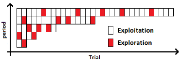
(a) Exemplary exploration-exploitation trade-off.

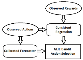
(b) Selection strategy flowchart (Algorithm 2).

Figure 1: Visualization of the proposed selection strategy.

Algorithm 2 Bandit Selection Strategy ($\chi$)

1:  Define an increasing sequence of integers, $T^{\prime}_{r}=2^{r}$ for $r=1,2,...$. Each member $T^{\prime}_{r}$ of this sequence denotes the length of period $r$, i.e. the number of trials included in it.

2:  Define a decreasing sequence of numbers, $Z_{r}=\frac{r}{2^{r}}$ for $r=1,2,...$.

3:  Set the period $r=1$ and select the exploration parameter $\gamma\ll 1$.

4:  repeat

5:     Select $\left\lceil T^{\prime}_{r}\cdot Z_{r}\right\rceil$ exploration trials belonging to $[1+\sum_{r}T^{\prime}_{r-1},\sum_{r}T^{\prime}_{r}]$ uniformly at random.

6:     for $t=s+\sum_{r}T^{\prime}_{r-1}$, $1\leq s<T^{\prime}_{r}$, do

7:        if $t$ is an exploring trial, then

8:           with probability $1-\gamma$, select an arm equally at random;with probability $\gamma$,1. receive the output of the forecaster (Algorithm 1),2. using this information, select the arm with the highest estimated expected reward.

9:        else

10:           Receive the input from the forecaster.

11:           Using this information, select the arm with the highest estimated expected reward.

12:        end if

13:        Play the selected arm and observe the reward.

14:        Observe the actions of other players and inform the forecaster (forecaster’s input).

15:        Re-estimate the mean reward function of the played arm.

16:     end for

17:     $r=r+1$.

18:  until convergence ($r$ is sufficiently large)

V-B Strong-Consistency and Convergence

The following results ensure the consistency and declare the convergence characteristics of the proposed selection strategy.

Lemma 1.

$T^{\prime}_{r}=2^{r}$ and $Z_{r}=\frac{r}{2^{r}}$ satisfy Assumption A3.

Proof:

The lemma can be easily verified by direct calculation using theorems concerning limits of infinite sequences. ∎

Lemma 2.

Consider a selection strategy $\kappa$ so that each player $k$ plays with actions based on $\delta_{d_{t}}$ ($m_{k,t}=\kappa(\delta_{d_{t}})$), where $\delta_{d_{t}}$ is the Dirac probability distribution on the true joint action profile of its opponents at time $t$. Let $\kappa^{\prime}$ be another strategy that is identical to $\kappa$, except that $P_{t}$ is used in the place of $\delta_{d_{t}}$ ($m_{k,t}=\kappa(P_{t})$), where $P_{t}$ is a probability distribution over all possible joint action profiles of opponents, produced by a calibrated forecaster. Then, $\lim_{T\to\infty}S_{\kappa,T}=1$ implies $\lim_{T\to\infty}S_{\kappa^{\prime},T}=1$, where $S_{\kappa,T}$ and $S_{\kappa^{\prime},T}$ are defined by (6).

Proof:

See Appendix VIII-A. ∎

Lemma 2 simply states that if a strategy is strongly consistent given true joint action profiles, then its consistency is preserved by using the calibrated forecast of the joint action profiles.

Lemma 3.

Asymptotically, the selection strategy $\chi$ samples each action $m\in\left\{1,...,M\right\}$ and also each joint action profile $\textbf{m}=(m_{1},...,m_{K})\in\bigotimes_{k=1}^{K}\left\{1,...,M\right\}$ infinitely often.

Proof:

See Appendix VIII-B. ∎

Theorem 3.

Under Assumptions A1, A2 and A3, the proposed selection strategy, $\chi$ (Algorithm 2), is strongly-consistent.

Proof:

See Appendix VIII-C. ∎

Theorem 4.

Consider a K-player MAB game where each player is provided with $M$ actions. Let $\mathfrak{C}$ denote the set of correlated equilbria, $\textbf{m}=(m_{1},..,m_{K})\in\bigotimes_{k=1}^{K}\left\{1,..,M\right\}$, and define the empirical joint frequencies of play as (9). If all players play according to selection strategy $\chi$, then the distance $\inf_{\pi\in\mathfrak{C}}\sum_{\textbf{m}}\left|\hat{\pi}_{T}(\textbf{m})-\pi(\textbf{m})\right|$ between the empirical joint distribution of plays and the set of correlated equilibria converges to $0$ almost surely as $T\to\infty$.

Proof:

See Appendix VIII-D. ∎

Remark 2.

In Section III-B, we mentioned that every player is interested in optimizing its performance in the sense of regret minimization, and no player intends to ruin the performance of others. Therefore players are rational and not malicious. By Remark 1 and Theorem 3, strategy $\chi$ yields vanishing regret; Thus the assumption that all players use this strategy is justified.

V-C Some Notes on Convergence Rate

As it is clear from Algorithm 2 (see also Figure 1(b)), for final convergence, the forecasting and regression procedures must converge to true joint action profile and true reward functions, respectively. In what follows, we discuss the impact of some variables, including number of actions ($M$) and users ($K$), as well as exploration parameter ($\gamma$), on the convergence rate of these procedures.

Theorem 5 ([26]).

For the calibrated forecaster given in Algorithm 1 we have

$$\limsup_{T\to\infty}\frac{T^{\frac{1}{D+1}}}{\sqrt{\ln(T)}}\sup_{B\in\mathfrak{B}}\left\|\frac{1}{T}\sum_{t=1}^{T}\mathbb{I}_{P_{t}\in B}(P_{t}-\delta_{d_{t}})\right\|_{1}\leq\Gamma_{D},$$ (13)

where $\mathfrak{B}$ is the Borel sigma-algebra of $\mathfrak{P}$ and the constant $\Gamma_{D}$ depends only on $D$.

From the algorithm we know that $D=M^{(K-1)}>1$. Figure 2(a) shows how the convergence rate scales with $D$ for $\Gamma_{D}=D$. As expected, convergence speed decreases for larger number of users $K$ and/or actions $M$, thereby larger $D$. Note that the effect of increasing $K$ on $D$ is more than that of $M$.

Now, consider the regression process, which is assumed to be non-parametric. Then the following holds.

Theorem 6 ([35]).

Consider a $p$-times differentiable unknown regression function $f$ and a $d$-dimensional measurement variable. Let $\hat{f}$ denote an estimator of $f$ based on a training sample of size $n$, and let $\left\|\hat{f}_{n}-f\right\|_{\infty}$ be the $L_{\infty}$ norm $\hat{f}_{n}-f$. Under appropriate regularity condition, the optimal rate of convergence for $\left\|\hat{f}_{n}-f\right\|_{\infty}$ to zero is $\left(\frac{\log(n)}{n}\right)^{\eta}$ where $\eta=\frac{p}{2p+d}$.

Based on Theorem 6, Algorithm 2 changes the convergence rate through changing the sampling rate. Assume that samples are gathered only at exploration trials. Let $R$ be the number of periods (game horizon). By the algorithm, each joint action profile is expected to be played $\frac{1-\gamma}{M^{K}}\sum_{r=1}^{R}r=\frac{1-\gamma}{M^{K}}\cdot\frac{R(R+1)}{2}$ times during $R$ periods (see also the proof of Lemma 3). Moreover, suppose that some fixed number of samples are required to estimate the reward of each joint action profile with some precision. Therefore, it is clear that increasing $M$ and/or $K$, as well as increasing $\gamma$, degrades the sampling rate and thereby the convergence speed, since larger game horizon is required for sufficient sampling. Let $B=\frac{1-\gamma}{M^{K}}<1$. Figure 2(b) shows how changes in $B$ impact the convergence speed of regression process.

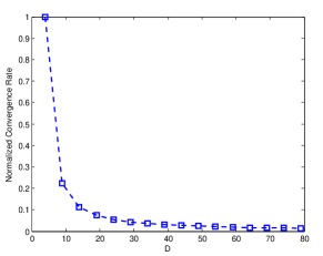
(a) Calibrated forecaster

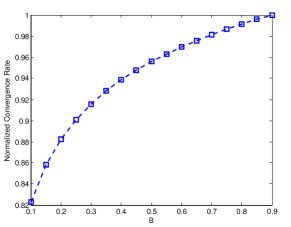
(b) Regression

Figure 2: Scaling convergence rate with variables and parameters ($M$, $K$ and $\gamma$), $D=M^{(K-1)}>1$ and $B=\frac{1-\gamma}{M^{K}}<1$.

VI Numerical Results

This section consists of two parts. First, we consider a simple model, and clarify how the algorithm works. Next we consider some larger network and the performance of the proposed approach is compared with some other approaches.

VI-A Part One

VI-A1 Network model

We consider an underlay D2D network consisting of two D2D users ($K=2$). We assume that there exist two primary channels ($M=2$), whose availability follows Bernoulli distribution with parameter $\frac{1}{2}$. We implement the following selection strategies.

• Statistical centralized strategy (SC): Given global statistical channel knowledge and by exhaustive search, a central controller assigns each D2D user some transmission channel so that the assignment corresponds to the most efficient pure strategy equilibrium point in the sense of maximum aggregate average throughput.

• Calibrated bandit strategy (CB): Provided with no prior information, D2D users simultaneously utilize the selection strategy $\chi$, described in Algorithm 2.

Since $M=2$, for each D2D user $k\in\left\{1,2\right\}$ we have $p_{k,1}+p_{k,2}=1$, where $p_{k,i}$ is the likelihood of D2D user $k$ to take action $i\in\left\{1,2\right\}$ by following the mixed strategy $(p_{k,1},p_{k,2})$. This implies that there exists only one degree of freedom in the $\epsilon$-grid of forecasters, i.e. for each player $k$ the probability distribution over all joint action profiles of opponents reduces here to the mixed strategy of the other player. We assume $N_{\epsilon}=40$. Therefore, the $\epsilon$-grid defines 40 possible mixed strategies (quantized vectors). The primal output of the forecaster of a player is a vector of weights including 40 elements, where each element denotes the likelihood of one of the quantized mixed strategies to be played by the other player. The final output of the forecaster is then a mixed strategy extracted from the set of quantized mixed strategies according to this distribution, as described in Algorithm 1.

VI-A2 Orthogonal Multiple Access

Assume that D2D users follow the orthogonal transmission scheme, described in Section II. Based on average channel gains, the joint rewards of players under possible joint action profiles are summarized in Table I. From this table, the channel selection game has a pure-strategy Nash equilibrium that yields the maximum aggregate reward for the two D2D users, and is achieved when D2D users 1 and 2 transmit in the first and second channels respectively (i.e. joint action (1,2)).

TABLE I: Joint reward table (orthogonal access)

channel	$1$	$2$
$1$	0.012,0.000	0.023,0.054
$2$	0.016,0.000	0.008,0.027

The average throughput achieved by each player is depicted in Figure 3. It can be seen that for sufficiently large game horizon (number of periods), the average throughput of our strategy converges to that of equilibrium.

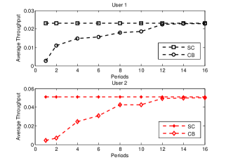
Figure 3: Average throughput of our approach versus that of centralized strategy (orthogonal access).

Actions of players are shown in Figure 4, at both early and final stages of the game, i.e. before and after the convergence, for 10 consecutive trials. By comparing this figure with the data given in Table I, it follows that the game converges to equilibrium, which is the joint action $(1,2)$. Moreover, the primal outputs of forecasters ($\psi$, see Algorithm 1) are shown in Figure 5(a), for some trial before convergence. In this figure, outputs are almost uniformly distributed, meaning that all quantized mixed strategies are almost equally likely to occur. This result is in agreement with Figure 4, where selected channels before convergence do not follow any specific pattern. On the other hand, outputs of forecasters at some trial after convergence are depicted in Figure 5(b). In this figure, Forecaster 1 assigns higher weights to quantized mixed strategies with $p_{2}>p_{1}$, while Forecaster 2 emphasizes the strategies with $p_{1}>p_{2}$. This means that first and second players are excepted to select channels 1 and 2, respectively, by their opponents. These predictions are again approved by Figure 4, where first and second D2D users finally settle at first and second channels, respectively.

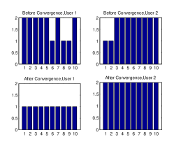
Figure 4: Selected actions before and after convergence (orthogonal access).

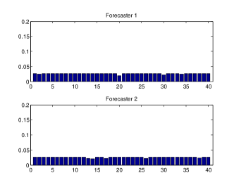
(a) Before convergence.

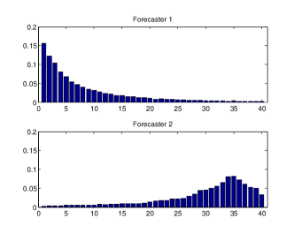
(b) After convergence.

Figure 5: Forecasters’ outputs (orthogonal access).

VI-A3 Non-orthogonal Multiple Access

As described in Section II, in case of non-orthogonal multiple access, conflicting D2D users transmit simultaneously, which might result in interference. In this scenario, players decide whether to solve the conflict by diverting to different channels, or to transmit in a common channel. In order to clarify this, we perform two experiments. For the first and second experiments, joint rewards are given by Table II(a) and Table II(b), respectively.

channel	$1$	$2$
$1$	0.024,0.040	0.024,0.021
$2$	0.075,0.042	0.063,0.021

(a) Case 1

channel	$1$	$2$
$1$	0.024,0.001	0.024,0.021
$2$	0.075,0.000	0.063,0.021

(b) Case 2

TABLE II: Joint reward table (non-orthogonal access)

From these tables, the most efficient pure-strategy equilibrium points for the first and second games are joint actions $(2,1)$ and $(2,2)$ respectively. This means that in the first case, it is beneficial for players transmit in different channels, while in the second case, D2D users achieve higher gains if both transmit through the second channel.

The achieved throughput by players are shown in Figures 6(a) and 6(b), respectively for the two experiments. Moreover, Figures 7(a) and 7(b) show the actions of players for first and second experiments. Figures 8(a) and 8(b), at a single trial after convergence (the outputs of forecasters before convergence are similar to Figure 5(a)). Descriptions are similar to the orthogonal case, and are omitted for space considerations.

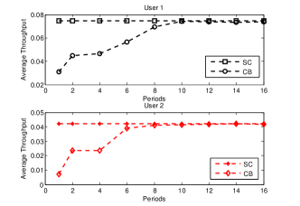
(a) Case 1

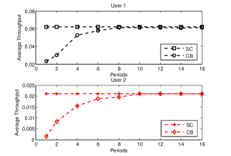
(b) Case 2

Figure 6: Average throughput of our approach versus that of equilibrium (non-orthogonal access).

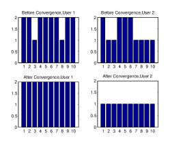
(a) Case 1

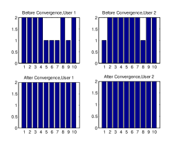
(b) Case 2

Figure 7: Selected actions before and after convergence (non-orthogonal access).

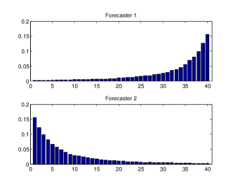
(a) Case 1

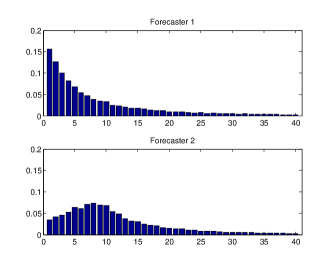
(b) Case 2

Figure 8: Forecasters’ outputs after convergence (non-orthogonal access).

VI-B Part Two

Consider a D2D network with 4 users and 4 primary channels. The performance metric is the aggregate average throughput of users, and the following approaches are compared.

• Statistical centralized strategy (SC) : This approach is described in Section VI-A1.

• Calibrated bandit strategy (CB): This is our proposed selection strategy (Algorithm 2).

• No collision bandit strategy (NCB): Following [21], stochastic multi-armed bandit game is played, where in case of collision, no reward is assigned to colliding users.

• $\epsilon$-greedy Q-learning strategy (GQL): Let $0<\epsilon<1$. Each player assigns some Q-value to each action-state pair. At each trial, every player selects the action that has yield the largest Q-value so far with probability $1-\epsilon$, and an action uniformly at random with probability $\epsilon$. After playing, the Q-value of the selected action and observed state is updated [36]. Note that no forecasting is performed, thus the best-response dynamics cannot be applied.

• Availability-based Strategy (AB) : As described in [16], this model ignores the role of channel qualities in the reward achieved by players. More precisely, the learning approach includes only the availability of channels and the number of users willing to transmit through each channel.

• Uniformly Random Strategy (UR): At each trial, an action is selected uniformly at random.

Results are depicted in Figure 9, and discussed briefly in the following.

• CB requires some time to converge to the average throughput achieved by SC. It yields no overhead, however, since unlike SC, D2D users are not required to establish direct contact with the BS. Computational effort is also much less than that of SC.

• The performance of GQL algorithm is inferior to the performance of CB. This is mainly due to the absence of forecasting and best-response dynamics. Note that in addition to aggregate performance loss, simple $\epsilon$-greedy algorithms without forecasting do not guarantee that the game converge to an equilibrium.

• The main reason that NCB performs poor is that the collision is not allowed. In such condition, even if it is better for D2D users to collide (similar to the result of Section VI-A3, case 2), the approach makes them to choose different channels.

• Similar to GQL, AB does not exhibit good performance in comparison to CB. The reason is obvious. While CB takes channel quality and availability into account, AB is only based on channel availability. Intuitively, the performance of AB is in direct relation with channel qualities. More precsiely, for channels with similar and/or large gains, the harmful effect of ignoring channel qualities is alleviated. The advantagemof this approach is its zero overhead.

• Uniform random strategy yields the worst performance. However, it is also the simplest approach, with respect to information flow and computational effort.

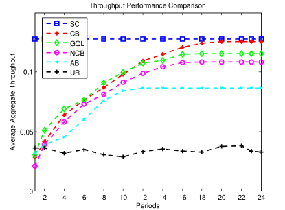
Figure 9: Throughput performance comparison.

VII Conclusion and Remarks

We studied a channel selection problem in an underlay distributed D2D communication system. In this model, spectrum vacancies of the cellular network are utilized by D2D users, thereby boosting the spectrum efficiency and improving local services, with no adverse effect on cellular users. Each D2D user aims at maximizing its performance given no prior information, and achieving an equilibrium is beneficial for all users. We showed that the channel selection problem boils down to a multi-player multi-armed bandit game with side information, and we proposed an approach to solve this game by combining no-regret bandit learning with calibrated forecasting. Analytically, we established that the proposed strategy is strongly-consistent; that is, for each D2D user, the average accumulated reward in the long run is equal to that based on the best fixed strategy in te sense of aggregate average reward. Moreover, we proved that the proposed approach converges to an equilibrium in some sense. Numerical analysis verified analytical results.

VIII Appendix

VIII-A Proof of Lemma 2

We follow a root suggested in [32]. Suppose that $\lim_{T\to\infty}S_{\kappa,T}=1$ holds. In order to prove $\lim_{T\to\infty}S_{\kappa^{\prime},T}=1$, it is sufficient to show that after some finite time, the actions taken by the player based on $\mathbf{P}_{t}$ are equal to those based on $\delta_{d_{t}}$. By (7), we know that, with probability 1, there exists an $\nu>0$ so that after a time point $\theta<\infty$,

$$\left|\mathbf{P}_{t}-\delta_{d_{t}}\right|<\nu$$ (14)

holds for all $t>\theta$ (see also Theorem 2). At the same time, according to our system model and by Assumption A1, the reward functions are bounded, and the action space and memory are finite. This implies that if (14) holds, then the actions of the player evolve as if it were aware of the true joint action profile of its opponents. Hence the lemma follows.

VIII-B Proof of Lemma 3

From Algorithm 2, at each period $r$, $\left\lceil T^{\prime}_{r}\cdot Z_{r}\right\rceil$ trials are selected for exploration by each player. At each one of these trials, with probability $1-\gamma$, an arm $m$ is selected equally at random. Since these processes are independent, the probability that arm $m$ is pulled at some exploration trial yields $\frac{1-\gamma}{M}$. Now, let $\left\{W_{t}^{(m)}\right\}_{t=1}^{T}$ be a sequence of random variables, where $W_{t}^{(m)}=1$ if arm $m$ is played at time $t$, and $W_{t}^{(m)}=0$ otherwise, and the outcomes $W_{t}^{(m)}$ are independent over time. In the worst-case, arm $m$ never becomes the best-response, and hence its chance of being played is limited to exploration trials. As a result, $\textup{Pr}\left[W_{t}^{(m)}=1\right]=\frac{1-\gamma}{M}$, and the sum of probabilities for the event $W_{t}^{(m)}=1$ yields $\sum_{t=1}^{T}\textup{Pr}\left[W_{t}=1\right]=\frac{1-\gamma}{M}\sum_{r=1}^{R}\left\lceil T^{\prime}_{r}\cdot Z_{r}\right\rceil$. By using Assumption A3 and Lemma 1, we conclude that $\lim_{T\to\infty}\sum_{t=1}^{T}\textup{Pr}\left[W_{t}=1\right]\to\infty$. Thus, by the second Borel-Cantelli lemma ([32], [37]), it follows that the probability of arm $m$ being pulled infinitely often equals 1. On the other hand, players select their actions independently. As such, the probability of playing each joint action profile is given by $\frac{1-\gamma}{M^{K}}$. By the same argumentation, each joint action profile is also played infinitely often. Hence, the Lemma is proved.

VIII-C Proof of Theorem 3

Since the proof is identical for all players, we prove the strong-consistency for some player $k$, and hence omit the player’s subscript, $k$, for brevity. It should be mentioned that the proof is inspired by [29], where the authors showed the consistency of an allocation rule for single-player contextual bandit games, which, similar to our algorithm, follows the GLIE rule.

In the following, we consider a selection strategy $\chi^{\prime}$, which is identical to $\chi$, except that at each time $t$ and before taking any action, the player is informed about the true joint action profile of other $K-1$ players, that is $k^{-}_{t}$. We prove that $\chi^{\prime}$ is strongly-consistent. Therefore, from Lemma 2 it follows that $\chi$ is strongly-consistent, as well.

In what follows, $m_{t}$ is used to denote the selected arm at time $t$, while $\hat{m}_{t}$ stands for the arm with the highest estimated expected reward at time $t$. That is, at time $t$ we have $\hat{f}_{\hat{m}_{t}}(k^{-}_{t})\coloneqq\max_{m\in\left\{1,..,M\right\}}\hat{f}_{m}(k^{-}_{t})$. Moreover, $m^{*}_{t}$ denotes the arm with the highest true expected reward at time $t$ so that $f_{m^{*}_{t}}(k^{-}_{t})\coloneqq\max_{m\in\left\{1,..,M\right\}}f_{m}(k^{-}_{t})$. Ties are broken using some deterministic rule.

From Definition 1, $S_{\chi^{\prime},T}$ is upper bounded by 1. Therefore, it is sufficient to prove a lower bound on $S_{\chi^{\prime},T}$ that converges to $1$ as $T\to\infty$. To this end, we rewrite $S_{\chi^{\prime},T}$ as [29]

$$S_{\chi^{\prime},T}=\frac{\sum_{t=1}^{T}f_{\hat{m}_{t}}(k_{t}^{-})}{\sum_{t=1}^{T}f_{m_{t}^{*}}(k_{t}^{-})}+\frac{\sum_{t=1}^{T}(f_{m_{t}}(k_{t}^{-})-f_{\hat{m}_{t}}(k_{t}^{-}))}{\sum_{t=1}^{T}f_{m_{t}^{*}}(k_{t}^{-})}\leq 1.$$ (15)

By Assumption A1, it follows from (15) that

$$S_{\chi^{\prime},T}\geq\frac{\sum_{t=1}^{T}f_{\hat{m}_{t}}(k_{t}^{-})}{\sum_{t=1}^{T}f_{m_{t}^{*}}(k_{t}^{-})}-\frac{\frac{1}{T}\sum_{t=1}^{T}B\mathbb{I}_{\left\{m_{t}\neq\hat{m}_{t}\right\}}}{\frac{1}{T}\sum_{t=1}^{T}f_{m_{t}^{*}}(k_{t}^{-})}.$$ (16)

The remainder of the proof consists of two parts. In the first part we show that

$$\frac{\frac{1}{T}\sum_{t=1}^{T}B\mathbb{I}_{\left\{m_{t}\neq\hat{m}_{t}\right\}}}{\frac{1}{T}\sum_{t=1}^{T}f_{m_{t}^{*}}(k_{t}^{-})}\overset{\textup{a.s.}}{\rightarrow}0,~{}\textup{as}~{}~{}T\rightarrow\infty,$$ (17)

while the second part deals with

$$\frac{\sum_{t=1}^{T}f_{\hat{m}_{t}}(k_{t}^{-})}{\sum_{t=1}^{T}f_{m_{t}^{*}}(k_{t}^{-})}\overset{\textup{a.s.}}{\rightarrow}1,~{}\textup{as}~{}~{}T\rightarrow\infty.$$ (18)

Combining (17) and (18) with (16) and $S_{\chi^{\prime},T}\leq 1$ proves the strong consistency.
(i) By Assumption A1, $\sum_{t=1}^{T}f_{m_{t}^{*}}(k_{t}^{-})$ is positive. As a result, $\frac{1}{T}\sum_{t=1}^{T}f_{m_{t}^{*}}(k_{t}^{-})$ converges to $\textup{E}_{t}\left\{f_{m_{t}^{*}}(k_{t}^{-})\right\}>0$ almost surely. Hence, it suffices to show that $\frac{1}{T}\sum_{t=1}^{T}B\mathbb{I}_{\left\{m_{t}\neq\hat{m}_{t}\right\}}\rightarrow 0$, almost surely. To show this, we consider the worst-case; that is, we assume that in all exploration trials, inferior arms are selected (i.e. the best-response is never selected by chance). Therefore

$$\lim_{T\to\infty}\frac{1}{T}\sum_{t=1}^{T}B\mathbb{I}_{\left\{m_{t}\neq\hat{m}_{t}\right\}}=\lim_{R\to\infty}\frac{\sum_{r=1}^{R}\left\lceil T^{\prime}_{r}Z_{r}\right\rceil}{\sum_{r=1}^{R}T^{\prime}_{r}}=0,$$ (19)

where the second equality follows from Assumption A3 and Lemma 1. This proves (17).
(ii) First, we note that (18) is equivalent to [29]

$$\frac{\sum_{t=1}^{T}(f_{\hat{m}_{t}}(k_{t}^{-})-f_{m_{t}^{*}}(k_{t}^{-}))}{\sum_{t=1}^{T}f_{m_{t}^{*}}(k_{t}^{-})}\overset{\textup{a.s.}}{\rightarrow}0,~{}\textup{as}~{}~{}T\rightarrow\infty.$$ (20)

Moreover, by (15), (16) and (17), we conclude that

$$\frac{\sum_{t=1}^{T}(f_{\hat{m}_{t}}(k_{t}^{-})-f_{m_{t}^{*}}(k_{t}^{-}))}{\sum_{t=1}^{T}f_{m_{t}^{*}}(k_{t}^{-})}\leq 0.$$ (21)

Clearly,

$$f_{\hat{m}_{t}}(k_{t}^{-})-f_{m_{t}^{*}}(k_{t}^{-}) =f_{\hat{m}_{t}}(k_{t}^{-})-\hat{f}_{\hat{m}_{t},t-1}(k_{t}^{-})+\hat{f}_{\hat{m}_{t},t-1}(k_{t}^{-})$$ (22)

$$-\hat{f}_{{m_{t}^{*}},t-1}(k_{t}^{-})+\hat{f}_{m_{t}^{*},t-1}(k_{t}^{-})-f_{m_{t}^{*}}(k_{t}^{-}).$$

On the other hand, for every trial $t$, $\hat{f}_{\hat{m}_{t},t-1}(k_{t}^{-})\geq\hat{f}_{m^{*}_{t},t-1}(k_{t}^{-})$ holds. Hence we can write [29]

$$f_{\hat{m}_{t}}(k_{t}^{-}) -f_{m_{t}^{*}}(k_{t}^{-})$$ (23)

$$\geq f_{\hat{m}_{t}} (k_{t}^{-})-\hat{f}_{\hat{m}_{t},t-1}(k_{t}^{-})-f_{{m_{t}^{*}}}(k_{t}^{-})+\hat{f}_{{m_{t}^{*}},t-1}(k_{t}^{-})$$

$$\geq-2{} \sup_{1\leq m\leq M}\left\|\hat{f}_{m,t-1}(k_{t}^{-})-f_{m}(k_{t}^{-})\right\|_{\infty}.$$

This yields

$$\frac{\sum_{t=1}^{T}(f_{\hat{m}_{t}}(k_{t}^{-})-f_{m_{t}^{*}}(k_{t}^{-}))}{\sum_{t=1}^{T}f_{m_{t}^{*}}(k_{t}^{-})}$$ (24)

$$\geq\frac{\frac{-2}{T}\sum_{t=1}^{T}\sup_{1\leq m\leq M}\left\|\hat{f}_{m,t-1}(k_{t}^{-})-f_{m}(k_{t}^{-})\right\|_{\infty}}{\frac{1}{T}\sum_{t=1}^{T}f_{m_{t}^{*}}(k_{t}^{-})}.$$

For brevity, let us rewrite (24) in a shorter form as $a\geq b$. By Assumption A2, $\|\hat{f}_{m,T}(k^{-})-f_{m}(k^{-})\|_{\infty}\to 0$ as $T\to\infty$. However, in order to use this assumption, we need to ensure that not only each arm, but also each joint action profile is played infinitely many times, as $T\to\infty$. This is established in Lemma 3. Therefore, the right-hand side of (24) converges to zero, i.e. $b\to 0$ and hence $a\geq 0$. On the other hand, by (21), the left-hand side is upper-bounded by zero, that is $a\leq 0$. As a result, (20) follows, which completes the second part of the proof.

VIII-D Proof of Theorem 4

Consider a K-player MAB game, as described in Section III-A. By Theorem 1, if each player plays by best responding to a calibrated forecast of the joint action profile of opponents, then

$$\inf_{\pi\in\mathfrak{C}}\sum_{\textbf{m}}\left|\hat{\pi}_{T}(\textbf{m})-\pi(\textbf{m})\right|\to 0,$$ (25)

as $T\to\infty$. We refer to this selection strategy as $\chi^{\prime}$. In order to prove the Theorem, we show that our strategy $\chi$, in which the true expected rewards of joint action profiles are not known and are gradually learned by exploration, exhibits the same convergence characteristics as $\chi^{\prime}$.

First, we re-arrange the K-player MAB game to a two-agent game where the first agent is any player $k$ and the second agent is the set of its opponents, i.e. the set of $K-1$ players. For this game, any joint action profile of the two agents can be written as $(m,\textbf{m}^{-})$, where $m\in\left\{1,...,M\right\}$ and $\textbf{m}^{-}\in\bigotimes_{k=1}^{K-1}\left\{1,...,M\right\}$. Let $\hat{\pi}_{T}(m,\textbf{m}^{-})$ denote the fraction of time until $T$ in which some joint action $(m,\textbf{m}^{-})$ is played. According to selection strategy $\chi$, $\hat{\pi}_{T}(m,\textbf{m}^{-})$ can be written as

$$\hat{\pi}_{T}(m,\textbf{m}^{-})=\hat{\pi}_{T,r}(m,\textbf{m}^{-})+\hat{\pi}_{T,i}(m,\textbf{m}^{-}),$$ (26)

where $\hat{\pi}_{T,r}(m,\textbf{m}^{-})$ and $\hat{\pi}_{T,i}(m,\textbf{m}^{-})$ denote the fractions of time in which $(m,\textbf{m}^{-})$ is played by exploration (i.e. by chance), and by exploitation (i.e. according to the best response rule given by (10)), respectively. According to Algorithm 2, the total number of exploration trials is given by $\sum_{r=1}^{R}\left\lceil T^{\prime}_{r}Z_{r}\right\rceil$. Moreover, by Assumption A3, we know

$$\lim_{R\to\infty}\frac{\sum_{r=1}^{R}\left\lceil T^{\prime}_{r}Z_{r}\right\rceil}{\sum_{r=1}^{R}T^{\prime}_{r}}=0.$$ (27)

This implies that

$$\hat{\pi}_{T,r}(m,\textbf{m}^{-})=0,$$ (28)

for $T\to\infty$. Therefore, in the limit, $\hat{\pi}_{T,r}(m,\textbf{m}^{-})$ can be neglected when calculating the empirical frequencies of plays, and

$$\hat{\pi}_{T}(m,\textbf{m}^{-})=\hat{\pi}_{T,i}(m,\textbf{m}^{-})$$ (29)

holds asymptotically.
In order to complete the proof, it is sufficient to show that after some finite time, the actions taken by the player based on $\hat{f}_{m,k,t}$ are equal to those based on $f_{m,k}$. By Assumption A1, we know that, with probability 1, there exists an $\nu>0$ so that for every $m\in\left\{1,...,M\right\}$ and after a time point $\theta<\infty$,

$$\|\hat{f}_{m,k}(k^{-})-f_{m,k}(k^{-})\|<\nu,$$ (30)

holds for all $t>\theta$. At the same time, according to our system model and by Assumption A1, the reward functions are bounded, and the action space and memory are finite. This implies that if (30) holds, then the actions of the player evolve as if it were aware of the true expected reward of each joint action profile, which completes the proof.

References

- [1] G. Fodor, E. Dahlman, G. Mildh, S. Parkvall, N. Reider, G. Miklos, and Z. Turanyi, “Design aspects of network assisted device-to-device communications,” IEEE Communications Magazine, vol. 50, no. 3, pp. 170–177, 2012.
- [2] L. Lei, Z. Zhong, C. Lin, and X. Shen, “Operator controlled device-to-device communications in LTE-advanced networks,” IEEE Wireless Communications, vol. 19, no. 3, pp. 96–104, 2012.
- [3] J. Feng, S. Saoudi, and T. Derham, “Centralized scheduling of in-band device-to-device communication underlaying cellular networks,” in International Symposium on Wireless Personal Multimedia Communications, 2013, pp. 1–5.
- [4] T. Han, R. Yin, Y. Xu, and G. Yu, “Uplink channel reusing selection optimization for device-to-device communication underlaying cellular networks,” in IEEE International Symposium on Personal, Indoor and Mobile Radio Communications, 2012, pp. 559–564.
- [5] H. Wang and X. Chu, “Distance-constrained resource-sharing criteria for device-to-device communications underlaying cellular networks,” Electronics Letters, vol. 48, no. 9, pp. 528–530, 2012.
- [6] C. Xu, L. Song, Z. Han, Q. Zhao, X. Wang, and B. Jiao, “Interference-aware resource allocation for device-to-device communications as an underlay using sequential second price auction,” in IEEE International Conference on Communications, 2012, pp. 445–449.
- [7] C. Xu, L. Song, Z. Han, Q. Zhao, X. Wang, X. Cheng, and B. Jiao, “Efficiency resource allocation for device-to-device underlay communication systems: A reverse iterative combinatorial auction based approach,” IEEE Journal on Selected Areas in Communications, vol. 31, no. 9, pp. 348–358, 2013.
- [8] F. Wang, L. Song, Z. Han, Q. Zhao, and X. Wang, “Joint scheduling and resource allocation for device-to-device underlay communication,” in IEEE Wireless Communications and Networking Conference, 2013, pp. 134–139.
- [9] E. Yaacoub and O. Kubbar, “Energy-efficient device-to-device communications in LTE public safety networks,” in IEEE Globecom Workshops, 2012, pp. 391–395.
- [10] S. Maghsudi and S. Stanczak, “A hybrid centralized-decentralized resource allocation scheme for two-hop transmission,” in 8th International Symposium on Wireless Communication Systems, 2011, pp. 96–100.
- [11] Z. Khan, S. Glisic, L.A. DaSilva, and J. Lehtoma ki, “Modeling the dynamics of coalition formation games for cooperative spectrum sharing in an interference channel,” IEEE Transactions on Computational Intelligence and AI in Games, vol. 3, no. 1, pp. 17–30, 2011.
- [12] S. Sodagari, A. Attar, and S.G. Bilen, “On a truthful mechanism for expiring spectrum sharing in cognitive radio networks,” IEEE Journal on Selected Areas in Communications, vol. 29, no. 4, pp. 856–865, 2011.
- [13] M. Guo, Y. Liu, and J. Malec, “A new Q-learning algorithm based on the metropolis criterion,” IEEE Transactions on Systems, Man, and Cybernetics, Part B: Cybernetics, vol. 34, no. 5, pp. 2140–2143, 2004.
- [14] X. Fang, D. Yang, and G. Xue, “Taming wheel of fortune in the air: An algorithmic framework for channel selection strategy in cognitive radio networks,” IEEE Transactions on Vehicular Technology, vol. 62, no. 2, pp. 783–796, 2013.
- [15] Y. Song, Y. Fang, and Y. Zhang, “Stochastic channel selection in cognitive radio networks,” in IEEE Global Telecommunications Conference, 2007, pp. 4878–4882.
- [16] Y. Xu, J. Wang, Q. Wu, A. Anpalagan, and Y.D. Yao, “Opportunistic spectrum access in unknown dynamic environment: A game-theoretic stochastic learning solution,” IEEE Transactions on Wireless Communications, 2012.
- [17] Y. Xu, Q. Wu, L. Shen, J. Wang, and A. Anpalagan, “Opportunistic spectrum access with spatial reuse: Graphical game and uncoupled learning solutions,” IEEE Transactions on Wireless Communications, 2013.
- [18] Y. Xu, Q. Wu, J. Wang, L. Shen, and A. Anpalagan, “Opportunistic spectrum access using partially overlapping channels: Graphical game and uncoupled learning,” IEEE Transactions on Communications, 2013.
- [19] W. Xu, L. Liang, H. Zhang, S. Jin, J.C.F. Li, and M. Lei, “Performance enhanced transmission in device-to-device communications: Beamforming or interference cancellation?,” in IEEE Global Communications Conference, 2012, pp. 4296–4301.
- [20] N. D. Kalathil, Nayyar, and R. Jain, “Multi-player multi-armed bandits: Decentralized learning with iid rewards,” in Annual Allerton Conference on Communication, Control, and Computing, Oct 2012, pp. 853–860.
- [21] D. Kalathil, N. Nayyar, and R. Jain, “Decentralized learning for multi-player multi-armed bandits,” in IEEE Annual Conference on Decision and Control, Dec 2012, pp. 3960–3965.
- [22] D. Kalathil, N. Nayyar, and R. Jain, “Decentralized learning for multiplayer multiarmed bandits,” IEEE Transactions on Information Theory, vol. 60, no. 4, pp. 2331–2345, April 2014.
- [23] K. Liu, Q. Zhao, and B. Krishnamachari, “Decentralized multi-armed bandit with imperfect observations,” in Annual Allerton Conference on Communication, Control, and Computing, Sept 2010, pp. 1669–1674.
- [24] K. Liu and Q. Zhao, “Distributed learning in multi-armed bandit with multiple players,” IEEE Transactions on Signal Processing, vol. 58, no. 11, pp. 5667–5681, Nov 2010.
- [25] H. Liu, K. Liu, and Q. Zhao, “Learning in a changing world: Restless multiarmed bandit with unknown dynamics,” IEEE Transactions on Information Theory, vol. 59, no. 3, pp. 1902–1916, March 2013.
- [26] S. Mannor and G. Stoltz, “A geometric proof of calibration,” Mathematics of Operations Research, vol. 35, no. 4, pp. 721–727, 2010.
- [27] S.M. Kakade and D.P. Foster, “Deterministic calibration and Nash equilibrium,” Elsevier Journal of Computer and System Sciences, vol. 74, pp. 115–130, 2008.
- [28] D.P. Foster and R. Vohra, “Calibrated learning and correlated equilibrium,” Games and Economic Behavior, vol. 21, pp. 40–55, 1997.
- [29] Y. Yang and D. Zhu, “Randomized allocation with nonparametric estimation for a multi-armed bandit problem with covariates,” The Annals of Statistics, vol. 30, no. 1, pp. 100–121, 2002.
- [30] N. Cesa-Bianchi and G. Lugosi, Prediction, Learning, and Games, Cambridge University Press, 2006.
- [31] S. Singh, T. Jaakkola, M.L. Littman, and C. Szepesvari, “Convergence results for single-step on-policy reinforcement-learning algorithms,” Machine Learning, vol. 38, no. 3, pp. 287–308, 2000.
- [32] A.C. Chapman, D.S. Leslie, A. Rogers, and N.R. Jennings, “Convergent learning algorithms for unknown reward games,” SIAM Journal on Control and Optimization, vol. 51, no. 4, pp. 3154–3180, 2013.
- [33] Q. Zhao, L. Tong, A. Swami, and Y. Chen, “Decentralized cognitive MAC for opportunistic spectrum access in ad hoc networks: A POMDP framework,” IEEE Journal on Selected Areas in Communications, vol. 25, no. 3, pp. 589–600, April 2007.
- [34] Y. Freund and R.E. Schapire, “Adaptive game playing using multiplicative weights,” Games and Economic Behavior, vol. 29, no. 1, pp. 79–103, 1999.
- [35] C.J. Stone, “Optimal global rates of convergence for nonparametric regression,” The Annals of Statistics, vol. 10, no. 4, pp. 1040–1053, 1982.
- [36] M. Bennis, S. Guruacharya, and D. Niyato, “Distributed learning strategies for interference mitigation in femtocell networks,” in IEEE Global Telecommunications Conference, Dec 2011, pp. 1–5.
- [37] W. Feller, An Introduction to Probability Theory and Its Applications, vol. 1, Wiley, 1968.