Superintegrable Lissajous systems on the sphere

Abstract

A kind of systems on the sphere, whose trajectories are similar to the Lissajous curves, are studied by means of one example. The symmetries are constructed following a unified and straightforward procedure for both the quantum and the classical versions of the model. In the quantum case it is stressed how the symmetries give the degeneracy of each energy level. In the classical case it is shown how the constants of motion supply the orbits, the motion and the frequencies in a natural way.

1 Introduction

The well known Lissajous curves in two dimensions (2D) correspond to the motion of a system that can be described by two cartesian coordinates, where each coordinate is harmonic in time and the ratio of both frequencies is a rational number. Such curves are closed in a rectangle and depend on the phase difference at the initial time. In a similar way, we want to extend this point of view to systems on the sphere where the motion is obtained in terms of the spherical coordinates $\varphi(t)$ and $\theta(t)$. In this case, the motion in each coordinate will be periodic but not harmonic, and their trajectories closed curves inscribed in a ‘spherical rectangle’, $\varphi_{1}\leq\varphi\leq\varphi_{2}$, $\theta_{1}\leq\theta\leq\theta_{2}$, when the proportion of the two periods is a rational number.

The type of systems leading to Lissajous type trajectories include the TTW [1, 2] and other similar systems [3, 4, 5, 6, 7, 8, 9]. They are superintegrable and the search of their symmetries has been the subject of a considerable number of recent contributions. In this work, by means of one example, we want to stress the features of such systems defined on the sphere leading to Lissajous like curves. In particular it will be shown how the trajectories are determined and how the period of the motion in each coordinate can be computed by means of pure algebraic methods. We will adopt a simple procedure presented in [10] in order to deal with the symmetries and constants of motion.

Let us emphasize the main novelties of our approach: (i) The method to find the symmetries for both the quantum and the classical versions of these systems follow the same pattern. In previous references, quite different procedures were applied in order to obtain classical or quantum symmetries, as a consequence, the origin of the close relationship of classical and quantum algebraic relations was hidden from the very beginning. (ii) Our way relies on simple arguments based on the factorization properties of one–dimensional systems [11, 12, 13]. This method, well known in quantum mechanics, is extended to classical systems. For instance, we can define in a straightforward way ‘ladder functions’ and ‘shift functions’ whose counterpart operators are familiar in quantum mechanics. (iii) As we will see later, the classical version of our 2D system is maximally superintegrable, so that we can find three independent constants of motion (with two of them in involution). These constants will characterize the orbits. However, one additional constant of motion, depending explicitly on time, is obtained from some ‘ladder functions’. This additional constant of motion will determine the motion of the system along each orbit.

In summary, we have a kind of ‘complete superintegrability’ where the number of independent integrals of motion is ‘$(2n-1)+1=2n$’ characterizing completely the motion (not only the trajectory). The symmetries or constants of motion in this paper include square roots that, in the case of operators, can only be defined when they act on eigenfunctions. Hence, the symmetries are not polynomial in the momentum operators. However they can be translated into polynomial symmetries in a simple way, as it will be shown in a forthcoming work [14].

The paper is organized as follows. Section 2 is devoted to the quantum version of our example. This system can be considered as a composition of two one–dimensional trigonometric Pöschl–Teller (PT) potentials. Therefore, the well known factorization properties of the PT component systems can be straightforwardly applied in order to get the symmetries of the composed system. It will be shown how these symmetries explain the degeneracy of each energy level. Section 3 will be dedicated to the classical system whose constants of motion are found by implementing the methods used previously in the quantum case. These symmetries will determine the trajectories and their properties as Lissajous curves. Section 4 will be concerned with the motion of the system. In this case, the motion can also be obtained in an algebraic way by means of the aforementioned additional constant of motion depending explicitly on time. In particular, the frequency takes part of the algebraic properties through Poisson brackets. Some comments and remarks in Section 5 on the special character of Lissajous systems will end the paper.

2 The quantum system

The Hamiltonian operator that we will consider in this paper belongs to a type of Smorodinsky–Winternitz systems on the sphere [15, 16]. It depends on a real coupling parameter, $k$, and has the following form (the units $2m=1$ and $\hbar=1$ have been chosen to simplify the formulas):

$$\hat{H}=-\partial^{2}_{\theta}-\cot{\theta}\partial_{\theta}-\frac{1}{\sin^{2}{\theta}}\partial^{2}_{\varphi}-\frac{k^{2}}{\sin^{2}{\theta}}\left(\frac{1/4-\alpha^{2}}{\cos^{2}{k\,\varphi}}+\frac{1/4-\beta^{2}}{\sin^{2}{k\,\varphi}}\right)$$ (1)

where $0<\theta<\pi$ and $0<\varphi<\pi/2k$. The first three terms correspond to the Laplacian in spherical coordinates, the last term is for the potential. It should be remarked that $k$ must satisfy $k\geq 1/4$, so that the system be well defined in a region of the sphere.

First of all, the change of variable ${k\,\varphi}=\phi$ will be performed, so that henceforth we will work with the following Hamiltonian [10]

$$\hat{H}=-\partial^{2}_{\theta}-\cot{\theta}\partial_{\theta}+\frac{k^{2}}{\sin^{2}{\theta}}\left(-\partial^{2}_{\phi}+\frac{\alpha^{2}-1/4}{\cos^{2}{\phi}}+\frac{\beta^{2}-1/4}{\sin^{2}{\phi}}\right)\,,$$ (2)

where now, the angle $\phi$ will range in the interval $(0,\pi/2)$. The corresponding eigenvalue equation is

$$\hat{H}\,\Psi(\theta,\phi)=E\,\Psi(\theta,\phi)\,.$$ (3)

It is clear that the Hamiltonian (2) is separated in the spherical coordinates $(\theta,\phi)$, so we will look for separable solutions, $\Psi(\theta,\phi)=\Theta(\theta)\,\Phi(\phi)$. This type of solutions are characterized by

$$\hat{H}^{M}_{\theta}\,\Theta(\theta)=E_{\theta}\,\Theta(\theta),\quad\hat{H}_{\phi}\,\Phi(\phi)=E_{\phi}\,\Phi(\phi),$$ (4)

where the one–dimensional Hamiltonians are

$$\hat{H}^{M}_{\theta}=-\partial^{2}_{\theta}-\cot{\theta}\partial_{\theta}+\frac{M^{2}}{\sin^{2}{\theta}}\,,$$ (5)

which has a form equivalent to a one–parameter trigonometric PT Hamiltonian, and

$$\hat{H}_{\phi}=-\partial^{2}_{\phi}+\frac{\alpha^{2}-1/4}{\cos^{2}{\phi}}+\frac{\beta^{2}-1/4}{\sin^{2}{\phi}}$$ (6)

which is a two–parameter trigonometric PT potential. The following notation has been introduced

$$E_{\theta}:=E\,,\qquad E_{\phi}:=\epsilon^{2}\,,\qquad M^{2}:=k^{2}E_{\phi}=k^{2}\epsilon^{2}\,.$$ (7)

The case $\beta=\pm 1/2$ (or $\alpha=\pm 1/2$) in (6) corresponds to the one–parameter trigonometric PT potential (in this case, $\phi\in(-\pi/2,\pi/2)$ and $k\geq 1/2$).

In order to get the symmetries of $\hat{H}$, we will deal separately with each of these two one–dimensional problems by means of factorizations [12]. We will find ladder (lowering and raising) operators for $\hat{H}_{\phi}$ and shift operators for $\hat{H}_{\theta}$. As we will see later on, the ladder operators will act on the coefficient $k\epsilon$ of the Hamiltonian (5) for the two–parameter PT potential in the form (for the one–parameter PT potential the action is slightly different)

$$k\epsilon\to k(\epsilon\pm 2)$$ (8)

while in the case of the shift operators their action is

$$k\epsilon\to k\epsilon\pm 1\,.$$ (9)

Then, the symmetries of the Hamiltonian (2) are found by combining these two actions corresponding to ladder and shift operators in order to keep invariant the value of $k\epsilon$. The details will be given in Section 2.4.

2.1 Ladder operators of the two–parameter Pöschl–Teller Hamiltonian

The lowering and raising operators for the two–parameter PT Hamiltonian $H_{\phi}$ (6) take the form [12, 17]

$$\begin{array}[]{l}\hat{B}_{\epsilon}^{+}=(\epsilon+1)\sin 2\phi\,\partial_{\phi}+\epsilon(\epsilon+1)\cos 2\phi-\alpha^{2}+\beta^{2}\,,\\[8.61108pt] \hat{B}_{\epsilon}^{-}=-(\epsilon-1)\sin 2\phi\,\partial_{\phi}+\epsilon(\epsilon-1)\cos 2\phi-\alpha^{2}+\beta^{2}\,.\end{array}$$ (10)

These ladder operators sometimes are called pure–ladder in order to stress that they change only the energy of the system. The action on the eigenfunctions $\Phi_{\epsilon}$ is as follows

$$\hat{B}^{+}\Phi_{\epsilon}:=\hat{B}_{\epsilon}^{+}\Phi_{\epsilon}\propto\Phi_{\epsilon+2},\qquad\hat{B}^{-}\Phi_{\epsilon+2}:=\hat{B}_{\epsilon}^{-}\Phi_{\epsilon+2}\propto\Phi_{\epsilon}\,$$ (11)

where, according to the notation (7), formally the action of $\sqrt{\hat{H}_{\phi}}$ on $\Phi_{\epsilon}(\phi)$ is

$$\sqrt{\hat{H}_{\phi}}\,\Phi_{\epsilon}(\phi)=\epsilon\,\Phi_{\epsilon}(\phi)\,.$$ (12)

By using (11) and (12) it is shown that the free–index ladder operators $\hat{B}^{\pm}$ satisfy the commutation relation

$$[\sqrt{\hat{H}_{\phi}},\hat{B}^{\pm}]=\pm 2\,\hat{B}^{\pm}\,.$$ (13)

The consecutive action of $\hat{B}^{\pm}$ can be expressed in the following form that will be useful later

$$\begin{array}[]{c}(\hat{B}^{-}_{\epsilon-2n}\dots\hat{B}^{-}_{\epsilon-4}\hat{B}^{-}_{\epsilon-2})\sqrt{\hat{H}_{\phi}}=(\sqrt{\hat{H}_{\phi}}+2n)\,(\hat{B}^{-}_{\epsilon-2n}\dots\hat{B}^{-}_{\epsilon-4}\hat{B}^{-}_{\epsilon-2})\\[8.61108pt] (\hat{B}^{+}_{\epsilon+2(n-1)}\dots\hat{B}^{+}_{\epsilon+2}\hat{B}^{+}_{\epsilon})\sqrt{\hat{H}_{\theta}}=(\sqrt{\hat{H}_{\phi}}-2n)\,(\hat{B}^{+}_{\epsilon+2(n-1)}\dots\hat{B}^{+}_{\epsilon+2}\hat{B}^{+}_{\epsilon})\end{array}$$

or, in a shorter notation

$$(\hat{B}^{\pm})^{n}\sqrt{\hat{H}_{\phi}}=(\sqrt{\hat{H}_{\phi}}\mp 2n)\,(\hat{B}^{\pm})^{n},\qquad\forall n\in\mathbb{N}\,.$$ (14)

The above relations (13) and (14) are assumed to be satisfied when we act on the eigenfunctions $\Phi_{\epsilon}$ of the Hamiltonian operator, according to (11) and (12).

2.2 Ladder operators for the one–parameter Pöschl–Teller Hamiltonian

The one–parameter PT Hamiltonian ($H_{\phi}$ with $\beta=1/2$) is very well known, its ladder operators are [18]

$$\hat{B}_{\epsilon}^{+}=-\cos{\phi}\,\partial_{\phi}+\epsilon\,\sin{\phi},\qquad\hat{B}_{\epsilon}^{-}=\cos{\phi}\,\partial_{\phi}+(\epsilon+1)\,\sin{\phi}$$ (15)

and their action on eigenfuncions is

$$\hat{B}^{+}\,\Phi_{\epsilon}:=\hat{B}_{\epsilon}^{+}\,\Phi_{\epsilon}\propto\Phi_{{\epsilon}+1},\qquad\hat{B}^{-}\,\Phi_{\epsilon+1}:=\hat{B}_{\epsilon}^{-}\,\Phi_{\epsilon+1}\propto\Phi_{\epsilon}\,.$$ (16)

They satisfy the following commutation relations

$$[\sqrt{\hat{H}_{\phi}},\hat{B}^{\pm}]=\pm\hat{B}^{\pm}\,,$$ (17)

or in other words,

$$\hat{B}^{\pm}\,\sqrt{\hat{H}_{\phi}}=(\sqrt{\hat{H}_{\phi}}\mp 1)\hat{B}^{\pm}\,,$$ (18)

so, a similar relation to (14) will hold for the consecutive action of $\hat{B}^{\pm}$.

2.3 Shift operators for $\hat{H}^{M}_{\theta}$

The one–dimensional Hamiltonian $\hat{H}_{\theta}^{M}$ given in (5) is factorized in the following way [18]

$$\hat{H}_{\theta}^{M}=\hat{A}^{+}_{M}\hat{A}^{-}_{M}+\lambda_{M}=\hat{A}^{-}_{M+1}\hat{A}^{+}_{M+1}+\lambda_{M+1},\qquad\lambda_{M}=M(M-1)$$ (19)

where

$$\hat{A}^{+}_{M}=-\partial_{\theta}+(M-1)\cot{\theta},\qquad\hat{A}^{-}_{M}=\partial_{\theta}+M\cot{\theta}\,.$$ (20)

The hierarchy of Hamiltonians (19) satisfy the following commutation rules

$$\hat{A}^{-}_{M}\hat{H}_{\theta}^{M}=\hat{H}_{\theta}^{M-1}\hat{A}^{-}_{M},\qquad\hat{A}^{+}_{M}\hat{H}_{\theta}^{M-1}=\hat{H}_{\theta}^{M}\hat{A}^{+}_{M}\,.$$ (21)

We can write these rules, in a shorter notation, by eliminating the $\hat{A}^{\pm}$ subindex, in the form

$$\hat{A}^{-}\hat{H}_{\theta}^{M}=\hat{H}_{\theta}^{M-1}\hat{A}^{-},\qquad\hat{A}^{+}\hat{H}_{\theta}^{M-1}=\hat{H}_{\theta}^{M}\hat{A}^{+}\,.$$ (22)

The action on the eigenfunctions $\hat{H}_{\theta}^{M}\Theta^{M}_{E}=E\,\Theta^{M}_{E}$ of the Hamiltonian (5) is

$$\hat{A}^{-}\,\Theta^{M}_{E}:=\hat{A}^{-}_{M}\,\Theta^{M}_{E}\propto\Theta^{M-1}_{E},\qquad\hat{A}^{+}\,\Theta^{M-1}_{E}:=\hat{A}^{+}_{M}\,\Theta^{M-1}_{E}\propto\Theta^{M}_{E}\,.$$ (23)

Therefore, this kind of operators keep the energy $E$, but change the parameter $M$, this is the reason why they are called pure shift operators. These operators satisfy the following commutation relations

$$[\hat{H}_{\theta}^{M},\hat{A}_{M}^{-}]=\frac{2M-1}{\sin^{2}{\theta}}\,\hat{A}_{M}^{-},\qquad[\hat{H}_{\theta}^{M},\hat{A}_{M}^{+}]=-\hat{A}_{M}^{+}\,\frac{2M-1}{\sin^{2}{\theta}}\,.$$ (24)

2.4 Symmetries of the Hamiltonian $\hat{H}$

Now, we can construct the symmetry operators $\hat{X}$ such that

$$[\hat{H},\hat{X}]=0\,.$$ (25)

Combining the commutations (14) and (22), the symmetry operators (for the two–parameter PT potential case) can be constructed in the following way. Let us take

$$\hat{X}^{\pm}=(\hat{A}^{\pm})^{2m}\,(\hat{B}^{\pm})^{n}$$ (26)

where $m$ and $n$ are (positive) integer numbers. Let us write the Hamiltonian (2) in the following formal way

$$\hat{H}\equiv\hat{H}\left[k\,\sqrt{\hat{H}_{\phi}}\right]=-\partial^{2}_{\theta}-\cot{\theta}\partial_{\theta}+\frac{1}{\sin^{2}{\theta}}\left(k\,\sqrt{\hat{H}_{\phi}}\right)^{2}$$ (27)

in order to make explicit the dependence of $\hat{H}$ on the one–dimensional Hamiltonian $\hat{H}_{\phi}$ (6). Now, we can address the commutation of $\hat{X}^{\pm}$ and $\hat{H}$. First, we have

$$(\hat{A}^{\pm})^{2m}\,(\hat{B}^{\pm})^{n}\hat{H}\left[k\,\sqrt{\hat{H}_{\phi}}\right]=(\hat{A}^{\pm})^{2m}\,\hat{H}\left[k(\sqrt{\hat{H}_{\phi}}\mp 2n)\right](\hat{B}^{\pm})^{n}$$ (28)

where (14) has been applied. Next, by means of (22),

$$(\hat{A}^{\pm})^{2m}\,\hat{H}\left[k(\sqrt{\hat{H}_{\phi}}\mp 2n)\right](\hat{B}^{\pm})^{n}=\hat{H}\left[k(\sqrt{\hat{H}_{\phi}}\mp 2n)\pm 2m\right](\hat{A}^{\pm})^{2m}\,(\hat{B}^{\pm})^{n}\,.$$ (29)

Hence, once $\sqrt{\hat{H}_{\phi}}$ is replaced by its action $\epsilon$ on the eigenfunctions (12), the product $(\hat{A}^{\pm})^{2m}\,(\hat{B}^{\pm})^{n}$ will be a symmetry of the Hamiltonian (27) provided

$$k\,\epsilon=k(\epsilon\mp 2n)\pm 2m\,.$$ (30)

This will happen when the coefficient $k$ takes the rational value $k=m/n$.

For the case of the one–parameter PT potential, the symmetries are obtained using (18) and (22)

$$\hat{X}^{\pm}=(\hat{A}^{\pm})^{m}\,(\hat{B}^{\pm})^{n},\qquad k=m/n$$ (31)

where $m,n$ are positive integer numbers. In these relations we are making use of the simplified free–index notation. The symmetry operators $\hat{X}^{\pm}$ are defined on the set of eigenfunctions $\Psi(\theta,\phi)=\Theta_{E}^{M}(\theta)\,\Phi_{\epsilon}(\phi)$ of $\hat{H}$. A comment on this question is given in the concluding section.

2.5 Degeneracy of the energy levels

Along this subsection an eigenfunction separated in the variables $\theta,\phi$ corresponding to the eigenvalue $E$ will be denoted by

$$\Psi_{E}=\Theta_{E}^{k\epsilon}(\theta)\,\Phi_{\epsilon}(\phi),\qquad M=k\epsilon$$ (32)

such that

$$\hat{H}\Psi_{E}=E\,\Psi_{E}\,.$$ (33)

This is satisfied, as shown in Section 2, if

$$\hat{H}_{\phi}\,\Phi_{\epsilon}=\epsilon^{2}\,\Phi_{\epsilon}\,,\qquad\hat{H}_{\theta}^{M}\Theta_{E}^{k\epsilon}=E\,\Theta_{E}^{k\epsilon},\qquad M=k\epsilon\,.$$ (34)

If we act, for instance, with the symmetry $\hat{X}^{+}=(\hat{A}^{+})^{2m}\,(\hat{B}^{+})^{n}$ on this eigenfunction, according to (11) and (16) we will get (up to normalization constants)

$$(\hat{A}^{+})^{2m}\,(\hat{B}^{+})^{n}\,\Theta_{E}^{k\epsilon}\,\Phi_{\epsilon}=\Theta_{E}^{k\epsilon+2m}\,\Phi_{\epsilon+2n}\,.$$ (35)

Taking into account that $k=m/n$, we get

$$k\epsilon+2m=k\epsilon^{\prime},\qquad\epsilon^{\prime}=\epsilon+2n\,.$$

Therefore, the new function $\Theta_{E}^{k\epsilon+2m}\,\Phi_{\epsilon+2n}=\Theta_{E}^{k\epsilon^{\prime}}\,\Phi_{\epsilon^{\prime}}$, is another eigenfunction of $\hat{H}$, with same eigenvalue as the initial one. By applying $r$ times the symmetry $\hat{X}^{+}$, we will get other eigenfunctions with the same eigenvalue:

$$(\hat{X}^{+})^{r}\,\Theta_{E}^{k\epsilon}\,\Phi_{\epsilon}=\Theta_{E}^{k\epsilon+2mr}\,\Phi_{\epsilon+2nr}\,.$$ (36)

In a similar way more eigenfunctions in the same eigenspace can be obtained by applying $\hat{X}^{-}$,

$$(\hat{X}^{-})^{s}\,\Theta_{E}^{k\epsilon}\,\Phi_{\epsilon}=\Theta_{E}^{k\epsilon-2ms}\,\Phi_{\epsilon-2ns}\,.$$ (37)

There are some limits in the powers of the symmetries.

• $\epsilon-2ns\geq\epsilon_{0}$. The Hamiltonian $\hat{H}_{\phi}$ has a lowest eigenvalue $\epsilon_{0}^{2}$, so we can not decrease the eigenvalues of $\hat{H}_{\phi}$ below this ground level.

• $(k\epsilon+2mr)^{2}<E$. This is because the parameter $M^{2}=(k\epsilon+2mr)^{2}$ of the PT potential in $\hat{H}_{\theta}$ can not be greater than the energy $E$.

These inequalities fix the maximum values of the powers $r$ and $s$ of the symmetries that can be applied in order to get new independent eigenfunctions in the same eigenspace. This means that the degeneracy of each eigenvalue must be finite. Needless to say, the same considerations apply to the one–parameter PT case.

2.6 Energy levels

Since the values of the energy levels can be explicitly obtained by the factorization properties of the two component PT systems, we can check the properties of the previous subsection.

Each of the one–dimensional PT Hamiltonians $\hat{H}_{\theta}^{M}$ and $\hat{H}_{\phi}$ has the spectrum characterized by positive integer numbers $\mu$ and $\nu$, respectively [17, 18], that can be written in the following notation

$$\begin{array}[]{ll}\hat{H}_{\theta}^{M}\Theta_{\mu}^{M}=E_{\mu}^{M}\Theta_{\mu}^{M}\,,&E_{\mu}^{M}=({M}+\mu)({M}+\mu+1),\quad\mu=0,1,\dots\\[8.61108pt] \hat{H}_{\phi}\Phi_{\nu}=(\epsilon_{\nu})^{2}\Phi_{\nu}\,,&\epsilon_{\nu}=\alpha+\beta+2\nu+1,\quad\nu=0,1,\dots\end{array}$$ (38)

In this notation the separated eigenfunctions of the total Hamiltonian (2) are

$$\hat{H}\,(\Theta^{k\epsilon_{\nu}}_{\mu}\Phi_{\nu})=E\,(\Theta^{k\epsilon_{\nu}}_{\mu}\Phi_{\nu}),\qquad M=k\epsilon_{\nu}\,,$$ (39)

with eigenvalues

$$E=E_{\mu}^{k\epsilon_{\nu}}=({k\epsilon_{\nu}}+\mu)({k\epsilon_{\nu}}+\mu+1),\qquad\mu,\nu=0,1\dots$$ (40)

Different values of $(\mu,\nu)\neq(\mu^{\prime},\nu^{\prime})$, label different eigenfunctions. However, two of the eigenvalues (40) can be equal if

$$k\epsilon_{\nu}+\mu=k\epsilon_{\nu^{\prime}}+\mu^{\prime}\,.$$

This happens, for instance, when $k=m/n$ and $\nu^{\prime}=\nu\mp n$, $\mu^{\prime}=\mu\pm 2m$, which corresponds to the action of the symmetry operators $\hat{X}^{\pm}$ on the eigenfuntions.

3 The classical system

The classical Hamiltonian function on the sphere corresponding to the quantum system (2) has the form

$$H=p_{\theta}^{2}+\frac{p_{\phi}^{2}}{\sin^{2}{\theta}}+\frac{k^{2}\alpha^{2}}{\sin^{2}{\theta}\,\cos^{2}{k\,\varphi}}+\frac{k^{2}\beta^{2}}{\sin^{2}{\theta}\,\sin^{2}{k\,\varphi}}\,,$$ (41)

where the first two terms are for the kinetic energy and the remaining ones are for the potential. We will perform a change of the canonical variables $(\phi=k\varphi,p_{\phi}=p_{\varphi}/k)$, with the same comments on the range of $\varphi$ and $\phi$ mentioned in the quantum case. The constant $k$ is also assumed to satisfy $k\geq 1/4$ in order that the classical system be well defined in a region of the sphere. In the new canonical variables, the Hamiltonian is

$$H=p_{\theta}^{2}+\frac{k^{2}}{\sin^{2}{\theta}}\left(p^{2}_{\phi}+\frac{\alpha^{2}}{\cos^{2}{\phi}}+\frac{\beta^{2}}{\sin^{2}{\phi}}\right)\,.$$ (42)

This classical system can also be considered as composed of two effective one–dimensional systems $H_{\phi}$ and $H_{\theta}^{M}$ defined as follows. $H_{\phi}$ is the two-parameter PT Hamiltonian function

$$H_{\phi}=p^{2}_{\phi}+\frac{\alpha^{2}}{\cos^{2}\phi}+\frac{\beta^{2}}{\sin^{2}\phi}\,.$$

If $\beta=0$ (or $\alpha=0$), it comes into the classical one–parameter PT potential. The second component is

$$H_{\theta}^{M}=p_{\theta}^{2}+\frac{k^{2}\,H_{\phi}}{\sin^{2}{\theta}}=p_{\theta}^{2}+\frac{M^{2}}{\sin^{2}{\theta}}\,,\qquad M=k\sqrt{H_{\phi}}$$ (43)

which is just another one–parameter classical PT Hamiltonian.

From the separation of variables we have an initial constant of motion $H_{\phi}$. In order to get other nontrivial constants of motion we will follow the same procedure as in the quantum case. So, first the relevant ladder and shift functions will be found and, in a second stage, by combining them the symmetries will be easily constructed.

3.1 Ladder functions of the classical two–parameter Pöschl–Teller Hamiltonian

In a similar way to the ladder operators for the quantum case, we have two ladder functions for $H_{\phi}$ given by [13]

$$B^{\pm}={\pm}ip_{\phi}\,\sin 2\phi+\sqrt{H_{\phi}}\cos 2\phi+\frac{\beta^{2}-\alpha^{2}}{\sqrt{H_{\phi}}}$$ (44)

that together with the Hamiltonian, $H_{\phi}$, satisfy the following Poisson brackets (PBs)

$$\{H_{\phi},B^{\pm}\}=\mp 4\,i\sqrt{{H_{\phi}}}\,B^{\pm}\,.$$ (45)

Remark that the canonical variables are assumed to satisfy $\{\phi,p_{\phi}\}=1$. The multiplication of these two functions gives another function depending only on the Hamiltonian $H_{\phi}$,

$$B^{+}B^{-}=H_{\phi}+\frac{(\beta^{2}-\alpha^{2})^{2}}{H_{\phi}}-2(\beta^{2}+\alpha^{2})\,.$$ (46)

As a consequence of (45), the ladder functions and ${H}$ fulfill the following PBs,

$$\{H,B^{\pm}\}=\mp\frac{4\,i\,M\,k}{\sin^{2}{\theta}}\,B^{\pm}\,.$$ (47)

3.2 Ladder functions of the classical one–parameter Pöschl–Teller Hamiltonian

The Hamiltonian function for the one–parameter PT potential is

$$H_{\phi}=p^{2}_{\phi}+\frac{\alpha^{2}}{\cos^{2}{\phi}}\,.$$ (48)

The ladder functions for this Hamiltonian have been obtained in [13]. Here, we will briefly recall how to get them. As in the quantum case multiplying $H_{\phi}$ by $\cos^{2}{\phi}$ and rearranging it we get

$$p^{2}_{\phi}{\cos^{2}{\phi}}-H_{\phi}{\cos^{2}{\phi}}=B^{+}\,B^{-}+\lambda_{B}=-\alpha^{2}$$ (49)

where

$$B^{\pm}=\mp i\cos{\phi}\,p_{\phi}+\sqrt{H_{\phi}}\,\sin{\phi},\qquad\lambda_{B}=-H_{\phi}\,.$$ (50)

Hence, the functions $B^{\pm}$ also factorize the Hamiltonian in the form

$$H_{\phi}=B^{+}\,B^{-}+\alpha^{2}\,.$$ (51)

These functions together with ${H_{\phi}}$ satisfy the following PBs

$$\{H_{\phi},B^{\pm}\}=\mp\,2\,i\,\sqrt{H_{\phi}}\,B^{\pm}$$ (52)

and therefore, their PBs with ${H}$ will be

$$\{H,B^{\pm}\}=\mp\frac{2\,i\,M\,k}{\sin^{2}{\theta}}\,B^{\pm}\,.$$ (53)

3.3 Shift functions of the Hamiltonian $H_{\theta}^{M}$

The Hamiltonian $H_{\theta}^{M}$ is factorized in terms of two functions,

$$H_{\theta}^{M}=H_{M}=A^{+}\,A^{-}+\lambda_{A}$$ (54)

where

$$A^{\pm}=\mp i\,p_{\theta}+M\cot{\theta},\qquad\lambda_{A}=M^{2}\,.$$ (55)

The functions $A^{\pm}$ and $H_{\theta}^{M}$ obey the following PBs

$$\{H_{\theta}^{M},A^{\pm}\}=\pm\frac{\,2i\,M}{\sin^{2}{\theta}}\,A^{\pm}\,.$$ (56)

These PBs should be compared with the corresponding quantum commutators of the shift operators given in (24).

3.4 Symmetries of the classical system

A pair of functions $X^{\pm}$ are symmetries if their PBs with the Hamiltonian function vanish,

$$\{H,X^{\pm}\}=0\,.$$ (57)

Taking into account the PBs (47), (53) and (56) and for rational values $k=m/n$, it is immediate to check that a pair of symmetries, in the two–parameter case, are given by

$$X^{\pm}=(B^{\pm})^{n}(A^{\pm})^{2m}$$ (58)

and for the one–parameter case the symmetries take the form

$$X^{\pm}=(B^{\pm})^{n}(A^{\pm})^{m}\,.$$ (59)

These symmetries have complex constant values $Q_{1}^{\pm}$ that (in the two–parameter PT case) we write as follows

$$X^{\pm}=(B^{\pm})^{n}(A^{\pm})^{2m}=Q_{1}^{\pm}\equiv q_{1}\,e^{\pm i\,\phi_{0}}$$ (60)

where the modulus of $Q_{1}^{\pm}$ is

$$q_{1}=\left(E_{\phi}+\frac{(\beta^{2}-\alpha^{2})^{2}}{E_{\phi}}-2(\beta^{2}+\alpha^{2})\right)^{n/2}(E_{\theta}-k^{2}\,E_{\phi})^{m}$$ (61)

and $e^{\pm i\,\phi_{0}}$ are the phases. Besides, we should add two immediate constants of motion: $H$ itself and $H_{\phi}$, having values denoted by $E_{\theta}\equiv E$ and $E_{\phi}$. Thus, in principle we have a total of four constants of motion. However, the product $X^{+}X^{-}$ depends only on $E_{\theta}$ and $E_{\phi}$. This follows from the products $B^{-}B^{+}$ given in (46) and $A^{-}A^{+}$ in (54), so that in fact we have just only three independent constants of motion fixed by the parameters $E_{\theta}$, $E_{\phi}$ and $\phi_{0}$ (modulo $2\pi$). The constants $E_{\theta},E_{\phi}$ are subject, according to (61) to the inequalities

$$E_{\phi}+\frac{(\beta^{2}-\alpha^{2})^{2}}{E_{\phi}}-2(\beta^{2}+\alpha^{2})>0,\qquad E_{\theta}>k^{2}\,E_{\phi}\,.$$ (62)

In this way, we have obtained the maximal superintegrability of this system.

3.5 Trajectories of the classical system

Once fixed the values of $E_{\theta}$ and $E_{\phi}$ subject to the restriction (62), the shift and ladder functions (choosing for instance the two–parameter PT potential) can be expressed in the form

$$\begin{array}[]{l}\displaystyle A^{\pm}(\theta,p_{\theta})=(E_{\theta}-k^{2}\,E_{\phi})^{1/2}\,e^{\pm ia(\theta,p_{\theta})}\\[8.61108pt] \displaystyle B^{\pm}(\phi,p_{\phi})=\left(E_{\phi}+\frac{(\beta^{2}-\alpha^{2})^{2}}{E_{\phi}}-2(\beta^{2}+\alpha^{2})\right)^{1/2}e^{\pm ib(\phi,p_{\phi})}\end{array}$$ (63)

where the real functions $a(\theta,p_{\theta})$ and $b(\phi,p_{\phi})$ are identified as phase functions that can depend also on $E_{\theta}$ and $E_{\phi}$. The Hamiltonian $H_{\theta}^{M}$ (43) describes a one–dimensional periodic system since the potential $M^{2}/\sin^{2}\theta$ consists in an infinite well. The values of $\theta$ are bounded by the two turning points $\theta_{1},\theta_{2}$ determined by the equation

$$E_{\theta}=\frac{M^{2}}{\sin^{2}\theta}\,.$$ (64)

As $(\theta,p_{\theta})$ runs through a complete cycle in the phase space corresponding to $H_{\theta}^{M}$, such that $\theta_{1}\leq\theta\leq\theta_{2}$, the phase $a(\theta,p_{\theta})$ will increase in $2\pi$. The same will happen with the variables $(\phi,p_{\phi})$ when $\phi$ ranges between the two turning points $\phi_{1}\leq\phi\leq\phi_{2}$ in the phase space of $H_{\phi}$ determined by

$$E_{\phi}=\frac{\alpha^{2}}{\cos^{2}{\phi}}+\frac{\beta^{2}}{\sin^{2}{\phi}}\,.$$ (65)

From the symmetries $X^{\pm}$ and (60)–(63) the two phase functions are related by:

$$2m\,a(\theta,p_{\theta})+n\,b(\phi,p_{\phi})=\phi_{0}\,,\qquad\phi_{1}\leq\phi\leq\phi_{2},\,\ \theta_{1}\leq\theta\leq\theta_{2}\,.$$ (66)

This equation together with the constants $E_{\theta},E_{\phi}$ fixes the orbit (or trajectory) of the motion. In particular, for a real motion, the variables $(\theta,\phi,p_{\theta},p_{\phi})$ can be parameterized by the time and differentiating (66), we get

$$2m\,\dot{a}(\theta,p_{\theta})+n\,\dot{b}(\phi,p_{\phi})=0\,.$$ (67)

In other words, the velocities of the two phase functions are proportional, and therefore the frequencies (defined as the inverse of the periods) will be also proportional (the minus sign means that the motion of the two phases have opposite sense):

$$2m\,\omega_{\theta}+n\,\omega_{\phi}=0\,.$$ (68)

This relation is the analogue of the Lissajous curves: the periods (or frequencies) have a rational quotient. These closed curves will be inscribed in the ‘spherical rectangle’ limited by $(\theta_{1},\theta_{2})$ and $(\phi_{1},\phi_{2})$. In the case of the one–parameter PT potential this relation would be

$$m\,\omega_{\theta}+n\,\omega_{\phi}=0\,.$$ (69)

These considerations allow us to find easily the trajectories of the system for different values of the parameters. Some examples are shown in Figs. 1-2, where it can be appreciated that the trajectories of the one–parameter and two–parameter PT cases differ in the ratio of frequencies by a factor 2. The trajectories have been given in the angles $(\phi,\theta)$, if we want to represent the trajectories in the initial ‘true’ spherical coordinates $(\varphi,\theta)$, a simple dilation $\phi=k\varphi$ must be applied. The resulting graphics share the same features as it is shown in Fig. 3.

If we know the motion in one variable (say $\theta(t)$), then the relation (66) will give the motion in the other variable $\phi(t)$, and in this way the complete motion will be determined. This question will be discussed in the following section.

4 Constants of motion depending explicitly on time

It is possible to find also the motion of this system in an algebraic way by means of the ladder functions for $H_{\theta}^{M}$. These ladder functions will lead us to two constants of motion including the time explicitly, which will allow us to obtain the motion algebraically.

The ladder functions of $H_{\theta}^{M}$ can be found in the same way as it was shown in Section 3.2,

$$D^{\mp}=\mp i\,\sin{\theta}\,p_{\theta}+\cos{\theta}\,\sqrt{H_{\theta}^{M}}\,.$$ (70)

They satisfy the following PB relations with $H_{\theta}^{M}$,

$$\{H_{\theta}^{M},D^{\pm}\}=\mp 2\,i\,\sqrt{H_{\theta}^{M}}\,D^{\pm}\,.$$ (71)

Using the above ladder functions, a set of two constants of motion depending explicitly on time can be defined,

$$Q^{\pm}_{2}=D^{\mp}\,e^{\pm 2\,i\,\sqrt{H_{\theta}^{M}}\,t}$$ (72)

such that

$$\frac{dQ^{\pm}_{2}}{dt}=\frac{\partial Q^{\pm}_{2}}{\partial t}+\{Q^{\pm}_{2},H_{\theta}^{M}\}=0\,.$$ (73)

These constants of motion have complex values denoted by

$$Q^{\pm}_{2}=q_{2}\,e^{\mp i\,\theta_{0}}$$ (74)

where $q_{2}=\sqrt{E_{\theta}-k^{2}\,E_{\phi}}$. Substituting (70) in (72) and using in (74), $\theta$ and $p_{\theta}$ are found as functions of time:

$$\theta(t)=\arccos[\frac{q_{2}}{\sqrt{E_{\theta}}}\cos{(2\,\sqrt{E_{\theta}}\,t+\theta_{0})}]\,,$$ (75)

$$p_{\theta}(t)=\frac{q_{2}}{\sqrt{1-\cos^{2}{\theta}}}\sin{(2\,\sqrt{E_{\theta}}\,t+\theta_{0})}\,.$$ (76)

The above formulas imply that the angular frequency and period of the variables $\theta(t),p(t)$ are

$$\omega_{\theta}=2\,\sqrt{E_{\theta}}\,,\qquad T_{\theta}=\pi/\sqrt{E_{\theta}}\,.$$ (77)

Thus, the frequency comes from the bracket (71) of the ladder functions, so it is just determined by an algebraic property of the system. The physical meaning of (77) is that the frequency is proportional to the square root of the total energy: the higher is the energy the bigger will be the frequency of the periodic motion. The frequency in the other variable $\phi(t)$ is supplied by the symmetry relation (69).

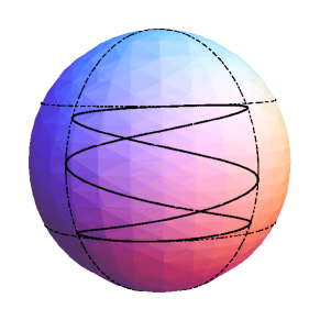
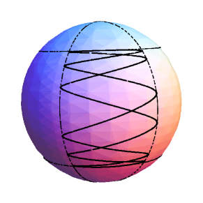
Figure 1: Plot of $(\phi,\theta)$-trajectories for $k=3$. The figure on the left is for the one–parameter PT potential $H_{\phi}$, $\omega_{\phi}=3\omega_{\theta}$. The right hand figure is for the two–parameter PT potential $\omega_{\phi}=6\omega_{\theta}$ (right). These trajectories are inscribed on ‘spherical rectangles’ (dashing curves).

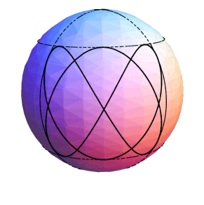
Figure 2: Plot of $(\phi,\theta)$-trajectories for $k=2/3$, $3\omega_{\phi}=2\omega_{\theta}$ (left) and $k=4/5$, $5\omega_{\phi}=4\omega_{\theta}$ (right) of the one–parameter PT system inscribed in ‘spherical rectangles’ (dashing curves).

Figure 3: Plot of same trajectories for $k=2/3$ (left) and $k=4/5$ (right) as in Fig. 2 but in ‘true’ spherical coordinates $(\varphi,\theta)$.

5 Conclusions

The kind of quantum systems we have considered in this paper are characterized by a separation of variables, such that for each variable they give rise to factorizable one–dimensional systems. The factorization properties of these one–dimensional component systems allow the construction of nontrivial symmetries. We have shown in our example how this process is carried out and the way that the symmetries can be applied to find the degeneracy of the energy levels. Although these symmetries are non polynomial, they can directly lead us to the polynomial ones [14].

We have called Lissajous systems to the corresponding classical systems due to similarities of their trajectories with the Lissajous curves. These classical systems keep the same separation properties giving rise to one–dimensional classical systems. Although it is not well known, a whole class of classical one–dimensional systems have analogue factorization properties as their quantum counterparts [13]. This type of classical factorizations is important, for instance, in the search of action–angle variables, or in the study of the correspondence of classical and quantum properties through coherent states [19]. By using these classical factorization properties we have shown how to get the symmetries of the classical system in the same way as in the quantum case. From the symmetries it is obtained the ratio of frequencies of the periodic motion in each variable as well as the rectangles where the trajectories are inscribed. The explicit computation of the time–dependence and the frequency of the motion in one of the variables is done through the ladder functions of the corresponding one–dimensional system. In this way, the picture of the system is complete from an algebraic point of view.

This method to search the symmetries of classical and quantum systems was advocated in [10] as a different way to that followed in previous references [1]-[9]. In general, in such references the solutions of the Hamilton–Jacobi equation are used in order to find the classical constants of motion. In the quantum case, it is the solutions of the Schrödinger equation which are used to get recurrence relations and from here, the symmetry operators. We have not used any solution at all, but only the algebraic properties of the quantum or classical Hamiltonians.

We have restricted ourselves in this paper to a very simple case on the sphere. Our aim is just to introduce our method in the most clear way and to show the main applications and advantages. A thorough systematic classification of the Lissajous systems is in progress.

Acknowledgments

We acknowledge financial support from GIR of Mathematical Physics of the University of Valladolid. Ş. Kuru acknowledges the warm hospitality at Department of Theoretical Physics, University of Valladolid, Spain.

References

- [1] F. Tremblay, A.V. Turbiner and P. Winternitz, J. Phys. A: Math. Theor. 42 (2009) 242001.
- [2] F. Tremblay, A.V. Turbiner and P. Winternitz, J. Phys. A: Math. Theor. 43 (2010) 015202.
- [3] E.G. Kalnins, J.M. Kress and W. Miller Jr., J. Phys. A: Math. Theor. 43 (2010) 265205.
- [4] E.G. Kalnins, J.M. Kress and W. Miller Jr., SIGMA 6 (2010) 066.
- [5] S. Post and P. Winternitz, J. Phys. A: Math. Theor. 43 (2010) 222001.
- [6] E.G. Kalnins and W. Miller Jr., J. Nonl. Sys. App. (2012) 29.
- [7] M. F. Rañada, J. Phys. A: Math. Theor. 45 (2012) 465203.
- [8] M. F. Rañada, J. Phys. A: Math. Theor. 46 (2013) 125206.
- [9] D. Lévesque, S. Post and P. Winternitz, J. Phys. A: Math. Theor. 45 (2012) 465204.
- [10] E. Celeghini, Ş. Kuru, J. Negro and M.A. del Olmo, Ann. Phys. 332 (2013) 27.
- [11] E. Schrödinger, Proc. Roy. Irish Acad. 46 (1941) 9; 46 (1941) 183.
- [12] L. Infeld and T.E. Hull, Rev. Mod. Phys. 23 (1951) 21.
- [13] Ş. Kuru and J. Negro, Ann. Phys. 323 (2008) 413.
- [14] J.A. Calzada, Ş. Kuru and J. Negro, Polynomial symmetries of spherical Lissajous systems, Submitted.
- [15] F. J. Herranz and A. Ballesteros, SIGMA 2 (2006) 010.
- [16] A. Ballesteros, F. J. Herranz and F. Musso, Nonlinearity 26 (2013) 971.
- [17] J.A. Calzada, Ş. Kuru, J. Negro and M.A. del Olmo, Ann. Phys. 327 (2012) 808.
- [18] Ş. Kuru and J. Negro, Ann. Phys. 324 (2009) 2548.
- [19] Ş. Kuru and J. Negro, Phys. Lett. A 376 (2012) 260.