Time Petri Nets with Dynamic Firing
Dates: Semantics and Applications

Abstract

We define an extension of time Petri nets such that the time at which a transition can fire, also called its firing date, may be dynamically updated. Our extension provides two mechanisms for updating the timing constraints of a net. First, we propose to change the static time interval of a transition each time it is newly enabled; in this case the new time interval is given as a function of the current marking. Next, we allow to update the firing date of a transition when it is persistent, that is when a concurrent transition fires. We show how to carry the widely used state class abstraction to this new kind of time Petri nets and define a class of nets for which the abstraction is exact. We show the usefulness of our approach with two applications: first for scheduling preemptive task, as a poor man’s substitute for stopwatch, then to model hybrid systems with non trivial continuous behavior.

1 Introduction

A Time Petri Net [15, 6] (TPN) is a Petri net where every transition is associated to a static time interval that restricts the date at which a transition can fire. In this model, time progresses with a common rate in all the transitions that are enabled; then a transition $t$ can fire if it has been continuously enabled for a time $\theta_{t}$ and if the value of $\theta_{t}$ is in the static time interval, denoted $\textbf{I}_{s}(t)$. The term static time interval is appropriate in this context. Indeed, the constraint is immutable and do not change during the evolution of the net. In this paper, we lift this simple restriction and go one step further by also updating the timing constraint of persistent transitions, that is transitions that remain enabled while a concurrent transition fires. In a nutshell, we define an extension of TPN where the time at which a transition can fire, also called its firing date, may be dynamically updated. We say that these transitions are fickle and we use the term Dynamic TPN to refer to our extension.

Our extension provides two mechanisms for updating the timing constraints of a net. First, we propose to change the static time interval of a transition each time it is newly enabled. In this case the new time interval $\textbf{I}_{s}(t,m)$ is obtained as a function of the current marking $m$ of the net. Likewise, we allow to update the deadline of persistent transitions using an expression of the form $\textbf{I}_{d}(t,m,\varphi_{t})$, that is based on the previous firing date of $t$. The first mechanism is straightforward and quite similar to an intrinsic capability of Timed Automata (TA); namely the possibility to compare a given clock to different constants depending on the current state. Surprisingly, it appears that this extension has never been considered in the context of TPN. The second mechanism is far more original. To the best of our knowledge, it has not been studied before in the context of TPN or TA, but there are some similarities with the updatable timed automata of Bouyer et al. [9].

The particularity of timed models, such as TPN, is that state spaces are typically infinite, with finite representations obtained by some abstractions of time. In the case of TPN, states are frequently represented using composite abstract states, or state classes, that captures a discrete information (e.g. the marking) together with a timing information (represented by systems of difference constraints or zones). We show how to carry the state class abstraction to our extended model of TPN. We only obtain an over-approximation of the state space in the most general case, but we define a class of nets for which the abstraction is exact. We conjecture that our approach could be used in other formal models for real-time systems, such as timed automata for instance.

There exist several tools for reachability analysis of TPN based on the notion of state class graph [5, 3], like for example Tina [7] or Romeo [14]. Our construction provides a simple method for supporting fickle transitions in these tools. Actually, our extension has been implemented inside the tool Tina in a matter of a few days. We have used this extension of Tina to test the usefulness of our approach in the context of two possible applications: first for scheduling preemptive task, as a poor man’s substitute for stopwatch; next to model dynamical systems with non trivial continuous behavior.

Outline of the paper and contributions.

We define the semantics of TPN with dynamic firing dates in Sect. 2. We prove that we directly subsume the class of “standard” TPN and that our extension often leads to more concise models. In Sect. 2.3, we motivate our extension by showing how to implement the Quantized State System (QSS) method [10]. This application underlines the advantage of using an asynchronous approach when modeling hybrid systems. Section 3 provides an incremental construction for the state class graph of a dynamic TPN. Before concluding, we give some experimental results for two possible applications of dynamic TPN.

2 Time Petri nets and Fickle Transitions

A Time Petri net is a Petri net where transitions are decorated with static time intervals that constrain the time a transition can fire. We denote $\mathbb{I}$ the set of possible time intervals. We use a dense time model in our definitions, meaning that we choose for $\mathbb{I}$ the set of real intervals with non negative rational end-points. To simplify the definitions, we only consider the case of closed intervals, $[a,b]$, and infinite intervals of the form $[a,+\infty)$. For any interval $i$ in $\mathbb{I}$, we use the notation ${\downarrow}i$ for its left end-point and ${\uparrow}i$ for its right end-point (or $\infty$ if $i$ is unbounded).

We use the expression Dynamic TPN (DTPN) when it is necessary to make the distinction between our model and more traditional definitions of TPN. With our notations, a dynamic TPN is a tuple $\langle{P},{T},{\mathbf{Pre}},{\mathbf{Post}},m_{0},\textbf{I}_{s},\textbf{I}_{d}\rangle$ in which:

• $\langle{P},{T},{\mathbf{Pre}},{\mathbf{Post}},m_{0}\rangle$ is a Petri net, with ${P}$ the set of places, ${T}$ the set of transitions, $m_{0}:P\rightarrow\mathbb{N}$ the initial marking, and ${\mathbf{Pre}},\leavevmode\nobreak\ {\mathbf{Post}}:{T}\rightarrow{P}\rightarrow\mathbb{N}$ the precondition and postcondition functions.

• $\textbf{I}_{s}$ is the static interval function, that associates a time interval (in $\mathbb{I}$) to every transition (in $T$).

• $\textbf{I}_{d}$ is the dynamic interval function. It will be used to update the firing date of persistent transitions.

We slightly extend the “traditional” model of TPN and allow to define the static time interval of a transition as a function of the markings, meaning that $\textbf{I}_{s}$ is a function of $T\to(P\to\mathbb{N})\to\mathbb{I}$. We will often used the curryied function $\textbf{I}_{s}(t)$ to denote the mapping from a marking $m$ to the time interval $\textbf{I}_{s}(t,m)$.

We also add the notion of dynamic interval function, $\textbf{I}_{d}$, that is used to update the firing date of persistent transitions. The idea is to update the firing date $\varphi_{t}$ of a persistent transition $t$ using a function of $\varphi_{t}$. Hence $\textbf{I}_{d}$ is a function of $T\to(P\to\mathbb{N})\to\mathbb{R}_{\geq 0}\to\mathbb{I}$. For example, a transition $t$ such that $\textbf{I}_{d}(t,m,\theta)=[\theta+1,\theta+2]$, for all $\theta\geq 0$, models an event that is delayed by between $1$ and $2$ unit of time (u.t.) when a concurrent transition fires.

2.1 A Semantics for Time Petri Nets Based on Firing Functions

As usual, we define a marking $m$ of a TPN as a function $m:{P}\rightarrow\mathbb{N}$ from places to integers. A transition $t\in{T}$ is enabled at $m$ if and only if $m\geq\mathbf{Pre}(t)$ (we use the pointwise comparison between functions). We denote ${\cal E}(m)$ the set of transitions enabled at $m$.

A state of a TPN is a pair $s=(m,\varphi)$ in which $m$ is a marking and $\varphi:{T}\rightarrow\mathbb{R}_{\geq 0}$ is a mapping, called the firing function of $s$, that associates a firing date to every transition enabled at $m$. Intuitively, if $t$ is enabled at $m$, then $\varphi_{t}$ is the date (in the future, from now) at which $t$ should fire. Also, the transitions that may fire from a state $(m,\varphi)$ are exactly the transitions $t$ in ${\cal E}(m)$ such that $\varphi_{t}$ is minimal; they are the first scheduled to fire.

For any date $\theta$ in $\mathbb{R}_{\geq 0}$, we denote $\varphi\mathbin{\text{\ooalign{\raise 4.30554pt\hbox{.}\cr$-$\cr}}}\theta$ the partial function that associates the transition $t$ to the value $\varphi_{t}-\theta$, when $\varphi_{t}\geq\theta$, and that is undefined elsewhere. This operation is useful to model the effect of time passage on the enabled transitions of a net. We say that the firing function $\varphi\mathbin{\text{\ooalign{\raise 4.30554pt\hbox{.}\cr$-$\cr}}}\theta$ is well-defined if it is defined on exactly the same transitions than $\varphi$.

The following definitions are quite standard. The semantics of a TPN is a Kripke structure $\langle S,S_{0},\rightarrow\rangle$ with only two possible kind of actions: either $s\mathbin{\smash{\overset{{t}}{{\to}}}}s^{\prime}$ (meaning that the transition $t\in T$ is fired from $s$); or $s\mathbin{\smash{\overset{{\theta}}{{\to}}}}s^{\prime}$, with $\theta\in\mathbb{R}_{\geq 0}$ (meaning that we let time $\theta$ elapse from $s$). A transition $t$ may fire from the state $(m,\varphi)$ if $t$ is enabled at $m$ and firable instantly (that is $\varphi_{t}=0$). In a state transition $(m,\varphi)\mathbin{\smash{\overset{{t}}{{\to}}}}(m^{\prime},\varphi^{\prime})$, we say that a transition $k$ is persistent (with $k\neq t$) if it is also enabled in the marking $m-\mathbf{Pre}(t)$, that is if $m-\mathbf{Pre}(t)\geq\mathbf{Pre}(k)$. The transitions that are enabled at $m^{\prime}$ and not at $m$ are called newly enabled. We define the predicates $\operatorname{prs}$ and $\operatorname{nbl}$ that describe the set of persistent and newly enabled transitions after $t$ fires from $m$:

$$\begin{array}[]{lcl}\operatorname{prs}(m,t)&=&\{k\in{\cal E}(m)\mid m-\mathbf{Pre}(t)\geq\mathbf{Pre}(k)\}\\ \operatorname{nbl}(m,t)&=&\{k\in(T\setminus{\cal E}(m))\cup\{t\}\mid m-\mathbf{Pre}(t)+\mathbf{Post}(t)\geq\mathbf{Pre}(k)\}\end{array}$$

We use these two predicates to define the semantics of DTPN.

Definition 1.

The semantics of a DTPN $\langle{P},{T},{\mathbf{Pre}},{\mathbf{Post}},m_{0},\textbf{I}_{s},\textbf{I}_{d}\rangle$ is the timed transition system $SG=\langle S,S_{0},\rightarrow\rangle$ such that:

• $S$ is the set of states of the TPN;

• $S_{0}$, the set of initial states, is the subset of states of the form $(m_{0},\varphi)$, where $m_{0}$ is the initial marking and $\varphi_{t}\in\textbf{I}_{s}(t,m_{0})$ for every $t$ in ${\cal E}(m_{0})$;

• the state transition relation ${\rightarrow}\subseteq S\times({{T}\cup\mathbb{R}_{\geq 0}})\!\times S$ is the smallest relation such that for all state $(m,\varphi)$ in $S$:

  • if $t$ is enabled at $m$ and $\varphi_{t}=0$ then $(m,\varphi)\mathbin{\smash{\overset{{t}}{{\to}}}}(m^{\prime},\varphi^{\prime})$ where $m^{\prime}=m-\mathbf{Pre}(t)+\mathbf{Post}(t)$ and $\varphi^{\prime}$ is a firing function such that $\varphi_{k}^{\prime}\in\textbf{I}_{d}(k,m^{\prime},\varphi_{k})$ for all persistent transition $k\in\operatorname{prs}(m,t)$ and $\varphi_{k}^{\prime}\in\textbf{I}_{s}(k,m^{\prime})$ otherwise.

  • if $\varphi\mathbin{\text{\ooalign{\raise 4.30554pt\hbox{.}\cr$-$\cr}}}\theta$ is well-defined then $(m,\varphi)\mathbin{\smash{\overset{{\theta}}{{\to}}}}(m,\varphi\mathbin{\text{\ooalign{\raise 4.30554pt\hbox{.}\cr$-$\cr}}}\theta)$.

The state transitions labelled over $T$ (case $(i)$ above) are the discrete transitions, those labelled over $\mathbb{R}_{\geq 0}$ (case $(ii)$) are the continuous, or time elapsing, transitions. It is clear from Definition 1 that, in a discrete transition $(m,\varphi)\mathbin{\smash{\overset{{t}}{{\to}}}}(m^{\prime},\varphi^{\prime})$, the transitions enabled at $m^{\prime}$ are exactly $\operatorname{prs}(m,t)\cup\operatorname{nbl}(m,t)$. In the target state $(m^{\prime},\varphi^{\prime})$, a newly enabled transition $k$ get assigned a firing date picked “at random” in $\textbf{I}_{s}(k,m^{\prime})$. Similarly, a persistent transition $k$ get assigned a firing date in $\textbf{I}_{d}(k,m^{\prime},\varphi_{k})$. Because there may be an infinite number of transitions, the state spaces of TPN are generally infinite, even when the net is bounded. This is why we introduce an abstraction of the semantics in Sect. 3.

We can define two simple extensions to DTPN. First, we can use a special treatment for re-initialized transitions; transitions that are enabled before $t$ fires and newly-enabled after. In this case we could use the previous firing date to compute the static interval. Then, in the interval functions $\textbf{I}_{d}$ and $\textbf{I}_{s}$, we can use the “identifier” of the transition that fires in addition to the target marking, $m^{\prime}$. These extensions preserve the results described in this paper

Our definitions differ significantly from the semantics of TPN generally used in the literature. For instance, in the works of Berthomieu et al. [1], states are either based on clocks—that is on the time elapsed since a transition was enabled—or on firing domains (also called time zones)—that abstract the sets of possible “time to fire” using intervals. Our choice is quite close to the TPN semantics based on firing domains (in particular we have the same set of traces) and is similar in spirit to the semantics used by Vicario et al. [18] for reasoning about Stochastic Time Petri nets. We made the choice of an unorthodox semantics to simplify our definition of firing date. We conjecture that most of our definitions can be transposed to a clock-based semantics.

2.2 Interesting Classes of DTPN

In the standard semantics of TPN [15], the firing date of a persistent transition is left unchanged. We can obtain a similar behavior by choosing for $\textbf{I}_{d}(t,m,\theta)$ the time interval $[\theta,\theta]$. We say in this case that the dynamic interval function is trivial. Another difference with respect to the standard definition of TPN is the fact that the (static!) time interval of a transition may change. We say that a dynamic net is a TPN if its static function, $\textbf{I}_{s}$, is constant and its dynamic function, $\textbf{I}_{d}$, is trivial. We say that a DTPN is weak if only the function $\textbf{I}_{d}$ is trivial. We show that TPN are as expressive than weak DTPN when the nets are bounded. Weak nets are still interesting though, since the use of non-constant interval functions can lead to more concise models. On the other hand, the results of Sect. 3 show that, even in bounded nets, fickle transitions are more expressive than weak ones.

Theorem 1.

For every weak DTPN that has a finite set of reachable markings, there is a TPN that has an equivalent semantics.

Proof.

see Appendix A. ∎

We define a third class of nets, called translation DTPN, obtained by restricting the dynamic interval function $\textbf{I}_{d}$. This class arises naturally during the definition of the State Class Graph construction in Sect. 3. Intuitively, with this restriction, a persistent transition can only shift its firing date by a “constant time”. The constant can be negative and may be a function of the marking. More precisely, we say that a DTPN is a translation if, for every transitions $t$, there are two functions $\kappa_{1}$ and $\kappa_{2}$ from $(P\to\mathbb{N})\to\mathbb{Q}$ such that ${\textbf{I}_{d}(t,m,\theta)}$ is the time interval $[A,B]$ where $A=\max(0,\theta+\kappa_{1}(m))$ and $B=\max(A,\theta+\kappa_{2}(m))$. (The use of $\max$ in the definition of $A,B$ is necessary to accomodate negative constants $\kappa_{i}(m)$.)

2.3 Interpretation of the Quantized State System Model

With the addition of fickle transitions, it is possible to model systems where the timing constraints of an event depend on the current state. This kind of situations arises naturally in practice. For instance, we can use the function $\textbf{I}_{s}$ to model the fact that the duration of a communication depends on the length of a message. Likewise, we can use the fickle function $\textbf{I}_{d}$ when modeling the typical workflow of a conference, in which a deadline may be postponed when particular events occurs.

In this section, we consider a simple method for analyzing the behavior of a system with one continuous variable, $x$, governed by the ordinary differential equation $\dot{x}=f(x)$. The idea is to define a TPN that computes the value $x(\theta)$ of the variable $x$ at the date $\theta$. To this end, we use an extension of TPN with shared variables, $x,y,\dots$, where every transition may be guarded by a boolean predicate (on $b$) and such that, upon firing, a transition can update the environment (using a sequence of assignments, do $e$). This extension of TPN with shared variables can already be analyzed using the tool Tina.

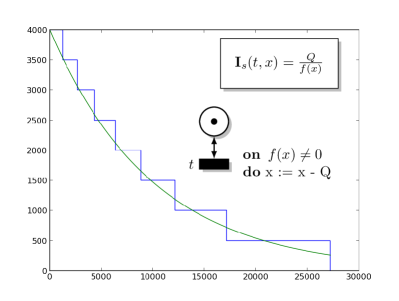
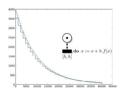
Figure 1: A simple QSS simulation (left) and the Euler method (right) for $\dot{x}=-x$. ($Q=500$, $h=1150$, global error smaller than $500$.)

The simplest solution is based on the Euler forward method. This is modeled by the TPN of Fig. 1 (right) that periodically execute the instruction $x:=x+h.f(x)$ every $h$ (the value of the time step, $h$, is the only parameter of the method). This solution is a typical example of synchronous system, where we sample the evolution of time using a “quantum of time”. A synchronous approach answers the following question: given the value of $x$ at time $k.h$, what is its value at time $(k+1).h$?

The second solution is based on the Quantized State System (QSS) method [10, 11], which can be interpreted as the dual—the asynchronous counterpart—of the Euler method. QSS uses a “quantum of value”, $Q$, meaning that we only consider discrete values for $x$, of the form $k.Q$ with $k\in\mathbb{N}$. The idea is to compute the time necessary for $x$ to change by an amount of $Q$. To paraphrase [11], the QSS method answers the following modified question: given that $x$ has value $k.Q$, what is the earliest time at which $x$ has value $(k\pm 1).Q$? This method has a direct implementation using fickle transitions: at first approximation, the time $\varphi_{t}$ for $x$ to change by an amount of $Q$ is given by the relation $(x\pm Q)=x+\varphi_{t}.f(x)$, that is $\varphi_{t}=\nicefrac{{Q}}{{|f(x)|}}$. We have that the time slope of $x$ is equal to $\nicefrac{{1}}{{f(x)}}$. The role of the guard $f(x)\neq 0$ on transition $t$ is to avoid pathological values for the slope; when $f(x)$ is nil the value of $x$ stays constant, as needed.

We compare the results obtained with these two different solutions in Fig. 1, where we choose $f(x)=-x$ and $x(0)=4000$. Each plot displays the evolution of the TPN compared to the analytic solution, in this case $x(\theta)=4000e^{-\theta}$. Numerical methods are of course approximate; in both cases (Euler and QSS) the global error is proportional to the quantum. The plots are obtained with the largest quantum values giving a global error smaller than $500$, that is a step $h$ of $1150$ and a quantum $Q$ of $500$. The dynamic TPN has $10$ states while the standard TPN has $38$. The ratio improves when we try to decrease the global error. For instance, for an error smaller than $100$ (which gives $Q=100$ and $h=250$) we have $42$ states against $182$. We observe that in this case the “asynchronous” solution is more concise than the synchronous one.

The Euler method is the simplest example in a large family of iterative methods for approximating the solutions of differential equations. The QSS method used in this section can be enhanced in just the same way, leading to more precise solutions, with better numerical stability. Some of the improved QSS methods have been implemented in our tool, but we still experiment the effect of numerical instability on some stiff systems. In these cases, the synchronous approach (that is deterministic) may sometimes exhibit better performances.

Although we make no use of the fickle function $\textbf{I}_{d}$ here, it arises naturally when the system has multiple variables. Consider a system with two variables, $x,y$, such that $x=f(x,y)$. We can use the same solution than in Fig. 1 to model the evolution of $x$ and $y$. When the value of $x$ just changes, the next update is scheduled at the date $\nicefrac{{Q}}{{f(x,y)}}$ (the time slope is $f_{1}=\nicefrac{{1}}{{f(x,y)}}$). If the value of $y$ is incremented before this deadline—say that the remaining time if $\theta_{1}$—we need to update the time slope and use the new value $f_{2}=\nicefrac{{1}}{{f(x,y+Q)}}$.

Figure 2: Computing the updated firing date in the QSS method.

We illustrate the situation in the two diagrams of Fig. 2, where we assume that $f_{1}$ is positive. For instance, if the two slopes have the same sign (diagram to the left), we need to update the firing date to the value $\theta_{2}$ such that $|f_{1}|.\theta_{1}=|f_{2}|.\theta_{2}$. Likewise, when $f_{2}$ is negative, we have the relation $|f_{1}|.\theta_{1}+|f_{2}|.\theta_{2}=2.Q$. Therefore, depending on the sign of $f_{1}.f_{2}$ (the sign of $\dot{y}$ tell us whether $y$ is incremented or decremented) we have $\textbf{I}_{d}(t,x,y,\theta)=[A(\theta),A(\theta)]$ with:

$$A(\theta)=\frac{|f(x,y\pm Q)|}{|f(x,y)|}.\theta\qquad\text{ or }\qquad\frac{|f(x,y\pm Q)|}{|f(x,y)|}.\left(2.Q.|f(x,y)|-\theta\right)$$

This example shows that it is possible to implement the QSS method using only linear fickle functions. (We discuss briefly the associated class of DTPN at the end of Sect. 3.) Since the notion of slope is central in our implementation of the QSS method, we could have used instead an extension of TPN with multirate transitions [12], that is a model where time advance at different rate depending on the state. While the case $f_{1}.f_{2}>0$ lends itself well to this extension, it is not so obvious when the slopes have different signs. On the opposite, it would be interesting to use fickle transitions as a way to mimic multirate transitions.

3 A State Class Abstraction for Dynamic TPN

In this section, we generalize the state class abstraction method to the case of DTPN. A State Class Graph ($SCG$) is a finite abstraction of the timed transition system of a net that preserves the markings and traces. The construction is based on the idea that temporal information in states (the firing functions) can be conveniently represented using systems of difference constraints [17]. We show that the $SCG$ faithfully abstract the semantics of a net when the dynamic interval functions are translations. We only over-approximate the set of reachable markings in the most general case.

A state class $C$ is defined by a pair $(m,D)$, where $m$ is a marking and the firing domain $D$ is described by a (finite) system of linear inequalities. We say that two state classes $C=(m,D)$ and $C^{\prime}=(m^{\prime},D^{\prime})$ are equal, denoted $C\cong C^{\prime}$, if $m=m^{\prime}$ and $D\Leftrightarrow D^{\prime}$ (i.e. $D$ and $D^{\prime}$ have equal solution sets). Hence class equivalence is decidable. In a domain $D$, we use variables $x_{t},y_{t},\dots$ to denote a constraint on the value of $\varphi_{t}$. A domain $D$ is defined by a set of difference constraints in reduced form: $\alpha_{i}\leq x_{i}\leq\beta_{i}$ and $x_{i}-x_{j}\leq\gamma_{i,j}$, where $i,j$ range over a given subset of “enabled transitions” and the coefficients $\alpha,\beta$ and $\gamma$ are rational numbers. We can improve the reduced form of $D$ by choosing the tightest possible bounds that do not change its associated solutions set. In this case we say that D is in closure form. We show in Th. 2 how to compute the coefficients of the closure form incrementally.

In the remainder of this section, we use the notation $A^{s}_{t}(m)$ and $B^{s}_{t}(m)$ for the left and right endpoints of $\textbf{I}_{s}(t,m)$. Likewise, when the marking $m$ is obvious from the context, we use the notations $A_{t}(\theta)$ and $B_{t}(\theta)$ for the left and right endpoints of $\textbf{I}_{d}(t,m,\theta)$, that is $A_{t}(\theta)={\downarrow}\textbf{I}_{d}(t,m,\theta)$ and $B_{t}(\theta)={\uparrow}\textbf{I}_{d}(t,m,\theta)$. We call $A_{t}$ and $B_{t}$ the fickle functions of $t$. In the remainder of the text, we assume that $0\leq A_{t}(\theta)\leq B_{t}(\theta)$ for all possible (positive) date $\theta$ and that $A(\infty)=\infty$. We also require these functions to be monotonically increasing. We impose no other restrictions on the fickle functions.

We define inductively a set of classes $C_{\sigma}$, where $\sigma\in T^{*}$ is a sequence of discrete transitions firable from the initial state. This is the State Class Graph construction of [5, 3]. Intuitively, the class $C_{\sigma}=(m,D_{\sigma})$ “collects” the states reachable from the initial state by firing schedules of support sequence $\sigma$. The initial class $C_{\epsilon}$ is $(m_{0},D_{0})$ where $D_{0}$ is the domain defined by the set of inequalities $A^{s}_{i}(m_{0})\leq x_{i}\leq B^{s}_{i}(m_{0})$ for all $i$ in ${\cal E}(m_{0})$.

Assume $C_{\sigma}=(m,D)$ is defined and that $t$ is enabled at $m$. We details how to compute the domain for the class $C_{\sigma.t}$. First we test whether the system $D$ extended with the constraints $D_{t}=\{x_{k}-x_{t}\geq 0\mid t\neq k,k\in{\cal E}(m)\}$ is consistent. This is in order to check that transition $t$ can be fired before any other enabled transitions $k$ at $m$. If $D\wedge D_{t}$ is consistent, we add $C_{\sigma.t}=(m^{\prime},D^{\prime})$ to the set of reachable classes, where $m^{\prime}$ is the result of firing $t$ from $m$, i.e. $m^{\prime}=m-\mathbf{Pre}(t)+\mathbf{Post}(t)$. The computation of $D^{\prime}$ follows the same logic than with standard TPN.

We choose a set of fresh variables, say $y_{k}$, for every transition $k$ that is enabled at $m^{\prime}$. For every persistent transition, $k\in\operatorname{prs}(m,t)$, we add the constraints $x_{k}=y_{k}-x_{t}$ to the set of inequalities in $D\wedge D_{t}$. The variable $y_{k}$ matches the firing date of $k$ at the time $t$ fires, that is, the value of $\varphi_{k}$ used in the expression $\textbf{I}_{d}(k,m^{\prime},\varphi_{k})$ (see Definition 1, case $(i)$). For every newly enabled transition, $k\in\operatorname{nbl}(m,t)$, we add the constraints $A^{s}_{k}(m^{\prime})\leq y_{k}\leq B^{s}_{k}(m^{\prime})$. This constraint matches the fact that $\varphi_{k}^{\prime}$ is in the interval $\textbf{I}_{s}(k,m^{\prime})$ if $k$ is newly enabled at $m^{\prime}$. As a result, we obtain a set of inequations where we can eliminate all occurrences of the variables $x_{k}$ and $x_{t}$. After removing redundant inequalities and simplifying the constraints on transitions in conflicts with $t$—so that the variables only ranges over transitions enabled at $m^{\prime}$—we obtain an “intermediate” domain $D_{\mathit{int}}$ that obeys the constraints: $\kappa_{i}\leq y_{i}\leq\lambda_{i}$ and $y_{i}-y_{j}\leq\mu_{i,j}$, where $i,j$ range over ${\cal E}(m^{\prime})$ and the constants $\kappa,\lambda$ and $\mu$ are defined as follows.

$$\begin{array}[c]{lcl@{\quad}l}\kappa_{i}&=&\left\{\begin{array}[c]{l}A^{s}_{i}(m^{\prime})\\ \max\,(0,\{-\gamma_{i,j}\mid{i,j\in{\cal E}(M)}\})\\ \end{array}\right.&\begin{array}[c]{l}\text{if $i$ is newly enabled,}\\ \text{otherwise}\end{array}\\[10.00002pt] \lambda_{i}&=&\left\{\begin{array}[c]{l}B^{s}_{i}(m^{\prime})\\ \gamma_{i,t}\\ \end{array}\right.&\begin{array}[c]{l}\text{if $i$ is newly enabled,}\\ \text{otherwise}\end{array}\\[10.00002pt] \mu_{i,j}&=&\left\{\begin{array}[c]{l}\lambda_{i}-\kappa_{j}\\ \min\,(\gamma_{i,j},\lambda_{i}-\kappa_{j})\\ \end{array}\right.&\begin{array}[c]{l}\text{if either $i$ or $j$ newly enabled,}\\ \text{otherwise}\\ \end{array}\end{array}$$

Finally, we need to apply the effect of the fickle functions. For this, we rely on the fact that $A_{i}$ and $B_{i}$ are monotonically increasing functions. To obtain $D^{\prime}$, we choose a set of fresh variables, say $x_{i}^{\prime}$, for every transition $i\in{\cal E}(m^{\prime})$ and add the following relations to $D_{\mathit{int}}$. To simplify the notation, we assume that in the case of a newly enabled transition, $j$, the functions $A_{j}$ and $B_{j}$ stand for the identity function (with this shorthand, we avoid to distinguish cases where both or only one of the transitions are persistent):

$$\begin{array}[c]{l@{\quad}l}x_{i}^{\prime}=y_{i}&\text{if $i,j$ are newly enabled}\\ A_{i}(y_{i})\leq x_{i}^{\prime}\leq B_{i}(y_{i})\text{\ and\ }x_{i}^{\prime}-x_{j}^{\prime}\leq B_{i}(y_{i})-A_{j}(y_{j})&\text{if $i$ or $j$ are persistent}\\ \end{array}$$

The relation for newly enabled transitions simply states that $y_{i}$ already captures all the constraints on the firing time $\varphi_{i}^{\prime}$. For persistent transitions, the first relation states that $x_{i}^{\prime}$ is in the interval $[A_{i}(y_{i}),B_{i}(y_{i})]$, that is in $\textbf{I}_{d}(i,m^{\prime},\varphi(i))$.

We obtain the domain $D^{\prime}$ by eliminating all the variables of the kind $y_{i}$. First, we can observe that, by monotonicity of the functions $A_{i}$ and $B_{i}$, we have $A_{i}(\kappa_{i})\leq A_{i}(y_{i})$ and $B_{i}(y_{i})\leq B_{i}(\lambda_{i})$. This gives directly a value for the coefficients $\alpha^{\prime}_{i}$ and $\beta^{\prime}_{i}$. The computation of the coefficient $\gamma^{\prime}_{i,j}$ is more complex, since it amounts to computing the maximum of a function over a convex sets of points. Indeed $\gamma^{\prime}_{i,j}$ is the least upper-bound for the values of $x_{i}^{\prime}-x_{j}^{\prime}$ over $D_{\mathit{int}}$ or, equivalently:

$$\begin{array}[]{lcl}\gamma^{\prime}_{i,j}&=&\max\,\{B_{i}(y_{i})-A_{j}(y_{j})\mid y_{i},y_{j}\in D_{\mathit{int}}\}\\ &=&\max\,\{B_{i}(y_{i})-A_{j}(y_{j})\mid\kappa_{i}\leq y_{i}\leq\lambda_{i},\kappa_{j}\leq y_{j}\leq\lambda_{j},y_{i}-y_{j}\leq\mu_{i,j}\}\\ \end{array}$$

It is possible to simplify the definition of $\gamma^{\prime}_{i,j}$. Indeed, if we fix the value of $y_{j}$ then, by monotonicity of $B_{i}$, the maximal value of $B_{i}(y_{i})-A_{j}(y_{j})$ is reached when $y_{i}$ is maximal. Hence we have two possible cases: either $(i)$ it is reached for $y_{i}=y_{j}+\mu_{i,j}$ if $\kappa_{j}\leq y_{j}\leq\lambda_{i}+\mu_{i,j}$; or $(ii)$ it is reached for $y_{i}=\lambda_{i}$ if $\lambda_{i}-\mu_{i,j}\leq y_{j}\leq\lambda_{j}$. This result is illustrated in the schema of Fig. 3a, where we display an example of domain $D_{\mathit{int}}$. When $y_{j}$ is constant (horizontal line), the maximal value is on the “right” border of the convex set (bold line). We also observe that in case $(ii)$, by monotonicity of $A_{j}$, the maximal value is equal to $B_{i}(\lambda_{i})-A_{j}(\lambda_{i}+\mu_{i,j})$. Therefore the value of $\gamma^{\prime}_{i,j}$is obtained by computing the maximal value of the expression $B_{i}(\theta)-A_{j}(\theta-\mu_{i,j})$, that is:

$$\gamma^{\prime}_{i,j}=\max\,\{B_{i}(\theta)-A_{j}(\theta-\mu_{i,j})\mid\kappa_{j}+\mu_{i,j}\leq\theta\leq\lambda_{i}\}$$

As a consequence, the value of $\gamma^{\prime}_{i,j}$ can be computed by finding the minimum of a numerical function (of one parameter) over a real interval, which is easy.

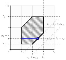
(a) Domain $D_{\mathit{int}}$ projected over $t_{i},t_{j}$

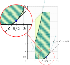
(b) Domain $D^{\prime}$ obtained from $D_{\mathit{int}}$

Figure 3: Computing the coefficient $\gamma^{\prime}_{i,j}$ in the domain $D^{\prime}$.

We display in Fig. 3b the domain $D^{\prime}$ obtained from $D_{\mathit{int}}$ after applying the fickle functions. In this example, $t_{j}$ is the only fickle transition and we choose $A_{j}(\theta)=B_{j}(\theta)=(\theta-\nicefrac{{1}}{{2}})^{2}$ when $\theta\geq\nicefrac{{1}}{{2}}$. With our method we have that $\mu_{i,j}=\nicefrac{{3}}{{2}}$ and the value of $\gamma^{\prime}_{i,j}$ is obtained by computing the maximal value of the expression $(\theta-\nicefrac{{1}}{{2}})^{2}-(\theta-\nicefrac{{3}}{{2}})$ with $\theta\in[2,3]$, that is $\nicefrac{{9}}{{4}}$.

Theorem 2.

Assume $C=(m,D)$ is a class with $D$ in closure form. Then for every transition $t$ in ${\cal E}(m)$ there is a unique class $(m^{\prime},D^{\prime})$ obtained from $C$ by firing $t$. The domain $D^{\prime}$ is also in closure form and can be computed incrementally as follows (we assume that $A_{i}$ and $B_{i}$ stands for the identity functions when $i$ is newly enabled).

$$\begin{array}[c]{lcl@{\quad}l}\alpha^{\prime}_{i}&=&A^{s}_{i}(m^{\prime})&\text{if $i$ is newly enabled,}\\ &=&\max\,(A_{i}(0),\{A_{i}(-\gamma_{i,j})\mid{i,j\in{\cal E}(M)}\})&\text{otherwise}\\ \beta^{\prime}_{i}&=&B^{s}_{i}(m^{\prime})&\text{if $i$ is newly enabled,}\\ &=&B_{i}(\gamma_{i,t})&\text{otherwise}\\ \gamma^{\prime}_{i,j}&=&\min(\gamma_{i,j},\beta^{\prime}_{i}-\alpha^{\prime}_{j})&\text{if $i,j$ are newly enabled,}\\ &=&\max\{B_{i}(\theta)-A_{j}(\theta-\mu_{i,j})\mid\mu_{i,j}+\kappa_{j}\leq x\leq\lambda_{i}\}&\text{otherwise}\\ \lx@intercol\hfil(\text{where }\lambda_{i},\kappa_{j}\text{ and }\mu_{i,j}\text{ are defined as in {(C1)}}\/)\lx@intercol\\ \end{array}$$

Moreover, if the state $(m,\varphi)$ is reachable in the state graph of a net, say $N$, and $(m,\varphi)\mathbin{\smash{\overset{{\theta}}{{\to}}}}\mathbin{\smash{\overset{{t}}{{\to}}}}(m^{\prime},\varphi^{\prime})$ then there is a class $C_{\sigma}=(m,D)$ reachable in the $SCG$ computed for $N$ with $\varphi\in D$, $C_{\sigma.t}=(m^{\prime},D^{\prime})$ and $\varphi^{\prime}\in D^{\prime}$.

The hatched area inside the domain displayed in Fig. 3b is the image of the domain $D_{\mathit{int}}$ after its transformation by the fickle function $A_{j}(\theta)$. We see that some points of $D^{\prime}$ have no corresponding states in $D_{\mathit{int}}$. Hence we only have an over-approximation. (We do not have enough place to give an example of net with a marking that is in reachable in the $SCG$ but not reachable in the state space, but such an example is quite easy to build.) If we consider the definition of the coefficients $\gamma^{\prime}$ in equation (C2), we observe that the situation is much simpler if the fickle functions are translations. Actually, it is possible to prove that, in this case, the $SCG$ construction is exact.

Theorem 3.

If the DTPN $N$ is a translation then the $SCG$ defined in Th. 2 has the same set of reachable markings and the same set of traces than the timed transition system of $N$.

sketch.

By equation (C2), if the net is a translation then there are two constants $c_{i},c_{j}$ such that $B_{i}(\theta)=\theta+c_{i}$ and $A_{j}(\theta)=\theta+c_{j}$. Therefore the expression $B_{i}(\theta)-A_{j}(\theta-\mu_{i,j})$ is constant and equal to $c_{i}-c_{j}-\mu_{i,j}$ (the maximum is reached all over the boundary of the domain). In this case, every state in $D^{\prime}$ has a corresponding states in $D_{\mathit{int}}$. ∎

We can also observe that, if the dynamic interval bounds $A_{i}$ and $B_{i}$ are linear functions, then we can follow a similar construct using (general) systems of inequations for the domains instead of difference constraints. This solution gives also an exact abstraction for the state space but is not interesting from a computational point of view (since we loose the ability to compute a canonical form for the domain incrementally). In this case, we are in a situation comparable to the addition of stopwatch to TPN where systems of difference constraints are not enough to precisely capture state classes. With our computation of the coefficient $\gamma^{\prime}$, see equation (C2), we use instead the “best difference bound matrix” that contains the states reachable from the class $C$. This approximation is used in some tools that support stopwatches, like Romeo [14].

4 Two Application for Dynamic TPN

We study two possible applications for fickle transitions. First to model a system of preemptive, periodic tasks with fixed duration. Next to model hybrid system with non trivial continuous behavior. These experiments have been carried out using a prototype extension of Tina. The tool and the all the models are available online at http://projects.laas.fr/tina/fickle/.

4.1 Scheduling Preemptive Tasks

We consider a simple system consisting of two periodic tasks, Task1 and Task2, executing on a single processor. Task2 has a period of $10$ unit of time (u.t.) and a duration of $6$ u.t. ; Task1 has a period of $5$ u.t. and a duration of $1$ and can preempt Task2 at any time. We display in Fig. 4 a TPN model for this system. Our model makes use of a stopwatch arc, drawn using an “open box” arrow tip ($\rule[2.0pt]{10.00002pt}{0.5pt}\mkern-3.0mu{\boxempty}$), and of an inhibitor arc ($\rule[2.0pt]{10.00002pt}{0.5pt}\mkern-3.0mu{\ocircle}$).

The net is the composition of four components. The roles of Sched1 and Sched2 is is to provide a token in place psched at the scheduling date of the tasks. The behavior of the nets corresponding to Task1 and Task2 are similar. Both nets are $1$-safe and their (unique) token capture the state of the tasks. When the token is in place e, the task execute; when it is in place w it is waiting for its scheduling event. Hence we have a scheduling error if there is a token in place psched and not in place w.

Figure 4: System with one preemptive and one simple task.

We use an inhibitor arc between the place e1 and the transition Task2Scheduled to model the fact that Task2 cannot use the processor if Task1 is already running. We use a stopwatch arc between e1 and the transition Task2Finished to model the fact that Task1 can preempt Task2 at any moment. A stopwatch (inhibitor) arc “freezes” the firing date of its transition. Therefore the completion of Task2 (the firing date of Task2Finished) is postponed as long as Task1 is running. Using the same approach, we can define a TPN modeling a system with one preemptive task and $n$ “simple”tasks.

We can define an equivalent model using fickle transitions instead of stopwatch. The idea is to add the duration of Task1 to the completion date of Task2 each time Task1 starts executing (that is Task1Scheduled fires). This can be obtained by removing stopwatch arcs and using for Task2Finished the fickle functions $A(\theta)=B(\theta)=\theta+1$ when Task1Scheduled fires and the identity otherwise. The resulting dynamic TPN is a translation and therefore the $SCG$ construction is exact. In this new model, we simulate preemption by adding the duration of the interrupting thread to the completion date of the other running thread. The same idea was used by Bodeveix et al. in [16], where they prove the correctness of this approach using the B method. This scheme can be easily extended to an arbitrary set of preemptive tasks with fixed priority.

The following table gives the results obtained when computing the $SCG$ for different number of tasks. The models with fickle transitions have slightly more classes than their stopwatch counterpart. Indeed, in the fickle case, the firing date of Task2Finished can reach a value of $7$, while it is always bounded by $6$ with stopwatches. The last row of the Table gives the computation time speedup between our implementation of fickle transitions and the default implementation of stopwatch in Tina. We observe that the computation with fickle transitions is (consistently) two times faster; this is explained by the fact that the algorithmic for stopwatches is more complex. Memory consumption is almost equal between the two versions approaches, with a slight advantage for the fickle model.

# tasks	2	3	5	10	12
# states $\displaystyle\left(\nicefrac{{\text{fickle}}}{{\text{stopwatch}}}\right)$	${{84}}$ ${{83}}$	${{208}}$ ${{205}}$	${{1\,786}}$ ${{1\,771}}$	${{539\,902}}$ ${{539\,391}}$	${{5\,447\,504}}$ ${{5\,445\,457}}$
time speedup $\displaystyle\left(\nicefrac{{\text{fickle}}}{{\text{stopwatch}}}\right)$	$\times 2.00$ $\displaystyle\left(\nicefrac{{0.005s}}{{0.010s}}\right)$	$\times 1.90$ $\displaystyle\left(\nicefrac{{0.022s}}{{0.042s}}\right)$	$\times 2.12$ $\displaystyle\left(\nicefrac{{0.37s}}{{0.784s}}\right)$	$\times 2.31$ $\displaystyle\left(\nicefrac{{170s}}{{392s}}\right)$	$\times 1.95$ $\displaystyle\left(\nicefrac{{3077s}}{{6024s}}\right)$

Table 1: Comparing the use of Fickle Transitions and Stopwatch.

4.2 Verification of Linear Hybrid systems

The semantics of fickle transitions came naturally from our goal of implementing the QSS method using TPN (see Sect. 2.3). We give some experimental results obtained using this approach on two very simple use cases.

Our first example is a model for the behavior of hydraulic cylinders in a landing gear system [8]. The system can switch between two modes, extension and retraction. The only parameter is the position $x$ of the cylinder head. (It is possible to stop and to inverse the motion of a cylinder at any time.) The system is governed by the relation $\dot{x}=5-x$ while opening, with $x\in[0,5]$, and $\dot{x}=-1$ while closing. We can model this system using two fickle transitions.

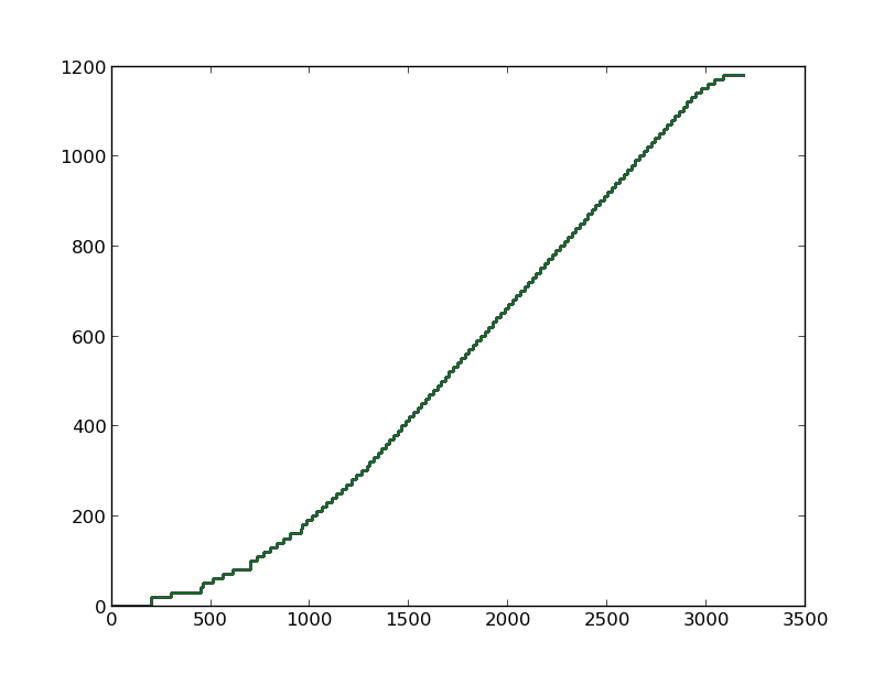
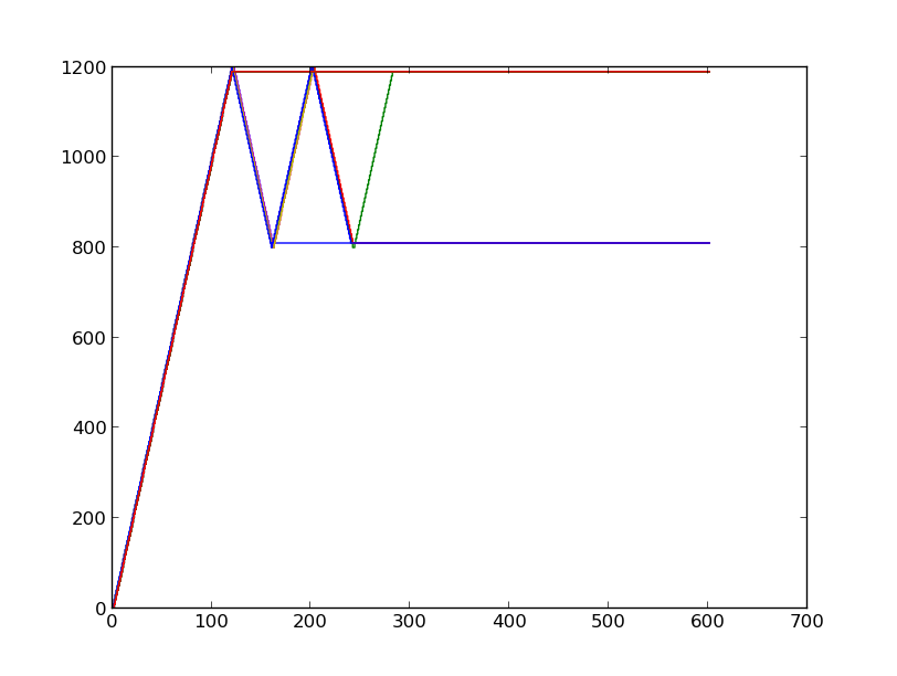
Figure 5: Evolution of the PI-controller: fickle (left) and discrete (right) versions.

The second example is a model for a double integrator, an extension of the simple integrator of Fig. 1 to a system with two interdependent variables $x_{1}$ and $x_{2}$. The system has two components, $P_{1},P_{2}$, where $P_{i}$ is in charge of the evolution of $x_{i}$, for $i\in\{1,2\}$, and each $x_{i}$ is governed by the relation $\dot{x_{i}}=f_{i}(x_{1},x_{2})$. The components $P_{1}$ and $P_{2}$ are concurrent and interact with each other by sending an event when the value of $x_{i}$ changes. Therefore the system mixes message passing and hybrid evolution. This system can be used to solve second order linear differential equations of the form $\ddot{y}=k_{P}\dot{y}+k_{I}(S-y)$; we simply take $\dot{x_{1}}=x_{2}$ and $\dot{x_{2}}=k_{P}x_{2}+k_{I}(S-x_{1})$. This family of equations often appears in control-loop feedback mechanisms, where they model the behavior of proportional-integral (PI) controller. For example, a system with double quantized integrators is studied in [13] in the context of a dynamic cruise controller.

We compare the results obtained with our two versions of the integrator: fickle and discrete (synchronous). Figure. 5 displays the evolution of the variable $x_{1}$ in the PI-controller for our two models, with a quantum of $\nicefrac{{1}}{{10}}$. We observe that the discrete version does not converge with this time step (we need to choose a value of $\nicefrac{{1}}{{100}}$).

System	Landing Gear		Cruise Control (PI-controller)
(version) parameters	(fickle) $Q=\nicefrac{{1}}{{10}}$	(discrete) $h=\nicefrac{{1}}{{10}}$	(fickle) $Q=\nicefrac{{1}}{{10}}$	(discrete) $h=\nicefrac{{1}}{{10}}$	(discrete) $h=\nicefrac{{1}}{{100}}$
# states	1 906	2 590	259	2 049	20 549
time (s)	0.076	0.125	0.004	0.017	0.185
memory (MB)	1.00	1.56	0.11	0.90	9.02

5 Conclusion and Related Work

We have shown how to extend the $SCG$ construction to handle fickle transitions. The $SCG$ is certainly the most widely used state space abstraction for Time Petri nets: it is a convenient abstraction for LTL model checking; it is finite when the set of markings is bounded; and it preserves both the markings and traces of the net. The results are slightly different with dynamic TPN, even for the restricted class of translation nets. In particular, we may have an infinite $SCG$ even when the net is bounded. This may be the case, for instance, if we have a transition that can stay persistent infinitely and that is associated to the fickle function $\textbf{I}_{d}(\theta)=[\theta+1,\theta+1]$. This entails that our construction may not terminate, even if the set of markings is bounded. This situation is quite comparable to what occurs with updatable timed automata [9] and, like in this model, it is possible to prove that the model-checking problem is undecidable in the general case. This does not mean that our construction is useless in practice, as we show in our examples of Sect. 4.

The notion of fickle transitions came naturally as the simplest extension of TPN able to integrate the Quantized State System (QSS) method [10] inside Tina. Although there are still problems left unanswered, this could provide a solution for supporting hybrid systems inside a real-time model-checker. Theorem 2 gives clues on how to support fickle transitions in existing tools for standard TPN. Indeed, the incremental computation of the coefficients of the “difference-bound matrices” ($\alpha,\beta$ and $\gamma$) is not very different from what is already implemented in tools that can generate a $SCG$ for a standard TPN. In particular, the “intermediate” domain $D_{\mathit{int}}$ computed in (C1) is exactly the domain obtained from $D$ in a standard TPN. We only need two added elements. First, we need to apply a numerical function over the coefficients of $D_{\mathit{int}}$; this is easy if the tool already supports associating a function to a transition in a TPN (as it is the case with Tina). Next, we need to compute the maximal value of a numerical functions over a given interval; this can be easily added to the tool or delegated to a numerical solver. Actually, for the examples presented in Sect. 4, we only need to use affine functions, for which the maximal value can be defined by a straightforward arithmetical expression. As a result, it should be relatively easy to adapt existing tools to support the addition of fickle transitions. This assessment is supported by our experience when extending Tina; once the semantics of fickle transitions was stable, it took less than a week to adapt our tools and to obtain the first results.

To our knowledge, updatable TA is the closest model to dynamic TPN. The relation between these two models is not straightforward. We consider very general update functions but do not allow the use of multiple firing dates in an update (that would be the equivalent of using other clocks in TA). Also, the notion of persistent transitions does not exist in TA while it is central in our approach. While the work on updatable TA is geared toward decidability issues, we rather concentrate on the implementation of our extension and its possible applications. Nonetheless, it would be interesting to define a formal, structural translations between the two models, like it was done in [2, 6] between TA and TPN. Some of our results also show similarities between fickle transitions and the use of stopwatch [4]. In the general case, it does not seem possible to encode one extension with the other, but it would be interesting to look further into this question. Finally, since the notion of slope is central in our implementation of the QSS method (see Sect. 2.3), it would be interesting to compare our results with an approach based on multirate transitions [12], that is a model where time does not advance at the same rate in all the transitions.

For future works, we plan to study an extension of our approach to other models of real-time systems and to other state-space abstractions. For instance the Strong $SCG$ construction of [1], that is finer than the $SCG$ construction but that is needed when considering the addition of priorities. The strong $SCG$ relies on the use of clock domains, rather than firing domains, and has some strong resemblance with the zone constructions commonly used for analysis of TA. Another, quite different, type of abstractions rely on the use of a discrete time semantics for TPN. We can obtain a discrete semantic by, for instance, restricting continuous transitions $\mathbin{\smash{\overset{{\theta}}{{\to}}}}$ to the case where $\theta$ is an integer. This approach could be useful when modeling hybrid systems, since it is a simple way to add a quantization over time as well as over values.

Appendix A Proof of Theorem 1

Theorem 1: For every weak DTPN, $N$, with a finite set of reachable markings, there is a TPN, $N^{\times}$, with an equivalent semantics.

We say that two nets have equivalent semantics if their state graphs are weakly timed bisimilar (see Def. 4 below).

We assume that $N$ is the weak DTPN $\langle{P},{T},{\mathbf{Pre}},{\mathbf{Post}},m_{0},\textbf{I}_{s},\textbf{I}_{d}\rangle$. Since $N$ is weak, the function $\textbf{I}_{d}$ is trivial and the behavior of persistent transitions is the same than for TPN. By hypothesis, we also have that the set of markings of $N$, say ${\cal M}$, is bounded.

We define a 1-safe TPN $N^{\times}$ that will simulate the execution of $N$. Some places of $N^{\times}$ will be used to denote the marking in the net $N$. We denote $P_{{\cal M}}$ the set containing one place for every marking in ${\cal M}$. We use the same symbol, $m$, to denote the place and the marking. The places of $P_{{\cal M}}$ are a subset of the places of $N^{\times}$.

Since a TPN is also an example of weak DTPN, our construction can be used in order to find a 1-safe TPN equivalent to any given (bounded) TPN.

Corollary 1.

For every TPN, with a finite set of reachable markings, there is a 1-safe TPN with an equivalent semantics.

The definition of $N^{\times}$ is based on the composition of a collection of TPN, denoted $E(t,I)$, that models the situation where the transition $t$ of $N$ is currently enabled and where the firing date of $t$ was picked in the time interval $I$. Therefore $I$ belongs to the set of time intervals, denoted $\mathbb{I}_{{\cal M}}$, that can appear during the evolution of $N$. The set $\mathbb{I}_{{\cal M}}$ is also finite and has less than $|T|.|{\cal M}|$ elements.

$$\mathbb{I}_{{\cal M}}=\left\{\ \textbf{I}_{s}(k,m)\leavevmode\nobreak\ |\leavevmode\nobreak\ m\in{\cal M},k\in T\ \right\}$$

When dealing with a particular transition $t$, we can restrict to time intervals of the form $\textbf{I}_{s}(t,m)$ where $t$ is enabled at $m$.

$$\mathbb{I}(t)=\left\{\ \textbf{I}_{s}(t,m)\leavevmode\nobreak\ |\leavevmode\nobreak\ t\in{\cal E}(m)\ \right\}$$

Before defining formally $N^{\times}$, we start by defining some useful notations and by giving some intuitions on our encoding.

A.1 Definitions and Useful Notations

We define the TPN $E(t,I)$ for every pair $(t,I)$ of a transition $t$ in $T$ and a time interval $I$ in $\mathbb{I}(t)$. We give a graphical description of the net in Fig. 6.

The net $E(t,I)$ has two places $p_{{t},{I}}$ and $q_{{t},{I}}$. The place $p_{{t},{I}}$ is the initial place of $E(t,I)$. Intuitively, we will place a token in $p_{{t},{I}}$ when the transition $t$ becomes newly-enabled by a marking, say $m$, and $I=\textbf{I}_{s}(t,m)$. The token moves to $q_{{t},{I}}$ when the transition has been enabled for long enough, that is when we reach the firing date of $t$. Hence the purpose of transition $t_{I}$ is to record the timing constraint associated to $t$. This transition is “local” to $E(t,I)$, meaning that no other places in $N^{\times}$ has access to it.

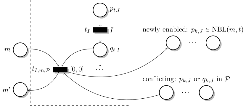
Figure 6: The TPN $E(t,I)$

The final ingredient in the definition of $E(t,I)$ is a collection of transitions $t_{I,m,{\cal P}}$, where the marking $m$ enables $t$, that is $t$ is in ${\cal E}(m)$. These transitions have timing constraints $[0,0]$ and can empty the token in place $q_{{t},{I}}$. The purpose of the transition $t_{I,m,{\cal P}}$ is to model the firing of transition $t$ from the marking $m$ in $N$. In particular, a transition $t_{I,m,{\cal P}}$ will empty the place $m$ of $P_{{\cal M}}$ and put a token in the place $m^{\prime}$ such that $m\mathbin{\smash{\overset{{t}}{{\to}}}}m^{\prime}$, that is $m^{\prime}=m-\mathbf{Pre}(t)+\mathbf{Post}(t)$.

When the transition $t_{I,m,{\cal P}}$ fires, it should also “enable” new transitions and “disable” the transitions that are in conflict with $t$ in $N$. More precisely, the transition should: (1) put a token on the initial place of the net $E(k,J)$, where $k\in\operatorname{nbl}(m,t)$ and $J=\textbf{I}_{s}(k,m^{\prime})$; and (2) remove the token from the net $E(k^{\prime},J^{\prime})$ such that $k^{\prime}$ was enabled at $m$ but not at $m^{\prime}$ (conflicting transitions). The transitions of $N$ that are persistent when $t$ fires are not involved; therefore their firing date are left untouched. The treatment of conflicting transitions is quite complex. Indeed, it is not possible to know exactly the time interval $J^{\prime}$ associated to $k^{\prime}$ and therefore we should test all possible combinations. Another source of complexity is that the token in $E(k^{\prime},J^{\prime})$ can be either in the initial place, $p_{{k^{\prime}},{J^{\prime}}}$, or in the place $q_{{k^{\prime}},{J^{\prime}}}$ (The parameter ${\cal P}$ is used to differentiate the multiple choices.)

We define the predicate $\operatorname{NBL}(m,t)$ that describes the set of initial places of the nets $E(k,J)$ such that $k$ is newly-enabled after $t$ fires from $m$.

$$\operatorname{NBL}(m,t)=\left\{p_{{k},{J}}\leavevmode\nobreak\ |\leavevmode\nobreak\ k\in\operatorname{nbl}(m,t)\wedge\left(m\mathbin{\smash{\overset{{t}}{{\to}}}}m^{\prime}\right)\wedge\left(J=\textbf{I}_{s}(k,m^{\prime})\right)\right\}$$

Likewise, we define the predicate $\operatorname{CFL}(t,m)$ that describes sets of places in the net $E(k,J)$ such that $k$ conflicts with $t$ at marking $m$. The definition of $\operatorname{CFL}$ relies on the relation $t\operatorname{\Join}_{m}k$, meaning that $k$ and $t$ are in conflict in the marking $m$, that is $m\not\geq\mathbf{Pre}(t)+\mathbf{Pre}(k)$. A set of places ${\cal P}$ is in $\operatorname{CFL}(t,m)$ if it has exactly one place in each transition in conflict with $t$.

$$\begin{array}[c]{rcl}\operatorname{\Join}(m,t)&=&\{k\leavevmode\nobreak\ |\leavevmode\nobreak\ m\not\geq\mathbf{Pre}(t)+\mathbf{Pre}(k)\}\\[10.00002pt] \operatorname{CFL}(m,t)&=&\begin{array}[t]{cl}\{\{r_{k_{1},J_{1}},\dots,r_{k_{n},J_{n}}\}\leavevmode\nobreak\ |\nobreak\leavevmode&r\in\{p,q\}\ \wedge\ \operatorname{\Join}(m,t)=\{k_{1},\dots,k_{n}\}\\ &\wedge\ J_{1}\in\mathbb{I}(k_{1})\wedge\dots\wedge J_{n}\in\mathbb{I}(k_{n})\}\\ \end{array}\end{array}$$

There are at most $2^{|T|}$ sets in $\operatorname{CFL}(m,t)$. Next, we use all these predicates to formally define the net $E(t,I)$ and, ultimately, the TPN $N^{\times}$.

Definition 2.

The net $E(t,I)$ is the 1-safe TPN such that:

• the set of places is $P^{\times}$;

  $$P^{\times}=P_{{\cal M}}\cup\{p_{{t},{I}},q_{{t},{I}}\leavevmode\nobreak\ |\leavevmode\nobreak\ t\in T,I\in\mathbb{I}(t)\}$$

• the set of transitions is $\{t_{I}\}\cup\{t_{I,m,{\cal P}}\leavevmode\nobreak\ |\leavevmode\nobreak\ t\in{\cal E}(m),{\cal P}\in\operatorname{CFL}(m,t)\}$;

• the pre- and postconditions of $t_{I}$ are as in Fig. 6;

• the places in the precondition of $t_{I,m,{\cal P}}$ are $\{q_{{t},{I}},m\}\cup{\cal P}$

• the places in the postcondition of $t_{I,m,{\cal P}}$ are $\{m^{\prime}\}\cup\operatorname{NBL}(m,t)$

• the static time interval of $t_{I}$ is $I$ and of the transitions $t_{I,m,{\cal P}}$ is $[0,0]$;

• there is no token in the net in the initial marking;

All the nets $E(t,I)$ have the same set of places. The net $N^{\times}$ is the 1-safe TPN obtained by the “union” of the nets $E(t,I)$; places with the same identifier are fusioned and transitions are not composed.

Definition 3.

The net $N^{\times}$ is the 1-safe TPN such that:

• the set of places is $P^{\times}$, as in Def. 2;

• the set of transitions is $T^{\times}$;

  $$T^{\times}=\{t_{I},t_{I,m,{\cal P}}\leavevmode\nobreak\ |\leavevmode\nobreak\ m\in{\cal M},t\in{\cal E}(m),I\in\mathbb{I}(t),{\cal P}\in\operatorname{CFL}(m,t)\}$$

• the static time interval and the pre- and postconditions of the transitions in $T^{\times}$ are as in Def. 2;

• in the initial marking there is one token in each place $p_{{t},{I}}$ such that $t$ is enabled at $m_{0}$, the initial marking of $N$, and $I=\textbf{I}_{s}(t,m_{0})$;

Our encoding of $N$ is not very concise. Indeed, the best bounds for the size of $N^{\times}$ are in $O(|T|.|{\cal M}|)$ for the number of places and in $O(2^{|T|}.|T|.|{\cal M}|^{2})$ for the number of transitions. We can strengthen these bounds if $N$ is a TPN, that is when there is only one possible time interval for each transition. In this case the bound for the number of places is $O(|T|+|{\cal M}|)$ and the bound for the number of transitions is in $O(|T|.2^{|T|})$. We can also choose a more concise representation for the markings; such that we use a vector of places to encode the possible markings (in binary format) instead of using one place for every single marking (a representation in unary format).

A.2 Correctness of our Encoding

We start by recalling the notion of (weak) timed similarity between Timed Transition Systems (TTS) (see for example [The Expressive Power of Time Petri Nets, Bérard et al, 2012]). We consider a distinguished set of actions that stands for “silent/unobservable events”; we assume that every silent action as the label $\tau$. The weak transition relation $\mathbin{\smash{\overset{{\alpha}}{{\Rightarrow}}}}$ is defined as $\left(\mathbin{\smash{\overset{{\tau}}{{\to}}}}\right)^{*}\mathbin{\smash{\overset{{\alpha}}{{\to}}}}$ if $\alpha\neq\tau$ and as $\left(\mathbin{\smash{\overset{{\tau}}{{\to}}}}\right)^{*}$ otherwise. Hence we always have $s\mathbin{\smash{\overset{{\tau}}{{\Rightarrow}}}}s$ for every state $s$.

Definition 4.

Assume $SG_{1}=\langle S_{1},S^{1}_{0},\rightarrow_{1}\rangle$ and $SG_{2}=\langle S_{2},S^{2}_{0},\rightarrow_{2}\rangle$ are two TTS. A binary relation ${\cal R}$ over $S_{1}\times S_{2}$ is a weak timed simulation if, whenever $s_{1}\mathbin{\smash{\overset{{\alpha}}{{\to}}_{1}}}s^{\prime}_{1}$ in $SG_{1}$ then for every state $s_{2}\in S_{2}$ such that $s_{1}{\cal R}s_{2}$ there is a state $s^{\prime}_{2}$ such that $s_{2}\mathbin{\smash{\overset{{\alpha}}{{\Rightarrow}}_{2}}}s^{\prime}_{2}$ and $s^{\prime}_{1}{\cal R}s^{\prime}_{2}$.

We say that two TTS are (weakly timed) bisimilar, denoted $SG_{1}\approx SG_{2}$, if there is a binary relation ${\cal R}$ over $S_{1}\times S_{2}$ such that both ${\cal R}$ and ${\cal R}^{-1}$ are weak timed simulations.

Next we show that $SG$, the state graph of $N$, and $SG^{\times}$, the state graph of $N^{\times}$, are bisimilar. The definition of $\approx$ depends implicitly on the definition of the silent events $\tau$. In our case, the only silent actions correspond to the discrete events $t_{I}$ in $T^{\times}$. Intuitively, an action of the form $t_{I}$ only indicates that the transition $t\in T$ has reached its firing date. It has no effect on the marking (places in $P_{{\cal M}}$) or on the other nets $E(k,J)$. On the opposite, an action $t_{I,m,{\cal P}}$ commits the decision to fire $t$. We use the action $t$ to refer to any transition of the kind $t_{I,m,{\cal P}}$ in $SG^{\times}$.

We list a sequence of properties on the semantics of $N^{\times}$. Since this a 1-safe net, we say that a place $r$ is marked on a state $(m^{\times},\varphi^{\times})$ of $N^{\times}$ if $m^{\times}(r)=1$. The following properties hold on every reachable state in $SG^{\times}$:

1. there is only one token marked in the places $P_{{\cal M}}$;

2. if $m$ is marked then there is only one token among the collection of (sub)nets $E(t,I)$, for every $t\in{\cal E}(m)$. Moreover there are no token in the net $E(k,J)$ if $k\notin{\cal E}(m)$;

3. if the places $m$ and $q_{{t},{I}}$ of $E(t,I)$ are marked then there is exactly one set ${\cal P}$ in $\operatorname{CFL}(m,t)$ such that $t_{I,m,{\cal P}}$ is enabled; this is the only transition enabled in $E(t,I)$.

We can prove these properties by induction on the sequence of transitions (the path) from the initial state of $SG^{\times}$ to a state. If the net $E(t,I)$ is marked, it means that the timing constraints of $t$, at the time it was newly enabled, was $I$.

We define an interpretation function ${[\![}\,{.}\,{]\!]}$ between states of $SG^{\times}$ and states of $SG$. Assume $s_{\times}=(m^{\times},\varphi^{\times})$ is a state in $SG^{\times}$, then ${[\![}\,{s_{\times}}\,{]\!]}$ is the state $(m,\varphi)$ such that:

• the marking $m$ corresponds to the only place of the kind $m\in P_{{\cal M}}$ that is marked in $m^{\times}$ (see property 1 above);

• for every $t\in{\cal E}(m)$ there is a unique net $E(t,J)$ marked in $N^{\times}$ (see property 2 above), then if the place $p_{{t},{J}}$ is marked we have $\varphi(t)=\varphi^{\times}(t_{t,J})$ and if $q_{{t},{J}}$ is marked we have $\varphi(t)=0$.

We observe that, with our interpretation, the initial states of $SG^{\times}$ is mapped to the initial state of $SG$. Again, using an induction on the paths of $SG^{\times}$, it is possible to prove that every state of the form ${[\![}\,{s_{\times}}\,{]\!]}$ is reachable in $N$. Conversely, we prove that every state in $SG$ has a counterpart in $SG^{\times}$. Actually, we prove a stronger property that will be useful to prove the equivalence between state graphs.

Lemma 1.

For every state $s\in SG$ there is a state $s_{\times}\in SG^{\times}$ such that $s={[\![}\,{s_{\times}}\,{]\!]}$ and for every action $\alpha\in T\cup\mathbb{R}_{\geq 0}$; if $s\mathbin{\smash{\overset{{\alpha}}{{\to}}}}s^{\prime}$ then there is a state ${s^{\prime}_{\times}}$ in $SG^{\times}$ such that ${s_{\times}}\mathbin{\smash{\overset{{\alpha}}{{\Rightarrow}}}}{s^{\prime}_{\times}}$ and $s^{\prime}={[\![}\,{s^{\prime}_{\times}}\,{]\!]}$.

sketch.

By induction on the sequence of transitions from the initial state $s_{0}$ of $SG$ to $s$. We already observed that $s_{0}$ is the interpretation of the initial state of $SG^{\times}$. Assume that $s=(m,\varphi)$ has a counterpart $s_{\times}$ in $SG^{\times}$ and that $s\mathbin{\smash{\overset{{\alpha}}{{\to}}}}s^{\prime}$.

We first study the case of discrete transitions, that is $\alpha=t$ with $t\in{\cal E}(m)$. Assume $E(t,I)$ is the net marked in $s_{\times}$ that corresponds to $t$. Since there is a discrete transition from $s$, we have that $\varphi(t)=0$, which means that either $tI^{\times}(t_{I})=0$ (the transition can fire in $N^{\times}$) or that $q_{{t},{I}}$ is already marked. Then there is a unique set ${\cal P}$ such that $t_{I,m,{\cal P}}$ can fire, and it can fire immediately. This means that there is a state $s^{\prime}_{\times}$ such that $s_{\times}\mathbin{\smash{\overset{{t}}{{\Rightarrow}}}}s^{\prime}_{\times}$. By definition of $t_{I,m,{\cal P}}$, we can choose the same firing dates for the newly enabled transitions in $s^{\prime}_{\times}$ than in $s^{\prime}$, hence $s^{\prime}={[\![}\,{s^{\prime}_{\times}}\,{]\!]}$.

Assume that $\alpha$ is a continuous action $\theta\in\mathbb{R}_{\geq 0}$. We need to prove that we can let the time elapse of $\theta$ in the state $SG^{\times}$. We can assume that $\theta\neq 0$, otherwise $s^{\prime}=s$. Since we can let $\theta$ elapse from $s$ we have that $\theta\leq\varphi(t)$ for every transition $t\in{\cal E}(m)$. By definition of ${[\![}\,{.}\,{]\!]}$ we have that $\varphi(t)=\varphi^{\times}(t_{I})$ for some interval $I\in\mathbb{I}(t)$. Then we also have ${s_{\times}}\mathbin{\smash{\overset{{\theta}}{{\Rightarrow}}}}{s^{\prime}_{\times}}$ and $s^{\prime}={[\![}\,{s^{\prime}_{\times}}\,{]\!]}$. ∎

Our candidate relation ${\cal R}$ for the bisimulation is the binary relation from $SG\times SG^{\times}$ such that $s\mathrel{{\cal R}}s^{\times}$ if and only if $s={[\![}\,{s^{\times}}\,{]\!]}$. From our previous results we already have that ${\cal R}$ is total. Hence we just need to prove that both ${\cal R}$ and ${\cal R}^{-1}$ are simulations. The property for ${\cal R}$ is a direct corollary of Lemma 1. For the inverse relation, we assume that $s_{\times}\mathbin{\smash{\overset{{\alpha}}{{\to}}}}s^{\prime}_{\times}$ in $SG^{\times}$. We have three possible case for the action $\alpha$. The case $\alpha=\tau$ is trivial since, in this case, we have ${[\![}\,{s_{\times}}\,{]\!]}={[\![}\,{s^{\prime}_{\times}}\,{]\!]}$. The cases where $\alpha$ is a discrete transition $t$ or a continuous transition $\alpha\in\mathbb{R}_{\geq 0}$ is similar than for Lemma 1. Hence $SG$ and $SG^{\times}$ are weakly time bisimilar. QED.

References

- [1] B. Berthomieu and F. Vernadat. State class constructions for branching analysis of Time Petri Nets. In TACAS2003, volume LNCS2619, page 442. Springer, 2003.
- [2] B. Bérard and F. Cassez. Comparison of the expressiveness of timed automata and time petri nets. In Proc. FORMATS’05, vol. 3829 of LNCS, pages 211–225. Springer, 2005.
- [3] B. Berthomieu and M. Diaz. Modeling and verification of time dependent systems using time Petri nets. IEEE Trans. on Software Engineering, 17(3):259–273, 1991.
- [4] B. Berthomieu, D. Lime, O.H. Roux, and F. Vernadat. Reachability problems and abstract state spaces for time Petri nets with stopwatches. Journal of Discrete Event Dynamic Systems, 17:133-158, 2007.
- [5] B. Berthomieu and M. Menasche. A state enumeration approach for analyzing time Petri nets. In Proc. Applications and Theory of Petri Nets (ATPN’82), pages 27–56, 1982.
- [6] B. Berthomieu, F. Peres, and F. Vernadat. Bridging the gap between timed automata and bounded time petri nets. In Formal Modeling and Analysis of Timed Systems (FORMATS’06), Springer LNCS 4202, pages 82–97, 2006.
- [7] B. Berthomieu, P.-O. Ribet, and F. Vernadat. The tool TINA – construction of abstract state spaces for Petri nets and time Petri nets. International Journal of Production Research, 42(14):2741–2756, 15 July 2004.
- [8] Frédéric Boniol and Virginie Wiels. The Landing Gear System Case Study. In ABZ Case Study, volume 433 of Communications in Computer Information Science. Springer, 2014.
- [9] Patricia Bouyer, Catherine Dufourd, Emmanuel Fleury, and Antoine Petit. Updatable timed automata. Theoretical Computer Science, 321(2–3):291–345, 2004.
- [10] Francois E. Cellier and Ernesto Kofman. Continuous System Simulation. Springer, 2006.
- [11] François E Cellier, Ernesto Kofman, Gustavo Migoni, and Mario Bortolotto. Quantized state system simulation. Proc. GCMS’08, Grand Challenges in Modeling and Simulation, pages 504–510, 2008.
- [12] C. Daws and S. Yovine. Two examples of verification of multirate timed automata with kronos. In Proc. 1995 IEEE Real-Time Systems Symposium, RTSS’95, pages 66–75. IEEE Computer Society Press, 1995.
- [13] Damien Foures, Vincent Albert, and Alexandre Nketsa. Formal compatibility of experimental frame concept and FD-DEVS model. Proc. of MOSIM’12, International Conference of Modeling, Optimization and Simulation, 2012.
- [14] Guillaume Gardey, Didier Lime, Morgan Magnin, and Olivier H Roux. Romeo: a tool for analyzing time petri nets. In Proceedings of the 17th international conference on Computer Aided Verification, pages 418–423. Springer, 2005.
- [15] P. M. Merlin. A study of the recoverability of computing systems. PhD thesis, Department of Information and Computer Science, University of California, 1974.
- [16] Odile Nasr, Miloud Rached, Jean-Paul Bodeveix, and Mamoun Filali. Spécification et vérification d’un ordonnanceur en B via les automates temporisés. L’Objet, 14(4), 2008.
- [17] G. Ramalingam, J. Song, L. Joscovicz, and R. E. Miller. Solving difference constraints incrementally. Algorithmica, 23, 1995.
- [18] Enrico Vicario, Luigi Sassoli, and Laura Carnevali. Using stochastic state classes in quantitative evaluation of dense-time reactive systems. IEEE Trans. Software Eng., 35(5):703–719, 2009.