Probably Approximately Correct MDP Learning and Control With Temporal Logic Constraints

Abstract

We consider synthesis of control policies that maximize the probability of satisfying given temporal logic specifications in unknown, stochastic environments. We model the interaction between the system and its environment as a Markov decision process (MDP) with initially unknown transition probabilities. The solution we develop builds on the so-called model-based probably approximately correct Markov decision process (PAC-MDP) methodology. The algorithm attains an $\varepsilon$-approximately optimal policy with probability $1-\delta$ using samples (i.e. observations), time and space that grow polynomially with the size of the MDP, the size of the automaton expressing the temporal logic specification, $\frac{1}{\varepsilon}$, $\frac{1}{\delta}$ and a finite time horizon. In this approach, the system maintains a model of the initially unknown MDP, and constructs a product MDP based on its learned model and the specification automaton that expresses the temporal logic constraints. During execution, the policy is iteratively updated using observation of the transitions taken by the system. The iteration terminates in finitely many steps. With high probability, the resulting policy is such that, for any state, the difference between the probability of satisfying the specification under this policy and the optimal one is within a predefined bound.

I Introduction

Integrating model-based learning into control allows an agent to complete its assigned mission by exploring its unknown environment, using the gained knowledge to gradually approach an (approximately) optimal policy. In this approach, learning and control complement each other. For the controller to be effective, there is a need for correct and sufficient knowledge of the system. Meanwhile, by exercising a control policy, the agent obtains new percepts, which is then used in learning to improve its model of the system. In this paper, we propose a method that extends model-based probably approximately correct Markov decision process (PAC-MDP) reinforcement learning to temporal logic constrained control for unknown, stochastic systems.

A stochastic system with incomplete knowledge can be modeled as an MDP in which the transition probabilities are unknown. Take a robotic motion planning problem as an example. Different terrains where the robot operates affect its dynamics in a way that, for the same action of the robot, the probability distributions over the arrived positions differ depending on the level and coarseness of different grounds. The robot dynamics in an unknown terrain can be modeled as an MDP in which the transition probabilities are unknown. Acquiring such knowledge through observations of robot’s movement requires large, possibly infinite number of samples, which is neither realizable nor affordable in practice. Alternatively, with finite amount of samples, we may be able to approximate the actual MDP and reason about the optimality and correctness (w.r.t. the underlying temporal logic specifications) of policies synthesized using this approximation.

The thesis of this paper is to develop an algorithm that computational efficiently updates the controller subject to temporal logic constraints for an unknown MDP. We extend the PAC-MDP method [1, 2] to maximize the probability of satisfying a given temporal logic specification in an MDP with unknown transition probabilities. In the proposed method, the agent maintains a model of the MDP learned from observations (transitions between different states enabled by actions) and when the learning terminates, the learned MDP approximates the true MDP to a specified degree, with a pre-defined high probability. The algorithm balances exploration and exploitation implicitly: Before the learning stops, either the current policy is approximately optimal, or new information can be invoked by exercising this policy. Finally, at convergence, the policy is ensured to be approximately optimal, and the time, space, and sample complexity of achieving this policy is polynomial in the size of the MDP, in the size of the automaton expressing the temporal logic specification and other quantities that measure the accuracy of, and the confidence in, the learned MDP with respect to the true one.

Existing results in temporal logic constrained verification and control synthesis with unknown systems are mainly in two categories: The first uses statistical model checking and hypothesis testing for Markov chains [3] and MDPs [4]. The second applies inference algorithms to identify the unknown factors and adapt the controller with the inferred model (a probabilistic automaton, or a two-player deterministic game) of the system and its environment [5, 6]. Statistical model checking for MDPs [4] relies on sampling of the trajectories of Markov chains induced from the underlying MDP and policies to verify whether the probability of satisfying a bounded linear temporal logic constraint is greater than some quantity for all admissible policies. It is restricted to bounded linear temporal logic properties in order to make the sampling and checking for paths computationally feasible. For linear temporal logic specifications in general, computationally efficient algorithm has not been developed. Reference [7] employs inference algorithms for deterministic probabilistic finite-state automata to identify a subclass of MDPs, namely, deterministic MDPs. Yet, this method requires the data (the state-action sequences in the MDPs) to be independent and identically distributed. Such an assumption cannot hold in the paradigm where learning (exploration) and policy update (exploitation) are carried out in parallel and at run time, simply because that the controller/policy introduces sampling bias for observations of the system. Reference [5] applies stochastic automata learning combined with probabilistic model checking for stochastic systems. However, it requires an infinite amount of experiences for the model to be identified and the policy to be optimal, and may not be affordable in practice.

We show that the extension of the PAC-MDP method to control synthesis subject to temporal logic constraints shares many attractive features with the original method: First, it applies to linear temporal logic specifications and guarantees efficient convergence to an approximately optimal policy within a finite time horizon and the number of policy updates is determined by the size of underlying MDP, independent from the specification. Second, it balances the exploration (for improving the knowledge of the model) and exploitation (for maximizing the probability of satisfying the specification) and does not require the samples to be independent and identically distributed.

II Preliminaries

Definition 1.

A labeled MDP is a tuple $M=\langle Q,\Sigma,q_{0},P,\mathcal{AP},L\rangle$ where $Q$ and $\Sigma$ are finite state and action sets. $q_{0}\in Q$ is the initial state. The transition probability function $P:Q\times\Sigma\times Q\rightarrow[0,1]$ is defined such that $\sum_{q^{\prime}\in Q}P(q,\sigma,q^{\prime})\in\{0,1\}$ for any state $q\in Q$ and any action $\sigma\in\Sigma$. $\mathcal{AP}$ is a finite set of atomic propositions and $L:Q\rightarrow 2^{\mathcal{AP}}$ is a labeling function which assigns to each state $q\in Q$ a set of atomic propositions $L(q)\subseteq\mathcal{AP}$ that are valid at the state $q$. $L$ can be extended to state sequences in the usual way, i.e., $L(\rho_{1}\rho_{2})=L(\rho_{1})L(\rho_{2})$ for $\rho_{1},\rho_{2}\in Q^{\ast}$.

The structure of the labeled MDP $M$ is the underlying graph $\langle Q,\Sigma,E\rangle$ where $E\subseteq Q\times\Sigma\times Q$ is the set of labeled edges. $(q,\sigma,q^{\prime})\in E$ if and only if $P(q,\sigma,q^{\prime})\neq 0$. We say action $\sigma$ is enabled at $q$ if and only if there exists $q^{\prime}\in Q$, $(q,\sigma,q^{\prime})\in E$.

A deterministic policy $f:Q^{\ast}\rightarrow\Sigma$ is such that given $\rho=q_{0}\ldots q_{n}$, $f(\rho)=\sigma$ only if $\sigma$ is enabled at $q_{n}$.

II-A A specification language

We consider to use linear temporal logic formula (LTL) to specify a set of desired system properties such as safety, liveness, persistence and stability. A formula in LTL is built from a finite set of atomic propositions $\mathcal{AP}$, $\mathsf{true}$, $\mathsf{false}$ and the Boolean and temporal connectives $\land,\lor,\neg,\Rightarrow,\Leftrightarrow$ and $\square$ (always), $\mathcal{U}$ (until), $\lozenge$ (eventually), $\bigcirc$ (next). Given a LTL formula $\varphi$ as the system specification, one can always represent it by a deterministic Rabin automaton (DRA) $\mathcal{A}_{\varphi}=\langle S,2^{\mathcal{AP}},T_{s},I_{s},\mathsf{Acc}\rangle$ where $S$ is a finite state set, $2^{\mathcal{AP}}$ is the alphabet, $I_{s}\in S$ is the initial state, and $T_{s}:S\times 2^{\mathcal{AP}}\rightarrow S$ the transition function. The acceptance condition $\mathsf{Acc}$ is a set of tuples $\{(J_{i},K_{i})\mid i=0,1,\ldots,m\}$ consisting of subsets $J_{i}$ and $K_{i}$ of $S$. The run for an infinite word $w=w[0]w[1]\ldots\in(2^{\mathcal{AP}})^{\omega}$ is the infinite sequence of states $s_{0}s_{1}\ldots\in S^{\omega}$ where $s_{0}=I_{s}$ and $s_{i+1}=T_{s}(s_{i},w[i])$. A run $\rho=s_{0}s_{1}\ldots$ is accepted in $\mathcal{A}_{\varphi}$ if there exists at least one pair $(J_{i},K_{i})\in\mathsf{Acc}$ such that $\mathsf{Inf}(\rho)\cap J_{i}=\emptyset$ and $\mathsf{Inf}(\rho)\cap K_{i}\neq\emptyset$ where $\mathsf{Inf}(\rho)$ is the set of states that appear infinitely often in $\rho$.

Given an MDP and a LTL specification $\varphi$, we aims to maximize the probability of satisfying $\varphi$ from a given state. Such an objective is quantitative [8].

II-B Policy synthesis in a known MDP

We now present a standard quantitative synthesis method in a known MDP with LTL specifications, following from [9, 8].

Definition 2.

Given an MDP $M=\langle Q,\Sigma,P,q_{0},\mathcal{AP},L\rangle$ and the DRA $\mathcal{A}_{\varphi}=\langle S,2^{\mathcal{AP}},T_{s},I_{s},\{(J_{i},K_{i})\mid i=1,\ldots,m\}\rangle$, the product MDP is $\mathcal{M}=M\ltimes\mathcal{A}_{\varphi}=\langle V,\Sigma,\Delta,v_{0},\mathsf{Acc}\rangle$,
with components defined as follows: $V=Q\times S$ is the set of states. $\Sigma$ is the set of actions. The initial state is $v_{0}=(q_{0},s_{0})$ where $s_{0}=T_{s}(I_{s},L(q_{0}))$. $\Delta:V\times\Sigma\times V\rightarrow[0,1]$ is the transition probability function. Given $v=(q,s)$, $\sigma$, $v^{\prime}=(q^{\prime},s^{\prime})$, let $\Delta(v,\sigma,v^{\prime})=P(q,\sigma,q^{\prime})$ and $T_{s}(s,L(q^{\prime}))=s^{\prime}$. The acceptance condition is $\mathsf{Acc}=\{(\hat{J_{i}},\hat{K_{i}}),i:=1,\ldots,m\mid\hat{J_{i}}=Q\times J_{i},\hat{K_{i}}=Q\times K_{i}\}$, which is obtained by lifting of the set $J_{i},K_{i}\subseteq S$ the acceptance condition of $\mathcal{A}_{\varphi}$ into $\mathcal{M}$.

A memoryless, deterministic policy for a product MDP $\mathcal{M}=\langle V,\Sigma,\Delta,v_{0},\mathsf{Acc}\rangle$ is a function $f:V\rightarrow\Sigma$. A memoryless policy $f$ in $\mathcal{M}$ is in fact a finite-memory policy $f^{\prime}$ in the underlying MDP $M$. Given a state $(q,s)\in V$, we can consider $s$ to be a memory state, and define $f^{\prime}(\rho)=f((q,s))$ where the run $\rho=q_{0}q_{1}\ldots q_{n}$ satisfies $q_{n}=q$ and $T_{s}(I_{s},L(\rho))=s$.

For the types of MDPs, which are one-player stochastic games, memoryless, deterministic policies in the product MDP are sufficient to achieve the quantitative temporal logic objectives [10]. In this work, by policy, we refer to memoryless, deterministic policy. In Section VI, we briefly discuss the extension of PAC-MDP method to two-player stochastic games.

Definition 3 (Markov chain induced by a policy).

Given an MDP $\mathcal{M}=\langle V,\Sigma,\Delta,v_{0},\mathsf{Acc}\rangle$ and a policy $f:V\rightarrow\Sigma$, the Markov chain induced by policy $f$ is a tuple $\mathcal{M}^{f}=\langle V,\Sigma,\Delta^{f},v_{0},\mathsf{Acc}\rangle$ where $\Delta^{f}(v,v^{\prime})=\Delta(v,f(v),v^{\prime})$.

A path in a Markov chain is a (finite or infinite) sequence of states $x\in V^{\ast}$ (or $V^{\omega}$). Given a Markov chain $\mathcal{M}^{f}$, starting from the initial state $v_{0}$, the state visited at the step $t$ is a random variable $X_{t}$. The probability of reaching state $v^{\prime}$ from state $v$ in one step, denoted $\mathrm{Pr}(X_{t+1}=v^{\prime}\mid X_{t}=v)$, equals $\Delta^{f}(v,v^{\prime})$. This is extended to a unique measure $\mathrm{Pr}$ over a set of (infinite) paths of $\mathcal{M}^{f}$, $\mathrm{Pr}(v_{0}v_{1}\ldots v_{n})=\mathrm{Pr}(X_{n}=v_{n}\mid X_{n-1}=v_{n-1})\cdot\mathrm{Pr}(v_{0}v_{1}\ldots v_{n-1})$.

The following notations are used in the rest of the paper: For a Markov chain $\mathcal{M}^{f}$, let $h^{\leq i}(v,X)$ (resp. $h^{i}(v,X)$) be the probability of that a path starts from state $v$ and hits the set $X$ for the first time within $i$ steps (resp. at the exact $i$-th step). By definition, $h^{\leq i}(v,X)=\sum_{k=0}^{i}h^{i}(q,X)$. In addition, let $h(v,X)=\sum_{k=0}^{\infty}h^{k}(v,X)$, which is the probability of a path that starts from state $v$ and enters the set $X$ eventually. When multiple Markov chains are involved, we write $h_{\mathcal{M}^{f}}$ and $\mathrm{Pr}_{\mathcal{M}^{f}}$ to distinguish the hitting probability $h$ and the probability measure $\mathrm{Pr}$ in $\mathcal{M}^{f}$.

Definition 4.

The end component for the product MDP $\mathcal{M}$ denotes a pair $(W,f)$ where $W\subseteq V$ is non-empty and $f:W\rightarrow\Sigma$ is defined such that  for any $v\in W$, $\sum_{v^{\prime}\in W}\Delta(v,f(v),v^{\prime})=1$; and the induced directed graph $(W,\rightarrow_{f})$ is strongly connected. Here, $v\rightarrow_{f}v^{\prime}$ is an edge in the directed graph if $\Delta(v,f(v),v^{\prime})>0$. An accepting end component (AEC) is an end component such that $W\cap\hat{J_{i}}=\emptyset$ and $W\cap\hat{K_{i}}\neq\emptyset$ for some $i\in\{1,\ldots,m\}$.

Let the set of AECs in $\mathcal{M}$ be denoted $\mathsf{AEC}(\mathcal{M})$ and let the set of accepting end states be $\mathcal{C}=\{v\mid\exists(W,f)\in\mathsf{AEC}(\mathcal{M}),v\in W\}$. Due to the property of AECs, once we enter some state $v\in\mathcal{C}$, we can find an AEC $(W,f)$ such that $v\in W$, and initiate the policy $f$ such that for some $i\in\{1,\ldots,m\}$, all states in $\hat{J_{i}}$ will be visited only finite number of times and some state in $\hat{K_{i}}$ will be visited infinitely often. Given the structure of $\mathcal{M}$, the set $\mathsf{AEC}(\mathcal{M})$ can be computed by algorithms in [11, 12]. Therefore, given the system MDP $M$ and its specification automaton $\mathcal{A}_{\varphi}$, to maximize the probability of satisfying the specification, we want to synthesize a policy $f$ that maximizes the probability of hitting the set of accepting end states $\mathcal{C}$, and after hitting the set, a policy in the accepting end component will be followed.

II-C Problem statement

The synthesis method in Section II produces the optimal policy for quantitative temporal logic objectives only if the MDP model is known. However, in practice, such a knowledge of the underlying MDP may not be available. One example can be the robotic motion planning in an unknown terrain.

Model-based reinforcement learning approach suggests the system learns a model of the true MDP on the run, and uses the knowledge to iteratively updates the synthesized policy. Moreover, the learning and policy update shall be efficient and eventually the policy converges to one which meets a certain criterion of success. Tasked with maximizing the probability of satisfying the specification, we define, for a given policy, the state value in the product MDP is the probability satisfying the specification from that state onwards and the optimal policy is the one that maximizes the state value for each individual state in the product MDP. The probability of satisfying a LTL specification is indeed the probability of entering the set of accepting end states in the product MDP (see Section II). We introduce the following definition.

Definition 5.

Let $\mathcal{M}$ be the product MDP, $\mathsf{AEC}(\mathcal{M})$ be the set of accepting end components, and $f$ be a policy in $\mathcal{M}$. For each state $v\in V$, given a finite horizon $T\in\mathbb{N}$, the $T$-step state value is $U^{f}_{\cal M}(v,T)=h^{\leq T}_{\mathcal{M}^{f}}(v,\mathcal{C})$, where $\mathcal{C}$ is the set of accepting end states obtained from $\mathsf{AEC}(\mathcal{M})$. The optimal $T$-step state value is $U_{\cal M}^{\ast}(v,T)=\max_{f}\{U_{\cal M}^{f}(v,T)\}$, and the optimal $T$-step policy is $f^{\ast}_{T}=\arg\max_{f}\{U_{\cal M}^{f}(v,T)\}$. Similarly, We define the state value $U_{\mathcal{M}}^{f}(v)=h_{\mathcal{M}^{f}}(v,\mathcal{C})$. The optimal state value is $U_{\cal M}^{\ast}(v)=\max_{f}\{U_{\cal M}^{f}(v)\}$ and the optimal policy is $f^{\ast}=\arg\max_{f}\{U_{\cal M}^{f}(v)\}$.

The definition of state-value (resp. $T$-step state value) above can also be understood as the following: For a transition from state $v$ to $v^{\prime}$, the reward is $0$ if neither $v$ or $v^{\prime}$ is in $\mathcal{C}$ or if $v\in\mathcal{C}$ and $v^{\prime}\in\mathcal{C}$; the reward is $1$ if $v\notin\mathcal{C}$ and $v^{\prime}\in\mathcal{C}$ and prior to visiting $v$, no state in $\mathcal{C}$ has been visited. Given a state $v$, its state value (resp. $T$-step state value) for a given policy is the expectation on the eventually (resp. $T$ steps) accumulated reward from $v$ under the policy.

We can now state the main problem of the paper.

Problem 1.

Given an MDP $M=\langle Q,\Sigma,q_{0},P,\mathcal{AP},L\rangle$ with unknown transition probability function $P$, and a LTL specification automaton $\mathcal{A}_{\varphi}=\langle S,2^{\mathcal{AP}},T_{s},I_{s},\mathsf{Acc}\rangle$, design an algorithm which with probability at least $1-\delta$, outputs a policy $f:Q\times S\rightarrow\Sigma$ such that for any state $(q,s)$, the $T$-step state value of policy $f$ is $\varepsilon$-close to the optimal state value in $\mathcal{M}$, and the sample, space and time complexity required for this algorithm is less than some polynomial in the relevant quantities $(\left|Q\right|,\left|S\right|,\left|\Sigma\right|,\frac{1}{\varepsilon},T,\frac{1}{\delta})$.

III Main result

III-A Overview

First we provide an overview of our solution to Problem 1. Assume that the system has full observations over the state and action spaces, in the underlying MDP $M$, the set of states are partitioned into known and unknown states (see Definition 8). Informally, a state becomes known if it has been visited sufficiently many times, which is determined by some confidence level $1-\delta$ and a parameter $\epsilon$, the number of states and the number of actions in $M$, and a finite-time horizon $T$.

Since the true MDP is unknown, we maintain and update a learned MDP $\overline{M}$, consequently $\overline{\mathcal{M}}$. Based on the partition of known and unknown states, and the estimations of transition probabilities for the set of known states $H\subseteq Q$, we consider that the set of states $\hat{H}=H\times S$ in $\overline{\mathcal{M}}$ is known and construct a sub-MDP $\overline{\mathcal{M}}_{\hat{H}}$ of $\overline{\mathcal{M}}$ that only includes the set of known states $\hat{H}$, with an additional sink (or absorbing) state that groups together the set of unknown states $V\setminus\hat{H}$. A policy is computed in order to maximize the probability of hitting some target set in $\overline{\mathcal{M}}_{\hat{H}}$ within a finite-time horizon $T$. We show that by following this policy, in $T$ steps, either there is a high probability of hitting a state in the accepting end states of $\mathcal{M}$, or some unknown state will be explored, which at some point will make an unknown state to be known.

Once all states become known, the structure of $M$ must have been identified and the set of accepting end components in the learned product MDP $\overline{\mathcal{M}}$ is exactly these in the true product MDP $\mathcal{M}$. As a result, with probability at least $1-\delta$, the policy obtained in $\overline{\mathcal{M}}$ is near optimal. Informally, a policy $f$ is near optimal, if, from any initial state, the probability of satisfying the specification with $f$ in $T$ steps is no less than the probability of eventually satisfying the specification with the optimal policy, minus a small quantity.

Example

Consider the MDP taken from [9, p.855], as a running example. The objective is to always eventually visiting the state $q_{3}$. That is, $\varphi=\square\lozenge q_{3}$. In [9], the MDP is fully known and the algorithm for computing the optimal policy is given. As the MDP has already encoded the information of the specification, the atomic propositions are omitted and we can use the MDP $M$ as the product MDP $\mathcal{M}$ with acceptance condition $\{(\emptyset,\{q_{3}\})\}$ and the accepting end component is $(\{q_{3}\},f(q_{3})=\alpha)$.

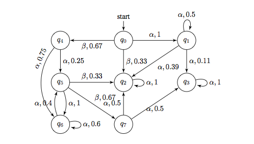
Figure 1: Example of an MDP with states $Q=\{q_{i},i=0,\ldots,7\}$, actions $\Sigma=\{\alpha,\beta\}$, and transition probability function $P$ as indicated.

For this known MDP, with respect to the specification $\square\lozenge q_{3}$, the optimal policy $f^{\ast}$ and the probability of satisfying the specification under $f^{\ast}$ is obtained in Table I.

TABLE I: The optimal policy and state values in the MDP of Fig. 1.

	$q_{0}$	$q_{1}$	$q_{2}$	$q_{3}$	$q_{4}$	$q_{5}$	$q_{6}$	$q_{7}$
$f^{\ast}(\cdot)$	$\beta$	$\alpha$	$\alpha$	$\alpha$	$\alpha$	$\beta$	$\alpha$	$\alpha$
$U_{\mathcal{M}}^{\ast}(\cdot)$	$0.22445$	$0.22$	$0$	$1$	$0.335$	$0.335$	$0.335$	$0.5$

III-B Maximum likelihood estimation of transition probabilities

For the MDP $M$, we assume that for each state-action pair, the probability distribution $\mathrm{Dist}(q,a):Q\rightarrow[0,1]$, defined by $\mathrm{Dist}(q,a)(q^{\prime})=P(q,a,q^{\prime})$, is an independent Dirichlet distribution (follows the assumptions in [13, 14, 15]). For each $(q,a)\in Q\times\Sigma$, we associate it at time $t$ for some $t\geq 0$ with a positive integer vector $\theta^{t}_{q,a}$, where $\theta^{t}_{q,a}(q^{\prime})$ is the number of observations of transition $(q,a,q^{\prime})$. The agent’s belief for the transition probabilities at time $t$ is denoted as $\theta^{t}$ where $\theta^{t}=\{\theta^{t}_{q,a},(q,a)\in Q\times\Sigma\}$. Given a transition $(q_{1},\sigma,q_{2})$, the belief is updated by $\theta^{t+1}_{q,a}(q^{\prime})=\theta^{t}_{q,a}(q^{\prime})+1$ if $q=q_{1},a=\sigma,q^{\prime}=q_{2}$, otherwise $\theta^{t+1}_{q,a}(q^{\prime})=\theta^{t}_{q,a}(q^{\prime})$. Let $\lVert\theta^{t}_{q,a}\rVert_{1}=\sum_{q^{\prime}\in Q}\theta^{t}_{q,a}(q^{\prime})$.

At time $t$, with $\theta_{q,\sigma}^{t}(q^{\prime})$ large enough, the maximum likelihood estimator [16] of the transition probability $P(q,\sigma,q^{\prime})$ is a random variable of normal distribution with mean and variance, respectively,

$$\overline{P}(q,\sigma,q^{\prime})=\frac{\theta_{q,\sigma}^{t}(q^{\prime})}{\lVert\theta^{t}_{q,\sigma}\rVert_{1}},\mathrm{Var}=\frac{\theta_{q,\sigma}^{t}(q^{\prime})(\lVert\theta_{q,\sigma}^{t}\rVert_{1}-\theta_{q,\sigma}^{t}(q^{\prime}))}{\lVert\theta_{q,\sigma}^{t}\rVert_{1}^{2}(\lVert\theta_{q,\sigma}^{t}\rVert_{1}+1)}.$$

III-C Approximating the underlying MDP

We extend the definition of $\alpha$-approximation in MDPs [1], to labeled MDPs.

Definition 6.

Let $M$ and $\overline{M}$ be two labeled MDPs over the same state and action spaces and let $0<\alpha<1$. $\overline{M}$ is an $\alpha$-approximation of $M$ if $\overline{M}$ and $M$ share the same labeling function and the same structure, and for any state $q_{1}$ and $q_{2}$, and any action $a\in\Sigma$, it holds that $\left|P(q_{1},a,q_{2})-\overline{P}(q_{1},a,q_{2})\right|\leq\alpha.$

By construction of the product MDP, it is easy to prove that if $\overline{M}$ $\alpha$-approximates $M$, then $\overline{\mathcal{M}}=\overline{M}\ltimes\mathcal{A}_{\varphi}$ is an $\alpha$-approximation of $\mathcal{M}=M\ltimes\mathcal{A}_{\varphi}$. In the following, we denote the true MDP (and its product MDP) by $M$ (and $\mathcal{M}$), the learned MDP (and the learned product MDP) by $\overline{M}$ (and $\overline{\mathcal{M}}$).

In Problem 1, since the true MDP is unknown, at each time instance, we can only compute a policy $f$ using our hypothesis for the true model. Thus, we need a method for evaluating the performance of the synthesized policy. For this purpose, based on the simulation lemma in [2, 1], the following lemma is derived. It provides a way of estimating the $T$-step state values under the synthesized policy in the unknown MDP $\cal M$, using the MDP learned from observations and the approximation error between the true MDP and our hypothesis.

Lemma 1.

Given two MDPs $M=\langle Q,\Sigma,P,\mathcal{AP},L\rangle$ and $\overline{M}=\langle Q,\Sigma,\overline{P},\mathcal{AP},L\rangle$. If $\overline{M}$ is an $\frac{\epsilon}{NT}$ -approximation of $M$ where $N$ is the number of states in $M$ (and $\overline{M}$), $T$ is a finite time horizon, and $0<\epsilon<1$, then for any specification automaton $\mathcal{A}_{\varphi}=\langle S,2^{\mathcal{AP}},T_{s},I_{s},\mathsf{Acc}\rangle$, for any state $v$ in the product MDP $\mathcal{M}=M\ltimes\mathcal{A}_{\varphi}=\langle V,\Sigma,\Delta,v_{0},\mathsf{Acc}\rangle$, for any policy $f:V\rightarrow\Sigma$, we have that $\left|U_{\mathcal{M}}^{f}(v,T)-U_{\overline{\cal{M}}}^{f}(v,T)\right|\leq\epsilon.$

The proof is given in Appendix. It worths mentioning that though the confidence level $1-\delta$ is achieved for the estimation of each transition probability, the confidence level on the bound between $U_{\mathcal{M}}^{f}(v,T)$ and $U_{\overline{\cal{M}}}^{f}(v,T)$ for $T$ steps is not $(1-\delta)^{T}$. The reader is referred to the proof for more details.

Lemma 1 is important in two aspects. First, for any policy, it allows to estimate the ranges of $T$-step state values in the true MDP using its approximation. We will show in Section III-D that the learned MDP approximates the true MDP for some $0<\alpha<1$. Second, it shows that for a given finite time horizon $T$, the size of the specification automaton will not influence the accuracy requirement on the learned MDP for achieving an $\epsilon$-close $T$-step state value for any policy and any initial state. Therefore, even if the size of the specification automaton is exponential in the size of the temporal logic specification, this exponential blow-up will not lead to any exponential increase of the required number of samples for achieving a desired approximation through learning. Yet, the specification influences the choice of $T$ potentially. In the following we will discuss how to choose such a finite time horizon $T$ and the potential influence.

Lemma 2.

Let $\overline{M}$ be an $\frac{\epsilon}{NT}$-approximation of $M$. For any specification automaton $\mathcal{A}_{\varphi}$, suppose $f:V\rightarrow\Sigma$ and $g:V\rightarrow\Sigma$ be the $T$-step optimal policy in $\overline{\mathcal{M}}=\overline{M}\ltimes\mathcal{A}_{\varphi}$ and $\mathcal{M}=M\ltimes\mathcal{A}_{\varphi}$ respectively. For any state $v\in V$, it holds that $\left|U_{\mathcal{M}}^{f}(v,T)-U_{\mathcal{M}}^{g}(v,T)\right|\leq 2\epsilon.$

Proof.

It directly follows from $U_{\overline{\mathcal{M}}}^{g}(v,T)\leq U_{\overline{\mathcal{M}}}^{f}(v,T)$, $\left|U_{\mathcal{M}}^{f}(v,T)-U_{\overline{\mathcal{M}}}^{f}(v,T)\right|\leq\epsilon$ and $\left|U_{\overline{\mathcal{M}}}^{g}(v,T)-U_{\mathcal{M}}^{g}(v,T)\right|\leq\epsilon$, which can be derived from Lemma 1. ∎

The finite time horizon $T$ is chosen in a way that for the optimal policy $f$, the state-value $U^{f}_{\cal M}(v,T)$ has to be sufficiently close to the probability of satisfying the specification eventually (an infinite horizon), that is, $U_{\cal M}^{f}(v)$.

Definition 7 ($\epsilon$-state value mixing time).

Given the product MDP $\mathcal{M}$ and a policy $f$, let $d^{f}(t)=\max_{v\in V}\left|U_{\mathcal{M}}^{f}(v,t)-U_{\mathcal{M}}^{f}(v)\right|$, and the $\epsilon$-state value mixing time is defined by $t_{\mathrm{mix}}^{f}(\epsilon):=\min\{t:\ d^{f}(t)\leq\epsilon\}.$

Thus, given some $0<\epsilon<1$, we can use an (estimated) upper bound of the $\epsilon$-state value mixing time $t_{\mathrm{mix}}^{f}(\epsilon)$ for the optimal policy $f$ as the finit time horizon $T$.

III-D Exploration and exploitation

In this section, we use an exploration-exploitation strategy similar to that of the R-max algorithm [2], in which the choice between exploration and exploitation is made implicit. The basic idea is that the system always exercises a $T$-step optimal policy in some MDP constructed from its current knowledge (exploitation). Here $T$ is chosen to be $\epsilon$-state value mixing time of the optimal policy. It is guaranteed that if there exists any state for which the system does not know enough due to insufficient observations, the probability of hitting this unknown state is non-zero within $T$ steps, which encourages the agent to explore the unknown states. Once all states are known, it is ensured that the structure of the underlying MDP has been identified. Then, based on Lemma 1 and 2, the $T$-step optimal policy synthesized with our hypothesis performs nearly as optimal as the true optimal policy.

We now formally introduce the notions of known states and known MDP following [1].

Definition 8 (Known states).

Let $M$ be an MDP and $\mathcal{A}_{\varphi}$ be the specification automaton. Let $q$ be a state of $M$ and $\sigma\in\Sigma$ be an action enabled from $q$. Let $T$ be the $\epsilon$-state-value mixing time of the optimal policy in $\mathcal{M}=M\ltimes\mathcal{A}_{\varphi}$. A probabilistic transition $(q,\sigma,q^{\prime})$ is known if with probability at least $1-\delta$, we have for any $q^{\prime}\in Q$, $\mathrm{Var}\cdot k\leq\frac{\epsilon}{NT}$, where $k$ is the critical value for the $1-\delta$ confidence interval, $\mathrm{Var}$ is the variance of the maximum likelihood estimator for the transition probability $P(q,\sigma,q^{\prime})$, $N$ is the number of states in $M$. A state $q$ is known if and only if for any action $\sigma$ enabled from $q$, and for any state $q^{\prime}$ that can be reached by action $\sigma$, the probabilistic transition $(q,\sigma,q^{\prime})$ is known.

Definition 9.

Given $H\subseteq Q$ the set of known states in an MDP $M$, let $\hat{H}\times S\subseteq V$ be the set of known states in the product MDP $\mathcal{M}$. The known product MDP is $\mathcal{M}_{\hat{H}}=\langle\hat{H}\cup\{\mathsf{sink}\},\Sigma,\Delta_{\hat{H}},v_{0},\mathsf{Acc}_{\hat{H}}\rangle$ where $\hat{H}\cup\{\mathsf{sink}\}$ is the set of states and $\mathsf{sink}$ is the absorbing/sink state. $\Delta_{\hat{H}}$ is the transition probability function and is defined as follows: If both $v,v^{\prime}\in\hat{H}$, $\Delta_{\hat{H}}(v,\sigma,v^{\prime})=\Delta(v,\sigma,v^{\prime})$. Else if $v\in\hat{H}$ and there exists $\sigma\in\Sigma$ such that $\Delta(v,\sigma,v^{\prime})>0$ for some $v^{\prime}\notin\hat{H}$, then let $\Delta_{\hat{H}}(v,\sigma,\mathsf{sink})=\sum_{v^{\prime}\notin\hat{H}}\Delta(v,\sigma,v^{\prime})$. For any $\sigma\in\Sigma$, $\Delta_{\hat{H}}(\mathsf{sink},\sigma,\mathsf{sink})=1$. The acceptance condition $\mathsf{Acc}_{\hat{H}}$ in $\mathcal{M}_{\hat{H}}$ is a set of pairs $(\{(\hat{J}_{i}\cap\hat{H},\hat{K}_{i}\cap\hat{H})\mid i=0,\ldots,m\}\cup\{(\emptyset,\{\mathsf{sink}\})\})\setminus\{(\emptyset,\emptyset)\}$.

Intuitively, by including $(\emptyset,\{\mathsf{sink}\})$ in $\mathsf{Acc}_{\hat{H}}$, we encourage the exploration of unknown states aggregated in $\mathsf{sink}$.

Example (cont.)

In the example MDP, we treat $M$ as the product MDP $\mathcal{M}$. Initially, all states in MDP (Fig. 1) are unknown, and thus the known product MDP has only state $\mathsf{sink}$, see Fig. LABEL:fig:initial. Figure LABEL:fig:submdp shows the known product MDP $M_{H}$ where $H=\{q_{2},q_{3},q_{5},q_{6}\}$.

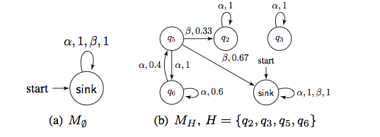
Figure 2: Two known product MDPs constructed from the example MDP (the same as the product MDP) with the sets of known states $\emptyset$ and $\{q_{2},q_{3},q_{5},q_{6}\}$ respectively.

The following lemma shows that the optimal $T$-step policy in $\mathcal{M}_{\hat{H}}$ either will be near optimal in the product MDP $\mathcal{M}$, or will allow a rapid exploration of an unknown state in $M$.

Lemma 3.

Given a product MDP $\mathcal{M}$ and a set of known states $\hat{H}\subset V$, for any $v\in\hat{H}$, for $0<\alpha<1$, let $f$ be the optimal $T$-step policy in $\mathcal{M}_{\hat{H}}$. Then, one of the following two statements holds: 1) $U_{{\cal M}}^{f}(v,T)\geq U_{\cal M}^{\ast}(v,T)-\alpha$; 2) An unknown state which is not in the accepting end state set $\mathcal{C}$ will be visited in the course of running $f$ for $T$ steps with a probability at least $\alpha$.

Proof.

Suppose that $U_{\cal M}^{f}(v,T)<U_{\cal M}^{\ast}(v,T)-\alpha$ (otherwise, $f$ witnesses the claim). First, we show for any policy $g:V\rightarrow\Sigma$, for any $v\in\hat{H}$, it holds that

$$U_{\mathcal{M}_{\hat{H}}}^{g}(v,T)\geq U_{\mathcal{M}}^{g}(v,T)$$ (1)

To prove this, for notation simplicity, let $\mathrm{Pr}=\mathrm{Pr}_{\mathcal{M}^{g}}$ be the probability measure over the paths in $\mathcal{M}^{g}$ and $\mathrm{Pr}^{\prime}=\mathrm{Pr}_{\mathcal{M}_{\hat{H}}^{g}}$ be the probability measure over the paths in $\mathcal{M}_{\hat{H}}^{g}$.

Let $X\subseteq V^{\ast}$ be a set of paths in $\mathcal{M}^{g}$ such that each $x\in X$, with $\left|x\right|\leq T$, starts in $v$, ends in $\mathcal{C}$ and has every state in $\hat{H}$; $Y\subseteq V^{\ast}$ be the set of paths in $\mathcal{M}^{g}$ such that each $y\in Y$, with $\left|y\right|\leq T$, starts in $v$, ends in $\mathcal{C}$ and has at least one state not in $\hat{H}$; and $Y^{\prime}$ be the set of paths $y$ in $\mathcal{M}^{g}_{\hat{H}}$ which starts in $v$, ends with $\mathsf{sink}$ and has length $\left|y\right|\leq T$. We can write

$$U_{\cal M}^{g}(v,T)=\sum_{x\in X}\mathrm{Pr}(x)+\sum_{y\in Y}\mathrm{Pr}(y),\text{ and }$$

$$U_{{\cal M}_{\hat{H}}}^{g}(v,T)=\sum_{x\in X}\mathrm{Pr}^{\prime}(x)+\sum_{y\in Y^{\prime}}\mathrm{Pr}^{\prime}(y).$$

Since the transition probabilities in $\mathcal{M}$ and $\mathcal{M}_{\hat{H}}$ are same for the set of known states, and $X$ is the set of paths which only visit known states, we infer that $\sum_{x\in X}\mathrm{Pr}(x)=\sum_{x\in X}\mathrm{Pr}^{\prime}(x)$. Moreover, since $y\in Y$ contains an unknown state, it leads to $\mathsf{sink}$ in $\mathcal{M}_{\hat{H}}$, and thus is in $Y^{\prime}$. We infer that $Y\subseteq Y^{\prime}$, $\sum_{y\in Y}\mathrm{Pr}(y)\leq\sum_{y\in Y^{\prime}}\mathrm{Pr}^{\prime}(y)$ and thus $U_{{\cal M}_{\hat{H}}}^{g}(v,T)\geq U_{\cal M}^{g}(v,T)$.

Next, let $f$ be the optimal $T$-step policy in $\mathcal{M}_{\hat{H}}$ and $\ell$ be the optimal $T$-step policy in $\mathcal{M}$. From Eq. (1), we obtain an inequality: $U_{\mathcal{M}_{\hat{H}}}^{\ell}(v,T)\geq U_{\mathcal{M}}^{\ell}(v,T)$.

By the $T$-step optimality of $f$ in $\mathcal{M}_{\hat{H}}$ and $\ell$ in $\mathcal{M}$, it also holds that $U_{\mathcal{M}_{\hat{H}}}^{f}(v,T)\geq U_{\mathcal{M}_{\hat{H}}}^{\ell}(v,T)$ and $U_{\mathcal{M}}^{\ast}(v,T)=U_{\mathcal{M}}^{\ell}(v,T)\geq U_{\mathcal{M}}^{f}(v,T)$. Hence,

$$U_{\mathcal{M}_{\hat{H}}}^{f}(v,T)\geq U_{\mathcal{M}_{\hat{H}}}^{\ell}(v,T)\geq U_{\mathcal{M}}^{\ast}(v,T)\geq U_{\mathcal{M}}^{f}(v,T)\\ \implies U_{\mathcal{M}_{\hat{H}}}^{f}(v,T)-U_{\mathcal{M}}^{f}(v,T)\geq U_{\mathcal{M}}^{\ast}(v,T)-U_{\mathcal{M}}^{f}(v,T).$$

Given the fact that $U_{\mathcal{M}}^{\ast}(v,T)-U_{\mathcal{M}}^{f}(v,T)>\alpha$, we infer that

$$U_{{\cal M}_{\hat{H}}}^{f}(v,T)-U_{\cal M}^{f}(v,T)=\sum_{z\in Z}\mathrm{Pr}(z)>\alpha,$$

where $Z$ is the set of paths such that each $z\in Z$ with $\left|z\right|\leq T$, $z$ starts from $v$, and ends in some unknown state which is not an accepting end state in $\mathcal{M}$. Therefore, we reach at the conclusion that if $U_{\mathcal{M}}^{f}(v,T)<U^{\ast}_{\mathcal{M}}(v,T)-\alpha$, then the probability of visiting an unknown state which is not in $\mathcal{C}$ must be at least $\alpha$. ∎

Note that, for any unknown state which is in $\mathcal{C}$, one can apply the policy in its corresponding accepting end component to visit such a state infinitely often, and after a sufficient number of visits, it will become known.

Though we use the product MDP $\mathcal{M}$ in Lemma 3, Lemma 3 can also be applied to the learned product MDP $\overline{\mathcal{M}}$.

IV PAC-MDP algorithm in control with temporal logic constraints.

Theorem 1.

Let $M=\langle Q,\Sigma,P,\mathcal{AP},L\rangle$ be an MDP with $P$ unknown, for which we aim to maximize the probability of satisfying a LTL formula $\varphi$. Let $0<\delta<1$, and $\epsilon>0$ be input parameters. Let $\mathcal{M}=M\ltimes\mathcal{A}_{\varphi}$ be the product MDP and $T$ be the $\epsilon$-state value mixing time of the optimal policy in $\mathcal{M}$. Let $F_{\cal M}(\epsilon,T)$ be the set of policies in $\cal M$ whose $\epsilon$-state value mixing time is $T$. With probability no less than $1-\delta$, Algorithm 1 will return a policy $f\in F_{\cal M}(\epsilon,T)$ such that $\left|U^{f}_{\mathcal{M}}(v,T)-U^{\ast}_{\mathcal{M}}(v)\right|\leq 3\epsilon$ within a number of steps polynomial in $\left|Q\right|$, $\left|\Sigma\right|$, $\left|S\right|$, $T$, $\frac{1}{\epsilon}$ and $\frac{1}{\delta}$.

Proof.

Firstly, applying the Chernoff bound [17], the upper bound on the number of visits to a state for it to be known is polynomial in $\left|\Sigma\right|,T,\frac{1}{\epsilon}$ and $\frac{1}{\delta}$. Before all states are known, the current policy $f$ exercised by the system is $T$-step optimal in $\overline{\mathcal{M}}_{\hat{H}}$ induced from the set of known states $\hat{H}$. Then, by Lemma 3, either for each state, policy $f$ attains a state value $\alpha$-close to the optimal $T$-step state value in $\overline{\mathcal{M}}$, or an unknown state will be visited with probability at least $\alpha$. However, because $\overline{\mathcal{M}}_{\hat{H}}$ is $\frac{\epsilon}{NT}$-approximation of $\mathcal{M}_{\hat{H}}$, Lemma 1 and Lemma 2 guarantee that policy $f$ either attains a state value $(2\epsilon+\alpha)$-close to the optimal $T$-step state value in $\mathcal{M}$ for any state, or explores efficiently. If it is always not the first case, then after a finite number of steps, which is polynomial in $\left|Q\right|,\left|\Sigma\right|,T,\frac{1}{\epsilon},\frac{1}{\delta}$, all states will be known, and the learned MDP $\overline{M}$ (resp. $\overline{\mathcal{M}}$) $\frac{\epsilon}{NT}$-approximates the true MDP $M$ (resp. $\mathcal{M}$). Since $T$ is the $\epsilon$-state value mixing time of the optimal policy in $\mathcal{M}$, the $T$-step optimal policy $g:V\rightarrow\Sigma$ in $\mathcal{M}$ satisfies $\left|U_{\mathcal{M}}^{g}(v,T)-U_{\mathcal{M}}^{\ast}(v)\right|\leq\epsilon$. From Lemma 2, it holds that $\left|U_{\mathcal{M}}^{f}(v,T)-U_{\mathcal{M}}^{g}(v,T)\right|\leq 2\epsilon$ and thus we infer that $\left|U_{\mathcal{M}}^{f}(v,T)-U_{\mathcal{M}}^{\ast}(v)\right|\leq 3\epsilon$. ∎

Note that, the sample complexity of the algorithm is polynomial in $\left|Q\right|,\left|\Sigma\right|,T,\frac{1}{\epsilon},\frac{1}{\delta}$, unrelated to the size of $\mathcal{A}_{\varphi}$. However, in the value iteration step, the space and time complexity of policy synthesis is polynomial in $\left|Q\right|,\left|S\right|,\left|\Sigma\right|,T,\frac{1}{\epsilon},\frac{1}{\delta}$.

In problem 1, we aim to obtain a policy $f$ which is $\varepsilon$-optimal in $\mathcal{M}$. This can be achieved by setting $\epsilon=\frac{\varepsilon}{3}$ (see Theorem 1).

In Algorithm 1, policy is updated at most $\left|Q\right|$ times as there is no need to update it if a new observation does not cause an unknown state to become known. Given the fact that for LTL specifications, the time and space complexity of synthesis is polynomial in the size of the product MDP, Algorithm 1 is a provably efficient algorithm for learning and policy update.

Similar to [1, 2], the input $T$ can be eliminated by either estimating an upper bound for $T$ or starting with $T=1$ and iteratively increase $T$ by $1$. The reader can refer to [1, 2] for more detailed discussion on the elimination technique.

Input: The state and action sets $Q$ ,$\Sigma$, the set of atomic propositions $\mathcal{AP}$ and the labeling function $L:Q\rightarrow 2^{\mathcal{AP}}$, the specification DRA $\mathcal{A}_{\varphi}$, parameters $\epsilon$ and $\delta$, the (upper bound of) $\epsilon$-state mixing time $T$ for the optimal policy in $M\ltimes\mathcal{A}_{\varphi}$.

Output: A policy $f:Q\times S\rightarrow\Sigma$.

begin

       $H:=\emptyset$, $q:=q_{0}$, $s:=I_{s}$, recompute=True;

      $\overline{M}=\langle Q,\Sigma,\overline{P},\mathcal{AP},L\rangle$, /* $\overline{P}(q,a,q^{\prime})=0$ for any $(q,a,q^{\prime})\in Q\times\Sigma\times Q$. */

      

      while True do

             $s:=T_{s}(s,L(q))$,

            if recompute=True then

                   $\hat{H}=H\times S$, $\overline{\mathcal{M}}=\overline{M}\ltimes\mathcal{A}_{\varphi}$, $\overline{\mathcal{M}}_{\hat{H}}:=\textnormal{{KnownMDP}}(\overline{\mathcal{M}},\hat{H})$, $f:=\textnormal{{ValueIteration}}(\overline{\mathcal{M}}_{\hat{H}},T)$

            

            $q^{\prime},a=\textnormal{{Exploit}}((q,s),f)$, $H_{p}=H$, $\overline{M},H:=\textnormal{{Update}}(\overline{M},H,q,a,q^{\prime},\epsilon,\delta,\left|Q\right|,T)$

            if $H_{p}\neq H$ then recompute=True;

            else recompute=False;

             if $\overline{P}(q^{\prime},a,q^{\prime})=1$ or $(q,s)\in\overline{\mathcal{C}}$ then With probability $0\leq p\leq 1$, restart with a random state in $Q$ and set $s=I_{s}$, else $q:=q^{\prime}$;

            else  $q:=q^{\prime}$;

             ;

              /* $\overline{\mathcal{C}}$ is the accepting end states in $\overline{M}$. */

            

            if $H=Q$ then

                   return $f:=\textnormal{{ValueIteration}}(\overline{\mathcal{M}},T).$

            

      

Algorithm 1 LearnAndSynthesis

During learning, it is possible that for state $q\in Q$ and for action $a\in\Sigma$, we estimate that $\overline{P}(q,a,q)=1$. Then either in the true MDP, $P(q,a,q)=1$, or, $P(q,a,q)<1$ yet we have not observed a transition $(q,a,q^{\prime})$ for any $q^{\prime}\neq q$. In this case, with some probability $p$, we restart with a random initial state of MDP. With probability $1-p$, we keep exploring state $q$. The probability $p$ is a tuning parameter in Algorithm 1.

V Examples

We apply Algorithm 1 to the running example MDP (Fig. 1) and a robotic motion planning problem in an unknown terrain. The implementations are in Python on a desktop with Intel(R) Core(TM) processor and $16$ GB of memory.

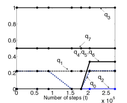
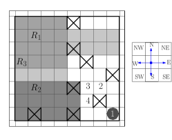
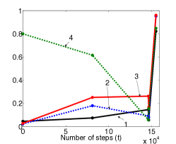
Figure 3: (a) The state value $U_{\mathcal{M}}^{f^{t}}(q_{i})$, $i=0,\ldots,7$ v.s. step $t$, with $\varepsilon=0.01$, $\delta=0.05$ and $T=15$. The markers represents the steps when the policy is recomputed. Note that, for states $q_{0}$ and $q_{1}$, the state values at $t_{f}$ are $0.22445$ and $0.22$ respectively, which are indiscernible from the figure. (b) Left: A $10\times 10$ gridworld, where the disk represents the robot, the cells $R_{1}$, $R_{2}$, and $R_{3}$ are the interested regions, the crossed cells are the obstacles, labeled with $R_{4}$, the cells on the edges are walls, and we assume that if the robot hits the wall, it will be bounced back to the previous cell. Different grey scales represents different terrains: From the darkest to the lightest, these are “grass,” “ pavement,” “sand” and “gravel.” Right: The transitions of the robot, in which the center cell is the current location of the robot. (c) The state value $U_{\mathcal{M}}^{f^{t}}((q_{0},s_{0}))$ v.s. step $t$, where $q_{0}\in\{1,2,3,4\}$ is the initial cell and $s_{0}=T_{s}(I_{s},L(q_{0}))$, under $\epsilon=0.01$, $\delta=0.05$ and $T=50$. The markers represents the steps when the policy is recomputed.

V-A The running example

We consider different assignments for $\varepsilon$ and $95\%$ of confidence level, i.e., $\delta=0.05$, and $T=15$ as the (estimated upper bound of) $\frac{\varepsilon}{3}$-state value mixing time of the optimal policy, for all assignments of $\varepsilon$. A step means that the system takes an action and arrives at a new state.

For $\varepsilon=0.01$, after $t_{f}=274968$ steps, all states become known and the policy update terminates after $8$ updates and $35.12$ seconds. Let the policy at step $t$ be denoted as $f^{t}$. We evaluate the policy $f^{t}$ in the true product-MDP and plot the state value (the probability of satisfying the specification from that state under policy $f^{t}$) $U_{\mathcal{M}}^{f^{t}}(q_{i}):i=0,\ldots,7$, for the finite horizon $[0,t_{f}]$ in Fig. 3. Note that, even though the policy computed at step $t=204468$ has already converged to the optimal policy, it is only after $t=t_{f}=274968$ that in the system’s hypothesis, the $T$-step state value computed using the known MDP with its $T$-step optimal policy converges $\varepsilon$-close to the optimal state value in the true product MDP.

For $\varepsilon=0.02$, in $136403$ steps with $17.73$ seconds, all states become known and the policy is the optimal one. For $\varepsilon=0.05$, in $55321$ steps with $7.18$ seconds all states are known. However, the policy $f$ outputs $\alpha$ for all states except $q_{5}$, at which it outputs $\beta$. Comparing to the optimal policy which outputs $\beta$ for both $q_{0}$ and $q_{5}$, $f$ is sub-optimal in the true MDP $\mathcal{M}$: With $f$, $U_{\mathcal{M}}^{f}(q_{0})=0.22$, comparing to $0.22445$ with the optimal policy. For the remaining states, we obtain the same state values with policy $f$ as the optimal one.

Finally, in three experiments, it is observed that the actual maximal error ($0.00445$ with $\varepsilon=0.05$) never exceeds $0.01$, because we use the loose upper bound on the error between the $T$-step state value with any policy in $\mathcal{M}$ and its approximation $\overline{\mathcal{M}}$ in Lemma 1, to guarantee the correctness of the solution.

V-B A motion planning example

We apply the algorithm to a robot motion planning problem (see Fig. 3). The environment consists of four different unknown terrains: Pavement, grass, gravel and sand. In each terrain and for robot’s different action (heading north (‘N’), south (‘S’), west (‘W’) and east (‘E’)), the probability of arriving at the correct cell is in certain ranges: $[0.9,0.95]$ for pavement, $[0.85,0.9]$ for grass, $[0.8,0.85]$ for gravel and $[0.75,0.80]$ for sand. With a relatively small probability, the robot will arrive at the cell adjacent to the intended one. For example, with action ‘N’, the intended cell is the one to the north (‘N’), whose the adjacent ones are the northeast (‘NE’)and northwest cells (‘NW’) (see Fig. 3). The objective of the robot is to maximize the probability of satisfying a temporal logic specification $\varphi=\square\lozenge(R_{1}\land\lozenge(R_{2}\land\lozenge R_{3}))\land\square\neg R_{4}$ where $R_{1},R_{2},R_{3}$ are critical surveillance cells and $R_{4}$ includes a set of unsafe cells to be avoided. For illustrating the effectiveness of the algorithm, we mark a subset of cells labeled by $1,2,3,4$ and evaluate the performance of iteratively updated policies given that a cell in the set is the initial location of the robot.

Given $\varepsilon=0.01$, $\delta=0.05$, and $T=50$, all states become known in $t_{f}=155089$ steps and $1593.45$ seconds, and the policy updated four times (one for each terrain type). It is worth mentioning that most of the computation time is spent on computing the set of bottom strongly connected components using the algorithm in [12] in the structure of the learned MDP, which is then used to determine the set of accepting end components in $\overline{\mathcal{M}}$. In Fig. 3, we plot the state value $U_{\mathcal{M}}^{f^{t}}((q_{0},s_{0}))$ where $q_{0}\in\{1,2,3,4\}$ and $s_{0}=T_{s}(I_{s},q_{0})$ for a finite time horizon. The policy output by Algorithm 1 is the optimal policy in the true MDP. The video demonstration for this example is available at http://goo.gl/rVMkrT.

VI Conclusion and future work

We presented a PAC-MDP method for synthesis with temporal logic constraints in unknown MDPs and developed an algorithm that integrates learning and control for obtaining approximately optimal policies for temporal logic constraints with polynomial time, space and sample complexity. Our current work focuses on other examples (e.g. multi-vehicle motion planning), comparison to alternative, possibly ad hoc methods, and implementing a version of Algorithm 1 that circumvents the need for the input $T$ following [2].

There are a number of interesting future extensions. First, although here we only considered one-player stochastic games, it is also possible to extend to two-player stochastic games, similar to the R-max algorithm [2]. The challenge is that in two-player stochastic games, only considering deterministic, memoryless policies in the product-MDP may not be sufficient. For the synthesis algorithm, different strategy classes (memoryless, finite-memory, combined with deterministic and randomized) require different synthesis methods. We may need to integrate this PAC-MDP approach with other synthesis methods for randomized, finite-memory strategies. Second, besides the objective of maximizing the probability of satisfying a temporal logic constraint, other objectives can be considered, for example, minimizing the weighted average costs [18]. Third, the method is model-based in the sense that a hypothesis for the underlying MDP is maintained. The advantage in such a model-based approach is that when the control objective is changed, the knowledge gained in the past can be re-used in the policy synthesis for the new objective. However, model-free PAC-MDP approach [19], in which information on the policy is retained directly instead of the transition probabilities, can be of interests as its space-complexity is asymptotically less than the space requirement for model-based approaches.

Proof of Lemma 1.

By Definition 6, $M$ and $\overline{M}$ share the same structure. Thus, for any DRA $\mathcal{A}_{\varphi}$, the product MDPs $\mathcal{M}=M\ltimes\mathcal{A}_{\varphi}$ and $\overline{\mathcal{M}}=\overline{M}\ltimes\mathcal{A}_{\varphi}$ share the same structure and the same set of accepting end states $\mathcal{C}\subseteq V$.

For any policy $f$, let $M_{i}$ be the Markov chains obtained from the induced Markov chains $\mathcal{M}^{f}$ and $\overline{\mathcal{M}}^{f}$ in the following way: Start at $v$ and for the first $i$ transitions, the transition probabilities are the same as in $\overline{\mathcal{M}}^{f}$, and for the rest of steps, the transition probabilities are the same as in $\mathcal{M}^{f}$. Clearly, $\mathcal{M}^{f}=M_{0}$ and $\overline{\mathcal{M}}^{f}=M_{T}$. For notational simplicity, we denote $h_{M_{i}}(\cdot)=h_{i}(\cdot)$, $\mathrm{Pr}_{M_{i}}(\cdot)=\mathrm{Pr}_{i}(\cdot)$. Then, we have that

$$\left|U_{\cal M}^{f}(v,T)-U_{\overline{\cal M}}^{f}(v,T)\right|=\left|h_{0}^{\leq T}(v,\mathcal{C})-h_{T}^{\leq T}(v,\mathcal{C})\right|$$

$$= \left|h_{0}^{\leq T}(v,\mathcal{C})-h_{1}^{\leq T}(v,\mathcal{C})+h_{1}^{\leq T}(v,\mathcal{C})-h_{2}^{\leq T}(v,\mathcal{C})+\ldots+\right.$$

$$\left.h_{T-1}^{\leq T}(v,\mathcal{C})-h_{T}^{\leq T}(v,\mathcal{C})\right|=\sum_{i=0}^{T-1}\left|h_{i}^{\leq T}(v,\mathcal{C})-h_{i+1}^{\leq T}(v,\mathcal{C})\right|$$

$$\leq T\cdot\max_{i\in\{0,\ldots T-1\}}\left|h_{i}^{\leq T}(v,\mathcal{C})-h_{i+1}^{\leq T}(v,\mathcal{C})\right|.$$ (2)

For any $i=0,\ldots,T-1$, we have that

$$\small\mathsf{Diff1}=\left|h_{i}^{\leq T}(v,\mathcal{C})-h_{i+1}^{\leq T}(v,\mathcal{C})\right|=\left|h_{i}^{\leq i}(v,\mathcal{C})\right.\\ \left.+\sum_{k=i+1}^{T}h_{i}^{k}(v,\mathcal{C})-h_{i+1}^{\leq i}(v,\mathcal{C})-\sum_{k=i+1}^{T}h_{i+1}^{k}(v,\mathcal{C})\right|.$$

Since for the first $i$ steps, the transition probabilities in $M_{i}$ and $M_{i+1}$ are the same, then the probabilities of hitting the set $\mathcal{C}$ in $M_{i}$ and $M_{i+1}$ equal to the probability of hitting $\mathcal{C}$ in $\mathcal{M}^{f}=M_{0}$, i.e., $h_{i}^{\leq i}(v,\mathcal{C})=h_{i+1}^{\leq i}(v,\mathcal{C})=h_{0}^{\leq i}(v,\mathcal{C})$. Remind that $\mathrm{Pr}_{i}(x)$, for some $x\in V^{\ast}$, is the probability of path $x$ occurring in $M_{i}$, as a consequence,

$$\small\begin{split}&\mathsf{Diff1}=\left|\sum_{k=i+1}^{T}h_{i}^{k}(v,\mathcal{C})-\sum_{k=i+1}^{T}h_{i+1}^{k}(v,\mathcal{C})\right|\\ =&\left|\sum_{v^{\prime}\notin\mathcal{C}}\mathrm{Pr}_{i}(xv^{\prime})\sum_{v^{\prime\prime}\notin\mathcal{C}}\big{(}\mathrm{Pr}_{i}(v^{\prime}v^{\prime\prime})\cdot h_{i}^{\leq T-i-1}(v^{\prime\prime},\mathcal{C})\big{)}-\right.\\ &\left.\sum_{v^{\prime}\notin\mathcal{C}}\mathrm{Pr}_{i+1}(xv^{\prime})\sum_{v^{\prime\prime}\ \notin\mathcal{C}}\big{(}\mathrm{Pr}_{i+1}(v^{\prime}v^{\prime\prime})\cdot h_{i+1}^{\leq T-i-1}(v^{\prime\prime},\mathcal{C})\big{)}\right|,\end{split}$$

where $x\in V^{\ast}$ is a path of length $i-1$ that starts in $v$ and does not contain any state in $\mathcal{C}$. Note that for the first $i$ (resp. the last $T-i-1$) transitions, the transition probabilities in $M_{i}$ and $M_{i+1}$ are the same as these in $\mathcal{M}^{f}=M_{0}$ (resp. $\overline{\mathcal{M}}^{f}=M_{T}$), thus we have $\mathrm{Pr}_{i}(xv^{\prime})=\mathrm{Pr}_{i+1}(xv^{\prime})=\mathrm{Pr}_{0}(xv^{\prime})$ and $h_{i}^{\leq T-i-1}(v^{\prime\prime},\mathcal{C})=h_{i+1}^{\leq T-i-1}(v^{\prime\prime},\mathcal{C})=h_{T}^{\leq T-i-1}(v^{\prime\prime},\mathcal{C})$ .

Let $v^{\prime}=(q^{\prime},s^{\prime})$, $v^{\prime\prime}=(q^{\prime\prime},s^{\prime\prime})$ and $a=f(v^{\prime})$. It is also noted that $\mathrm{Pr}_{i}(v^{\prime}v^{\prime\prime})=\mathrm{Pr}_{i}((q^{\prime},s^{\prime})(q^{\prime\prime},s^{\prime\prime}))=P(q^{\prime},a,q^{\prime\prime})$ with $s^{\prime\prime}=T_{s}(s^{\prime},L(q^{\prime\prime}))$ and $\mathrm{Pr}_{i+1}(v^{\prime}v^{\prime\prime})=\mathrm{Pr}_{i+1}((q^{\prime},s^{\prime})(q^{\prime\prime},s^{\prime\prime}))=\overline{P}(q^{\prime},a,q^{\prime\prime})$. Thus, as $\overline{M}$ approximate $M$, we have

$$\small\begin{split}&\mathsf{Diff1}=\sum_{v^{\prime}\notin\mathcal{C}}\mathrm{Pr}_{0}(xv^{\prime})\sum_{v^{\prime\prime}\notin\mathcal{C}}\big{(}\left|P(q^{\prime},a,q^{\prime\prime})-\overline{P}(q^{\prime},a,q^{\prime\prime})\right|\\ &\cdot h_{T}^{\leq T-i-1}(v^{\prime\prime},\mathcal{C})\big{)}\\ \leq&\sum_{v^{\prime}\notin\mathcal{C}}\mathrm{Pr}_{0}(xv^{\prime})\cdot\frac{\epsilon}{NT}\cdot\sum_{v^{\prime\prime}\notin\mathcal{C}}h_{T}^{\leq T-i-1}(v^{\prime\prime},\mathcal{C})=\mathsf{Diff2},\end{split}$$

The first term $\sum_{v^{\prime}\notin\mathcal{C}}\mathrm{Pr}_{0}(xv^{\prime})\leq 1$ and the last term is the sum of the probabilities of visiting $\mathcal{C}$ from different states in $V\setminus\mathcal{C}$ within $T-i-1$ steps, each of which is bounded by $1$. Moreover, since $v^{\prime\prime}=(q^{\prime\prime},s^{\prime\prime})$ where $s^{\prime\prime}$ is determined by the previous state $s^{\prime}$ in $\mathcal{A}_{\varphi}$ and the current state $q^{\prime\prime}$, i.e., $s^{\prime\prime}=T_{s}(s^{\prime},L(q^{\prime\prime}))$, the sum is bounded by the number $N$ of states (choices for $q^{\prime\prime}$) in the underlying MDP $M$. Thus, $\mathsf{Diff1}\leq\mathsf{Diff2}\leq\frac{\epsilon}{NT}\cdot N=\frac{\epsilon}{T}$. Finally, from (2), we have $\left|U_{\cal M}^{f}(v,T)-U_{\overline{\cal M}}^{f}(v,T)\right|\leq\frac{\epsilon}{T}\cdot T=\epsilon$. ∎

References

- [1] M. Kearns and S. Singh, “Near-optimal reinforcement learning in polynomial time,” Machine Learning, vol. 49, pp. 209–232, Nov. 2002.
- [2] R. Brafman and M. Tennenholtz, “R-MAX-a general polynomial time algorithm for near-optimal reinforcement learning,” The Journal of Machine Learning, vol. 3, pp. 213–231, 2003.
- [3] A. Legay, B. Delahaye, and S. Bensalem, “Statistical model checking: An overview,” in Runtime Verification, pp. 122–135, Springer, 2010.
- [4] D. Henriques, J. G. Martins, P. Zuliani, A. Platzer, and E. M. Clarke, “Statistical model checking for Markov decision processes,” International Conference on Quantitative Evaluation of Systems, pp. 84–93, Sept. 2012.
- [5] Y. Chen, J. Tumova, and C. Belta, “LTL robot motion control based on automata learning of environmental dynamics,” in IEEE International Conference on Robotics and Automation, pp. 5177–5182, May 2012.
- [6] J. Fu, H. G. Tanner, and J. Heinz, “Adaptive planning in unknown environments using grammatical inference,” in IEEE Conference on Decision and Control, 2013.
- [7] H. Mao, Y. Chen, M. Jaeger, T. D. Nielsen, K. G. Larsen, and B. Nielsen, “Learning markov decision processes for model checking,” in Proceedings of Quantities in Formal Methods (U. Fahrenberg, A. Legay, and C. R. Thrane, eds.), Electronic Proceedings in Theoretical Computer Science, pp. 49–63, 2012.
- [8] J. Rutten, M. Kwiatkowska, G. Norman, and D. Parker, Mathematical Techniques for Analyzing Concurrent and Probabilistic Systems, P. Panangaden and F. van Breugel (eds.), vol. 23 of CRM Monograph Series. American Mathematical Society, 2004.
- [9] C. Baier, M. Größer, M. Leucker, B. Bollig, and F. Ciesinski, “Controller Synthesis for Probabilistic Systems (Extended Abstract),” in Exploring New Frontiers of Theoretical Informatics (J.-J. Levy, E. Mayr, and J. Mitchell, eds.), vol. 155 of International Federation for Information Processing, pp. 493–506, Springer US, 2004.
- [10] A. Bianco and L. De Alfaro, “Model checking of probabilistic and nondeterministic systems,” in Foundations of Software Technology and Theoretical Computer Science, pp. 499–513, Springer, 1995.
- [11] L. De Alfaro, Formal Verification of Probabilistic Systems. PhD thesis, Stanford University, 1997.
- [12] K. Chatterjee, M. Henzinger, M. Joglekar, and N. Shah, “Symbolic algorithms for qualitative analysis of Markov decision processes with Büchi objectives,” Formal Methods in System Design, vol. 42, no. 3, pp. 301–327, 2012.
- [13] M. O. Duff, Optimal Learning: Computational Procedures for Bayes-adaptive Markov Decision Processes. PhD thesis, University of Massachusetts Amherst, 2002.
- [14] T. Wang, D. Lizotte, M. Bowling, and D. Schuurmans, “Bayesian sparse sampling for on-line reward optimization,” in Proceedings of the 22nd International Conference on Machine Learning, pp. 956–963, ACM, 2005.
- [15] P. S. Castro and D. Precup, “Using linear programming for bayesian exploration in markov decision processes,” in International Joint Conferences on Artificial Intelligence (M. M. Veloso, ed.), pp. 2437–2442, 2007.
- [16] N. Balakrishnan and V. B. Nevzorov, A Primer on Statistical Distributions. Wiley, 2004.
- [17] B. L. Mark and W. Turin, Probability, Random Processes, and Statistical Analysis. Cambridge University Press Textbooks, 2011.
- [18] E. M. Wolff, U. Topcu, and R. M. Murray, “Optimal control with weighted average costs and temporal logic specifications.,” in Robotics: Science and Systems, 2012.
- [19] A. L. Strehl, L. Li, E. Wiewiora, J. Langford, and M. L. Littman, “PAC model-free reinforcement learning,” in Proceedings of the 23rd International Conference on Machine Learning, pp. 881–888, ACM, 2006.