On the use of charged-track information
to subtract neutral pileup

Abstract

The use of charged pileup tracks in a jet to predict the neutral pileup component in that same jet could potentially lead to improved pileup removal techniques, provided there is a strong local correlation between charged and neutral pileup. In Monte Carlo simulation we find that the correlation is however moderate, a feature that we attribute to characteristics of the underlying non-perturbative dynamics. Consequently, ‘neutral-proportional-to-charge’ (NpC) pileup mitigation approaches do not outperform existing, area-based, pileup removal methods. This finding contrasts with the arguments made in favour of a new method, “jet cleansing”, in part based on the NpC approach. We identify the critical differences between the performances of linear cleansing and trimmed NpC as being due to the former’s rejection of subjets that have no charged tracks from the leading vertex, a procedure that we name “zeroing”. Zeroing, an extreme version of the “charged-track trimming” proposed by ATLAS, can be combined with a range of pileup-mitigation methods, and appears to have both benefits and drawbacks. We show how the latter can be straightforwardly alleviated. We also discuss the limited potential for improvement that can be obtained by linear combinations of the NpC and area-subtraction methods.

1 Introduction

Pileup, the superposition of many soft proton–proton collisions over interesting hard-scattering events, is a significant issue at CERN’s Large Hadron Collider (LHC) and also at possible future hadron colliders. It affects many observables, including lepton and photon isolation, missing-energy determination and especially jet observables. One main technique currently in use to remove pileup from jet observables [1, 2] is known as the area–median approach [3, 4]. It makes an event-wide estimate of the pileup level, $\rho$, and then subtracts an appropriate 4-momentum from each jet based on its area, i.e. its extent in rapidity and azimuth.

Detector-level information can also help mitigate the effect of pileup: for example, with methods such as particle flow [5] reconstruction, it is to some extent possible to eliminate the charged component of pileup, through the subtraction of contributions from individual charged pileup hadrons. However, even with such charged hadron subtraction (CHS), there is always a substantial remaining (largely) neutral pileup contribution, which remains to be removed. Currently, when CHS is used, area–median subtraction is then applied to remove the remaining neutral pileup.

Another approach is to use the information about charged pileup hadrons in a specific jet to estimate and subtract the remaining neutral component, without any reference to a jet area or a global event energy density $\rho$. Its key assumption is that the neutral energy flow is proportional to the charged energy flow and so we dub it neutral-proportional-to-charged (NpC) subtraction. An advantage that one might imagine for NpC subtraction is that, by using local information about the charged pileup, it might be better able to account for variations of the pileup from point-to-point within the event than methods that rely on event-wide pileup estimates. We understand that there has been awareness of this kind of approach in the ATLAS and CMS collaborations for some time now, and we ourselves also investigated it some years ago [8]. Our main finding was that at particle level it performed marginally worse than area subtraction combined with CHS. From discussions with colleagues in the experimental collaborations, we had the expectation that there might be further degradation at detector level. Accordingly we left our results unpublished.

Recently Ref. [9] (KLSW) made a proposal for an approach to pileup removal named Jet Cleansing. One of the key ideas that it uses is precisely the NpC method, applied to subjets, much in the way that area–median subtraction has in the past [12, 13] been used with filtering [14] and trimming [15]. KLSW found that cleansing brought large improvements over area–median subtraction.

Given our earlier findings, KLSW’s result surprised us. The purpose of this article is therefore to revisit our study of the NpC method and also carry out independent tests of cleansing, both to examine whether we reproduce the large improvements that they observed and to identify possible sources of differences. As part of our study, we will investigate what properties of events can provide insight into the performance of the NpC method. We will also be led to discuss the possible value of charged tracks from the leading vertex in deciding whether to keep or reject individual subjets (as in charged-track based trimming of Ref. [11]). Finally we shall also examine how one might optimally combine NpC and area–median subtraction.

2 The Neutral-proportional-to-Charged method

NpC subtraction relies on the experiments’ ability to identify whether a given charged track is from a pileup vertex, in order to measure the charged pileup entering a particular jet. To a good extent this charged component can be removed, for example as in CMS’s Charged-Hadron Subtraction (CHS) procedure in the context of particle flow [5]. The NpC method then further estimates and subtracts the neutral pileup component by assuming it to be proportional to the charged pileup component. At least two variants can be conceived of.

If the charged pileup particles are kept as part of the jet during clustering, then the corrected jet momentum is [8]

$$p_{\mu}^{\text{jet,sub}}=p_{\mu}^{\text{jet}}-\frac{1}{\gamma_{0}}p_{\mu}^{\text{jet,chg-PU}}\,,$$ (1)

where $p_{\mu}^{\text{jet,chg-PU}}$ is the four-momentum of the charged-pileup particles in the jet and $\gamma_{0}$ is the average fraction of pileup transverse momentum that is carried by charged particles. Specifically, one can define

$$\gamma_{0}\equiv\left\langle\frac{\sum_{i\in\text{charged particles}}\,p_{ti}}{\sum_{i\in\text{all particles}}\,p_{ti}}\right\rangle_{\text{\!\!events}}\!\!\!\!\!,$$ (2)

where the sums run over particles in a given event (possibly limited to some central region with tracking), and the average is carried out across minimum-bias events.

If the charged pileup particles are not directly included in the clustering (i.e. it is the CHS event that is provided to the clustering), then one does not have any information on which charged particles should be used to estimate the neutral pileup in a given jet. This problem can be circumvented by a clustering an “emulated” CHS event, in which the charged-pileup particles are kept, but with their momenta rescaled by an infinitesimal factor $\epsilon$. In this case the correction becomes

$$p_{\mu}^{\text{jet,sub}}=p_{\mu}^{\text{jet,CHS}}-\frac{1-\gamma_{0}}{\gamma_{0}\,\epsilon}p_{\mu}^{\text{jet,rescaled-chg-PU}}\,,$$ (3)

where $p_{\mu}^{\text{jet,CHS}}$ is the momentum of the jet as obtained from the emulated CHS event, while $p_{\mu}^{\text{jet,rescaled-chg-PU}}$ is the summed momentum of the rescaled charged-pileup particles that are in the jet. When carrying out NpC-style subtraction, this is our preferred approach because it eliminates any backreaction associated with the charged pileup (this is useful also for area-based subtraction), while retaining the information about charged pileup tracks.

There are multiple issues that may be of concern for the NpC method. For example, calorimeter fluctuations can limit the experiments’ ability to accurately remove the charged pileup component as measured with tracks. For out-of-time pileup, which contributes to calorimetric energy deposits, charged-track information may not be available at all. In any case, charged-track information covers only a limited range of detector pseudorapidities. Additionally there are subtleties with hadron masses: in effect, $\gamma_{0}$ is different for transverse components and for longitudinal components. In this work we will avoid this problem by treating all particles as massless. The importance of the above limitations can only be fully evaluated in an experimental context.

We will be comparing NpC to the area–median method. The latter makes a global estimate of pileup transverse-momentum flow per unit area, $\rho$, by dividing an event into similarly sized patches and taking the median of the transverse-momentum per unit area across all the patches. It then corrects each jet using the globally estimated $\rho$ and the individual jet’s area, $A_{\mu}$,

$$p_{\mu}^{\text{jet,sub}}=p_{\mu}^{\text{jet}}-\rho A_{\mu}\,.$$ (4)

Like NpC, the area–median method has potential experimental limitations. They include include questions of non-trivial rapidity dependence and detector non-linearities (the latter are relevant also for NpC). These have, to a reasonable extent, been successfully overcome by the experiments [1, 2]. One respect in which NpC may have advantages over the area–median method is that the latter fails to correctly account for the fact that pileup fluctuates from point to point within the event, a feature that cannot be encoded within the global pileup estimate $\rho$. Furthermore NpC does not need a separate estimation of the background density $\rho$, which can have systematics related to the event structure (e.g. $t\bar{t}$ events v. dijet events); and there is no need to include large numbers of ghosts for determining jet areas, a procedure that has a non-negligible computational cost.

Let us now proceed with an investigation of NpC’s performance, focusing our attention on particle-level events for simplicity. The key question is the potential performance gain due to NpC’s use of local information. To study this quantitatively, we consider a circular patch of radius $R$ centred at $y=\phi=0$ and examine the correlation coefficient of the actual neutral energy flow in the patch with two estimates: (a) one based on the charged energy flow in the same patch and (b) the other based on a global energy flow determination from the neutral particles, $\rho_{\text{ntr}}$. Fig. 1 (left) shows these two correlation coefficients, “ntr v. chg” and “ntr v. $\rho_{\text{ntr}}A$”, as a function of $R$, for two average pileup multiplicities, $\mu=20$ and $\mu=100$. One sees that the local neutral-charged correlation is slightly lower, i.e. slightly worse, than the neutral-$\rho_{\text{ntr}}$ correlation. Both correlations decrease for small patch radii, as is to be expected, and the difference between them is larger at small patch radii. The correlation is largely independent of the number of pileup events being considered, which is consistent with our expectations, since all individual terms in the determination of the correlation coefficient should have the same scaling with $N_{\text{PU}}$.

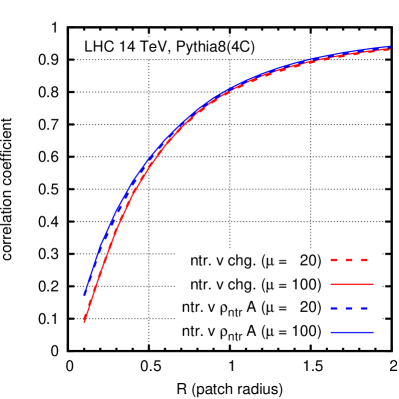
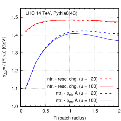
Figure 1: Left: the correlation coefficient between the neutral transverse momentum in a central patch and either the charged transverse momentum in that patch (rescaling this component would not change the value of the correlation coefficient) or the prediction using the area–median method, i.e. $\rho_{\text{ntr}}A$. Right: the standard deviation of the difference between neutral transverse momentum in a central patch and either the rescaled charged transverse momentum in that patch or the prediction using the area–median method, i.e. $\rho_{\text{ntr}}A$. The events are composed of superposed zero-bias collisions simulated with Pythia 8, tune 4C, and the number of collisions per event is Poisson distributed with average $\mu$.

Quantitative interpretations of correlation coefficients can sometimes be delicate, as we discuss in Appendix B, essentially because they combine the covariance of two observables with the two observables’ individual variances. We find that it can be more robust to investigate a quantity $\sigma_{\Delta p_{t}^{\text{ntr}}}$, the standard deviation of

$$\Delta p_{t}^{\text{ntr}}=p_{t}^{\text{ntr}}-p_{t}^{\text{ntr,estimated}}\,,$$ (5)

where the estimate of neutral energy flow, $p_{t}^{\text{ntr,estimated}}$, may be either from the rescaled charged flow or from $\rho_{\text{ntr}}A$. The right-hand plot of Fig. 1 shows $\sigma_{\Delta p_{t}^{\text{ntr}}}$ for the two methods, again as a function of $R$, for two levels of pileup. It is normalised to $R\sqrt{\mu}$, to factor out the expected dependence on both the patch radius and the level of pileup. A lower value of $\sigma_{\Delta p_{t}^{\text{ntr}}}$ implies better performance, and as with the correlation we reach the conclusion that a global estimate of $\rho_{\text{ntr}}$ appears to be slightly more effective at predicting local neutral energy flow than does the local charged energy flow. If one hoped to use NpC to improve on the performance of area–median subtraction, then figure 1 suggests that one will be disappointed.

In striving for an understanding of this finding, one should recall that the ratio of charged-to-neutral energy flow is almost entirely driven by non-perturbative effects. Inside an energetic jet, the non-perturbative effects are at scales $\sim\Lambda_{\text{QCD}}$ that are tiny compared to the jet transverse momentum $p_{t}$. There are fluctuations in the relative energy carried by charged and neutral particles, for example because a leading $u$-quark might pick up a $\bar{d}$ or a $\bar{u}$ from the vacuum. However, because $\Lambda_{\text{QCD}}\ll p_{t}$, the charged and neutral energy flow mostly tend to go in the same direction.

The case that we have just seen of an energetic jet gives an intuition that fluctuations in charged and neutral energy flow are going to be locally correlated. It is this intuition that motivates the study of NpC. We should however examine if this intuition is actually valid for pileup. We will examine one step of hadronisation, namely the production of short-lived hadronic resonances, for example a $\rho^{+}$. The opening angle between the $\pi^{+}\pi^{0}$ decay products of the $\rho^{+}$ is of order $2m_{\rho}/p_{t,\rho}$. Given that pileup hadrons are produced mostly at low $p_{t}$, say $0.5-2\,\text{GeV}$, and that $m_{\rho}\simeq 0.77\,\text{GeV}$, the angle between the charged and neutral pions ends up being of order $1$ or even larger. As a result, the correlation in direction between charged and neutral energy flow is lost, at least in part. Thus, at low $p_{t}$, non-perturbative effects specifically tend to wash out the charged-neutral angular correlation.

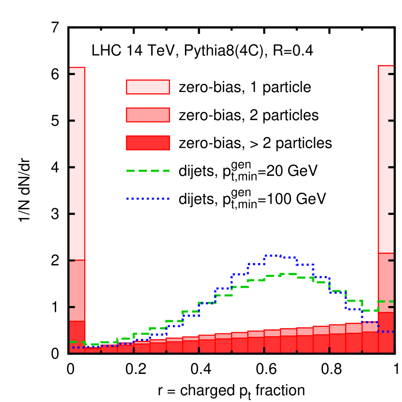
Figure 2: The filled histogram shows the distribution, for simulated zero-bias collisions, of the fraction, $r$, of the transverse momentum in a central circular patch of radius $R=0.4$ that is due to charged particles. It is separated into components according to the multiplicity of particles in the patch. The dashed and dotted histograms show the corresponding charged-fraction distributions for each of the two hardest anti-$k_{t}$, $R=0.4$ jets in simulated dijet events, with two choices for the hard generation cut $p_{t,\min}^{\text{gen}}$.

This point is illustrated in Fig. 2. We consider zero-bias events and examine a circular patch of radius $R=0.4$ centred at $y=\phi=0$. The figure shows the distribution of the charged $p_{t}$ fraction, $r$,

$$r=\frac{p_{t}^{\text{chg}}}{p_{t}^{\text{chg}+\text{ntr}}}\,,$$ (6)

in the patch (filled histogram, broken into contributions where the patch contains $1$, $2$ or more particles). The same plot also shows the distribution of the charged $p_{t}$ fraction in each of the two leading anti-$k_{t}$, $R=0.4$ jets in dijet events (dashed and dotted histograms). Whereas the charged-to-total ratio for a jet has a distribution peaked around $0.6$, as one would expect, albeit with a broad distribution, the result for zero-bias events is striking: in about 60% of events the patch is either just charged or just neutral, quite often consisting of just a single particle (weighting by the $p_{t}$ flow in the patch, the figure goes down to 30%). This is probably part of the reason why charged information provides only limited local information about neutral energy flow in pileup events.

These considerations are confirmed by an analysis of the actual performance of NpC and area–median subtraction. We reconstruct jets using the anti-$k_{t}$ algorithm [19], as implemented in FastJet [20], with a jet radius parameter of $R=0.4$. We study dijet and pileup events generated with Pythia 8.176 [21], in tune 4C; we assume idealised CHS, treating the charged pileup particles as ghosts. In the dijet (“hard”) event alone, i.e. without pileup, we run the jet algorithm and identify jets with absolute rapidity $|y|<2.5$ and transverse momentum $p_{t}>150\,\text{GeV}$. Then in the event with superposed pileup (the “full” event) we rerun the jet algorithm and identify the jets that match those selected in the hard event and subtract them using either NpC, Eq. (3), or the area–median method, Eq. (4), with $\rho$ estimated from the CHS event. The hard events are generated with the underlying event turned off, which enables us to avoid subtleties related to the simultaneous subtraction of the underlying event.

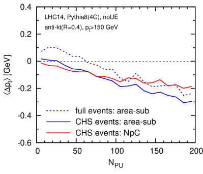
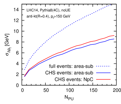
Figure 3: A comparison of the performance of the NpC and area–median subtraction methods. The left-hand plot shows, as a function of the number of pileup vertices $N_{\text{PU}}$, the average difference in $p_{t}$ between a jet after pileup addition and subtraction and the corresponding matched jet in the hard sample, $\Delta p_{t}=p_{t}^{\rm jet,sub}-p_{t}^{\rm jet,hard}$. The right-hand plot shows the standard deviation of $\Delta p_{t}$ (lower values are better). NpC is shown only for CHS events, while area–median subtraction is shown both for events with CHS and for events without it (“full”).

Figure 3 provides the resulting comparison of the performance of the NpC and area–median subtraction methods (the latter in CHS and in full events). The left-hand plot shows the average difference between the subtracted jet $p_{t}$ and the $p_{t}$ of the corresponding matched hard jet, as a function of the number of pileup interactions. Both methods clearly perform well here, with the average difference systematically well below $1\,\text{GeV}$ even for very high pileup levels. The right-hand plot shows the standard deviation of the difference between the hard and subtracted full jet $p_{t}$. A lower value indicates better performance, and one sees that in CHS events the area–median method indeed appears to have a small, but consistent advantage over NpC. Comparing area–median subtraction in CHS and full events, one observes a significant degradation in resolution when one fails to use the available information about charged particles in correcting the charged component of pileup, as is to be expected for a particle-level study.

The conclusion of this section is that the NpC method fails to give a superior performance to the area–median method in CHS events. This is because the local correlations of neutral and charged energy flow are no greater than the correlations between local neutral energy flow and the global energy flow. We believe that part of the reason for this is that the hadronisation process for low $p_{t}$ particles intrinsically tends to produce hadrons separated by large angles, as illustrated concretely in the case of $\rho^{\pm}$ resonance decay.

3 Cleansing

Part of the original motivation for our work here was to cross check a method recently introduced by Krohn, Low, Schwartz and Wang (KLSW) and called jet cleansing [9]. Cleansing comes in several variants. We will concentrate on linear cleansing, which was seen to perform well across a variety of observables by KLSW. It involves several elements: it breaks a jet into multiple subjets, as done for grooming methods like filtering and trimming [15, 14] (cf. also the early work by Seymour [22]). In its “linear” variant, it then corrects individual subjets for pileup by a method that is essentially the same as the NpC approach described in the previous section. Cleansing may also be used in conjunction with trimming-style cuts to the subtracted subjets, specifically it can remove those whose corrected transverse momentum is less than some fraction $f_{\text{cut}}$ of the overall jet’s transverse momentum (as evaluated before pileup removal).

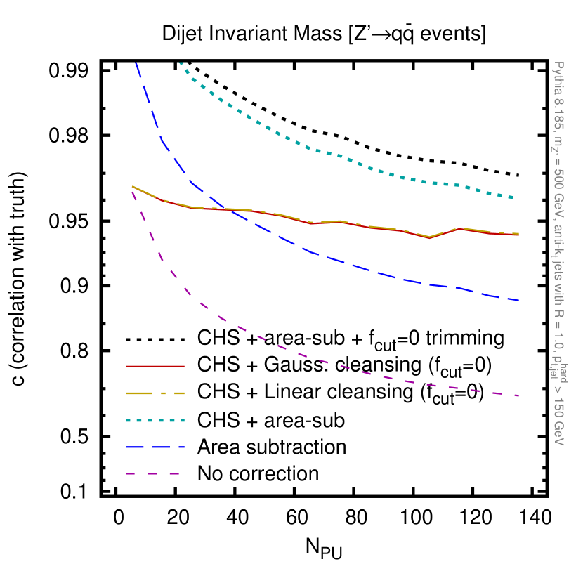
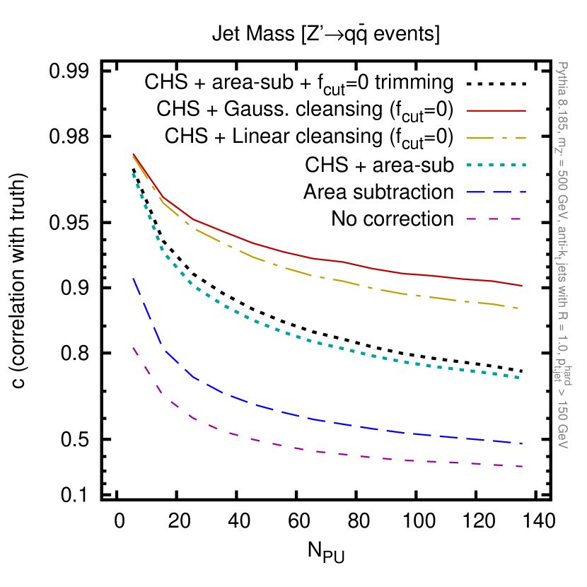
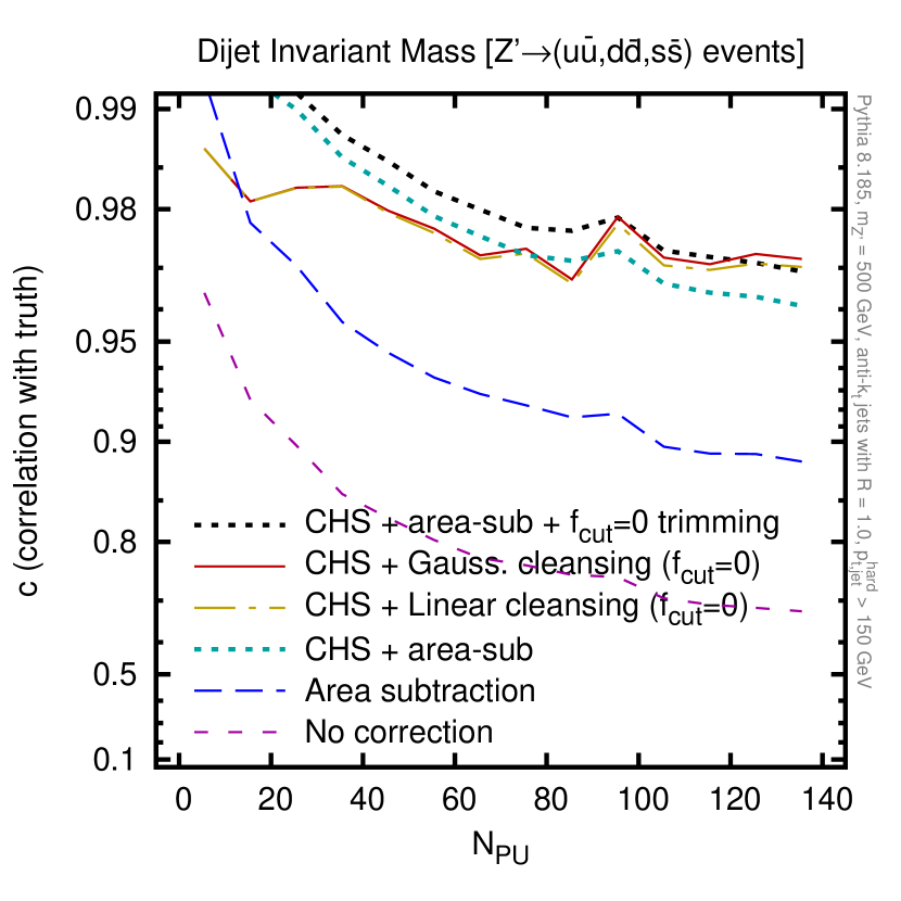
Figure 4: Upper left plot: the correlation coefficient between the dijet mass in hard events and the dijet mass after adding pileup and applying various pileup-removal methods; shown as a function of the number of pileup events, $N_{\text{PU}}$. Upper right plot: similarly for the single jet mass. Both plots are for a hadronically decaying $Z^{\prime}$ sample with $m_{Z^{\prime}}=500\,\text{GeV}$. Decays are included to all flavours except $t\bar{t}$ and $B$-hadrons are taken stable. Lower-left plot: the correlation coefficient for the dijet-mass, as in the upper-left plot, but with a sample of $Z^{\prime}$ bosons that decay only to $u$, $d$ and $s$ quarks. Jets are reconstructed, as in Ref. [9], with the anti-$k_{t}$ algorithm with $R=1$. For both trimming and cleansing, subjets are reconstructed with the $k_{t}$ algorithm with $R_{\text{sub}}=0.3$ and the $f_{\text{cut}}$ value that is applied is $f_{\text{cut}}=0$.

The top left-hand plot of Fig. 4 shows the correlation coefficient between the dijet mass in a hard event and the dijet mass after addition of pileup and application of each of several pileup mitigation methods. The results are shown as a function of $N_{\text{PU}}$. The pileup mitigation methods include two forms of cleansing (with $f_{\text{cut}}=0$), area–median subtraction, CHS+area subtraction, and CHS+area subtraction in conjunction with trimming (also with $f_{\text{cut}}=0$). The top right-hand plots shows the corresponding results for the jet mass. For the dijet mass we see that linear (and Gaussian) cleansing performs worse than area subtraction, while in the right-hand plot, for the jet mass, we see linear (and Gaussian) cleansing performing better than area subtraction, albeit not to the extent found in Ref. [9]. These (and, unless explicitly stated, our other $Z^{\prime}$ results) have been generated with the $Z^{\prime}$ decaying to all flavours except $t\bar{t}$, and $B$-hadrons have been kept stable. The lower plot shows the dijet mass for a different $Z^{\prime}$ sample, one that decays only to $u$, $d$ and $s$ quarks, but not $c$ and $b$ quarks. Most of the results are essentially unchanged. The exception is cleansing, which turns out to be very sensitive to the sample choice. Without stable $B$-hadrons in the sample, its performance improves noticeably and at high pileup becomes comparable to that of area-subtraction. Both of the left-hand plots in our Fig. 4 differ noticeably from Fig. 4 (left) of Ref. [9] and in particular they are not consistent with KLSW’s observation of much improved correlation coefficients for the dijet mass with cleansing relative to area+CHS subtraction.

Given our results on NpC in section 2, we were puzzled by the difference between the performance of area-subtraction plus trimming versus that of cleansing: our expectation is that their performances should be very similar. The strong sample-dependence of the cleansing performance also calls for an explanation. We thus continued our study of the question.

According to the description in Ref. [9], one additional characteristic of linear cleansing relative to area-subtraction is that it switches to jet-vertex-fraction (JVF) cleansing when the NpC-style rescaling would give a negative answer. In contrast, area-subtraction plus trimming simply sets the (sub)jet momentum to zero. We explicitly tried turning the switch to JVF-cleansing on and off and found it had a small effect and did not explain the differences.

Study of the public code for jet cleansing reveals an additional condition being applied to subjets: if a subjet contains no charged particles from the leading vertex (LV), then its momentum is set to zero. This step appears not to have been mentioned in Ref. [9]. Since we will be discussing it extensively, we find it useful to give it a name, “zeroing”. Zeroing can be thought of as an extreme limit of the charged-track based trimming procedure introduced by ATLAS [11], whereby a JVF-style cut is applied to reject subjets whose charged-momentum fraction from the leading vertex is too low. Zeroing turns out to be crucial: if we use it in conjunction with CHS area-subtraction (or with NpC subtraction) and $f_{\text{cut}}=0$ trimming, we obtain results that are very similar to those from cleansing. Conversely, if we turn this step off in linear-cleansing, its results come into accord with those from (CHS) area-subtraction or NpC-subtraction with $f_{\text{cut}}=0$ trimming.

To help illustrate this, Fig. 5 shows a “fingerprint” for each of several pileup-removal methods, for both the jet $p_{t}$ (left) and mass (right). The fingerprint includes the average shift ($\langle\Delta p_{t}\rangle$ or $\langle\Delta m\rangle$) of the observable after pileup removal, shown in black. It also includes two measures of the width of the $\Delta p_{t}$ and $\Delta m$ distributions: the dispersion (i.e. standard deviation) in red and an alternative peak-width measure in blue. The latter is defined as follows: one determines the width of the smallest window that contains $90\%$ of entries and then scales this width by a factor $0.304$. For a Gaussian distribution, the rescaling ensures that the resulting peak-width measure is equal to the dispersion. For a non-Gaussian distribution the two measures usually differ and the orange shaded region quantifies the extent of this difference. The solid black, blue and red lines have been obtained from samples in which the $Z^{\prime}$ decays just to light quarks; the dotted lines are for a sample including $c\bar{c}$ and $b\bar{b}$ decays (with stable $B$-hadrons), providing an indication of the sample dependence; in many cases they are indistinguishable from the solid lines.

Comparing $f_{\text{cut}}=0$ grooming for NpC, area (without zeroing) and cleansing with zeroing manually disabled, all have very similar fingerprints. Turning on zeroing in the different methods leads to a significant change in the fingerprints, but again NpC, area and cleansing are very similar.

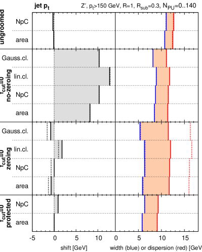
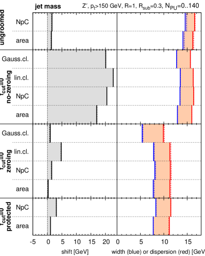
Figure 5: The left-hand plot illustrates various characteristics of the change ($\Delta p_{t}$) in the jet $p_{t}$ after addition of pileup and removal by a range of methods. It shows the average shift $\langle\Delta p_{t}\rangle$ (in black) and the peak width (in blue) and dispersion (in red) of the $\Delta p_{t}$ distribution. The peak width is defined as the smallest window of $\Delta p_{t}$ that contains 90% of the $\Delta p_{t}$ distribution, scaled by a factor $\simeq 0.304$ such that in the case of a Gaussian distribution the result agrees with the dispersion. The right-hand plot shows the same set of results for the jet mass. The results are obtained in a sample of events with the number of pileup vertices distributed uniformly between $0$ and $140$. The hard events consist of hadronic $Z^{\prime}$ decays: for the solid vertical lines the sample is $Z^{\prime}\to d\bar{d},u\bar{u},s\bar{s}$, while for the dotted lines (sometimes not visible because directly over the solid lines), the sample additionally includes $Z^{\prime}\to c\bar{c},b\bar{b}$ with $B$ hadrons kept stable. The $Z^{\prime}$ mass is $m_{Z^{\prime}}=500\,\text{GeV}$ and jets are reconstructed with the anti-$k_{t}$ algorithm with $R=1$. All results in this figure include charged-hadron subtraction by default. The default form of cleansing, as used e.g. in Fig. 4, is “$f_{\text{cut}}=0$ zeroing”.

When used with $f_{\text{cut}}=0$ trimming, and when examining quality measures such as the dispersion (in red, or the closely related correlation coefficient, cf. Appendix B), subjet zeroing appears to be advantageous for the jet mass, but potentially problematic for the jet $p_{t}$ and the dijet mass. However, the dispersion quality measure does not tell the full story regarding the impact of zeroing. Examining simultaneously the peak-width measure (in blue) makes it easier to disentangle two different effects of zeroing. On one hand we find that zeroing correctly rejects subjets that are entirely due to fluctuations of the pileup. This narrows the peak of the $\Delta p_{t}$ or $\Delta m$ distribution, substantially reducing the (blue) peak-width measures in Fig. 5. On the other hand, zeroing sometimes incorrectly rejects subjets that have no charged tracks from the LV but do have significant neutral energy flow from the LV. This can lead to long tails for the $\Delta p_{t}$ or $\Delta m$ distributions, adversely affecting the dispersion. It is the interplay between the narrower peak and the longer tails that affects whether overall the dispersion goes up or down with zeroing. In particular the tails appear to matter more for the jet $p_{t}$ and dijet mass than they do for the single-jet mass. Note that accurate Monte Carlo simulation of such tails may be quite challenging: they appear to be associated with configurations where a subjet contains an unusually small number of energetic neutral particles. Such configurations are similar to those that give rise to fake isolated photons or leptons and that are widely known to be difficult to simulate correctly.

We commented earlier that the cleansing performance has a significant sample dependence. This is directly related to the zeroing: indeed Fig. 5 shows that for cleansing without zeroing, the sample dependence (dashed versus solid lines) vanishes, while it is substantial with zeroing. Our understanding of this feature is that the lower multiplicity of jets with undecayed $B$-hadrons (and related hard fragmentation of the $B$-hadron) results in a higher likelihood that a subjet will contain neutral but no charged particles from the LV, thus enhancing the impact of zeroing on the tail of the $\Delta p_{t}$ or $\Delta m_{jj}$ sample.

The long tails produced by the zeroing are not necessarily unavoidable. In particular, they can correspond to the loss of subjets with tens of GeV, yet it is very unlikely that a subjet from a pileup collision will be responsible for such a large energy. Therefore we introduce a modified procedure that we call “protected zeroing”: one rejects any subjet without LV tracks unless its $p_{t}$ after subtraction is $n$ times larger than the largest charged $p_{t}$ in the subjet from any single pileup vertex (or, more simply, just above some threshold $p_{t,\text{min}}$; however, using $n$ times the largest charged subjet $p_{t}$ could arguably be better both in cases where one explores a wide range of $N_{\text{PU}}$ and for situations involving a hard subjet from a pileup collision). Taking $n=10$ (or a fixed $p_{t,\text{min}}=20\,\text{GeV}$) we have found reduced tails and, consequently, noticeable improvements in the jet $p_{t}$ and dijet mass dispersion (with little effect for the jet mass). This is visible for area and NpC subtraction in Fig. 5. Protected zeroing also eliminates the sample dependence.

Several additional comments can be made about $f_{\text{cut}}=0$ trimming combined with zeroing. Firstly, $f_{\text{cut}}=0$ trimming alone introduces a bias in the jet $p_{t}$, which is clearly visible in the $f_{\text{cut}}=0$ no-zeroing shifts in Fig. 5. This is because the trimming removes negative fluctuations of the pileup, but keeps the positive fluctuations. Zeroing then counteracts that bias by removing some of the positive fluctuations, those that happened not to have any charged tracks from the LV. It also introduces further negative fluctuations for subjets that happened to have some neutral energy flow but no charged tracks. Overall, one sees that the final net bias comes out to be relatively small. This kind of cancellation between different biases is common in noise-reducing pileup-reduction approaches [26, 27, 28].

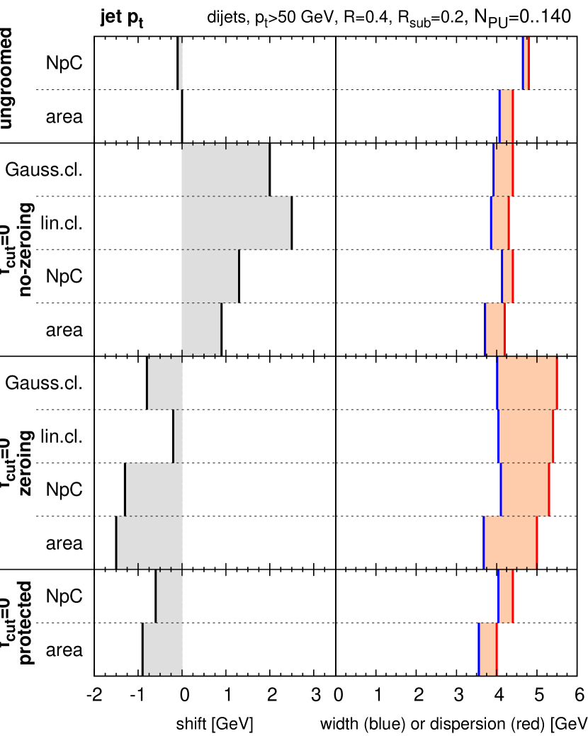
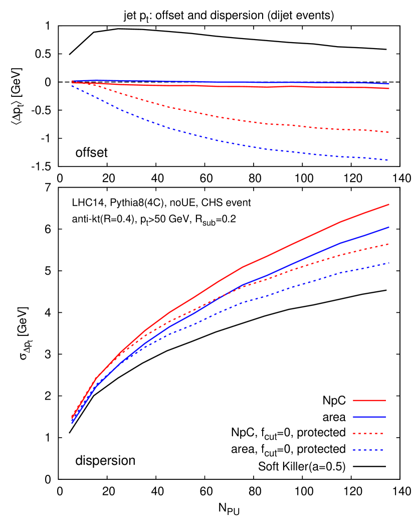
Figure 6: Left, Analogue of Fig. 5 (left) for a jet radius of $R=0.4$, subjet radius (where relevant) of $R_{\text{sub}}=0.2$ and a QCD continuum dijet sample generated with Pythia 8. The underlying event is turned off in the sample and $B$ hadrons decay. We consider only jets that in the hard sample have $p_{t}>50\,\text{GeV}$ and $|y|<2.5$. Right: the dispersions for a subset of the methods, shown as a function of the number of pileup events.

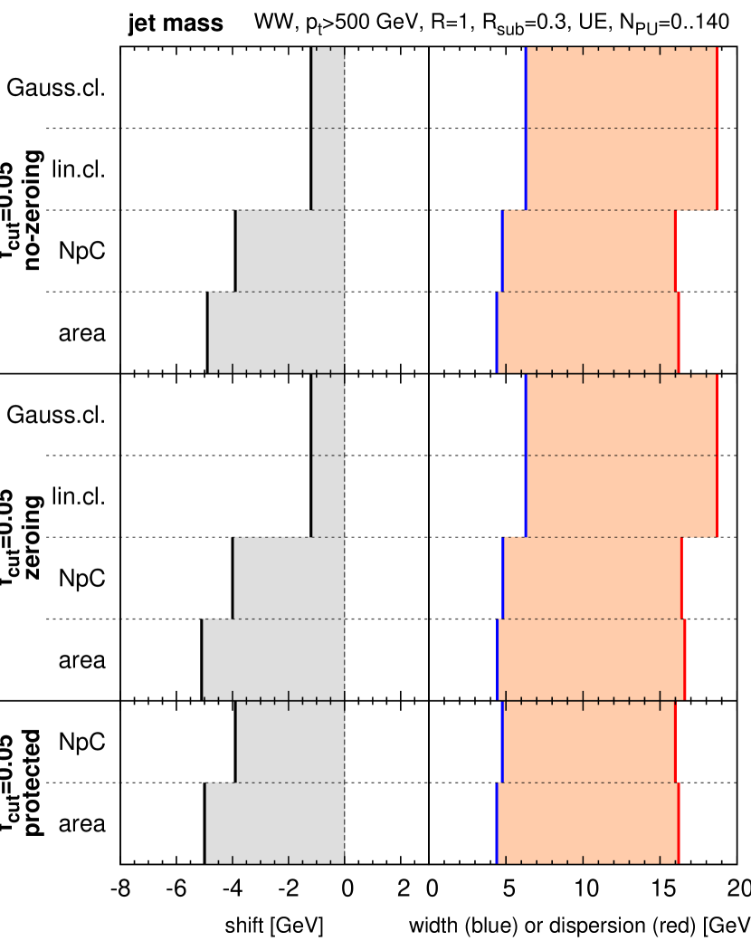
Figure 7: Analogue of Fig. 5 (right), showing the performance for the jet mass, but now with $f_{\text{cut}}=0.05$ applied to both trimming and cleansing and in a sample of hadronically-decaying boosted $W$ bosons ($pp\to W^{+}W^{-}$). The jets reconstructed after addition and subtraction of pileup are compared to trimmed hard jets. Jets are reconstructed with a jet radius of $R=1$ and a subjet radius of $R_{\text{sub}}=0.3$. Only hard jets with $p_{t}>500\,\text{GeV}$ and $|y|<2.5$ (before trimming) are considered and we let $B$ hadrons decay.

Most of the studies so far in this section have been carried out with a setup that is similar to that of Ref. [9], i.e. $R=1$ jets in a $Z^{\prime}$ sample with $f_{\text{cut}}=0$ trimming. This is not a common setup for most practical applications. For most uses of jets, $R=0.4$ is a standard choice and pileup is at its most severe at low to moderate $p_{t}$. Accordingly, in Fig. 6 (left) we show the analogue of Fig. 5’s summary for the jet $p_{t}$, but now for $R=0.4$, with $R_{\text{sub}}=0.2$ in a QCD dijet sample, considering jets that in the hard event had $p_{t}>50\,\text{GeV}$. We see that qualitatively the pattern is quite similar to that in Fig. 5. Quantitatively, the difference between the various choices is much smaller, with about a $10\%$ reduction in dispersion (or width) in going from ungroomed CHS area-subtraction to the $f_{\text{cut}}=0$ protected subjet-zeroing case. One should be aware that this study is only for a single $p_{t}$, across a broad range of pileup. The dispersions for a subset of the methods are shown as a function of the number of pileup vertices in the right-hand plot of Fig. 6. That plot also includes results from the SoftKiller method [27] and illustrates that the benefit from protected zeroing (comparing the solid and dashed blue curves) is about half of the benefit that is brought from SoftKiller (comparing solid blue and black curves). These plots show that protected zeroing is potentially of interest for jet $p_{t}$ determinations in realistic conditions. Thus it would probably benefit from further study: one should, for example, check its behaviour across a range of transverse momenta, determine optimal choices for the protection of the zeroing and investigate also how best to combine it with particle-level subtraction methods such as SoftKiller.

Turning now to jet masses, the use of $R=1$ is a not uncommon choice, however most applications use a groomed jet mass with a non-zero $f_{\text{cut}}$ (or its equivalent): this improves mass resolution in the hard event even without pileup, and it also reduces backgrounds, changing the perturbative structure of the jet [29, 30] even in the absence of pileup. Accordingly in Fig. 7 we show $f_{\text{cut}}=0.05$ results (with shifts and widths computed relative to $f_{\text{cut}}=0.05$ trimmed hard jets) for a hard $WW$ sample where the hard fat jets are required to have $p_{t}>500\,\text{GeV}$. Zeroing, whether protected or not, appears to have little impact. One potential explanation for this fact is as follows: zeroing’s benefit comes primarily because it rejects fairly low-$p_{t}$ pileup subjets that happen to have no charged particles from the leading vertex. However for a pileup subjet to pass the $f_{\text{cut}}=0.05$ filtering criterion in our sample, it would have to have $p_{t}>25\,\text{GeV}$. This is quite rare. Thus filtering is already removing the pileup subjets, with little further to be gained from the charged-based zeroing. As in the plain jet-mass summary plot, protection of zeroing appears to have little impact for the trimmed jet mass. Does that mean that (protected) zeroing has no scope for improving the trimmed-jet mass? The answer is “not necessarily”: one could for example imagine first applying protected zeroing to subjets on some angular scale $R_{\text{zero}}$ in order to eliminate low-$p_{t}$ contamination; then reclustering the remaining constituents on a scale $R_{\text{trim}}\gtrsim R_{\text{zero}}$, subtracting according to the area or NpC methods, and finally applying the trimming momentum cut (while also keeping in mind the considerations of footnote 21).

We close this section with a summary of our findings. Based on its description in Ref. [9] and our findings about NpC v. area subtraction, cleansing with $f_{\text{cut}}=0$ would be expected to have a performance very similar to that of CHS+area subtraction with $f_{\text{cut}}=0$ trimming. Ref. [9] however reported large improvements for the correlation coefficients of the dijet mass and the single jet mass using $R=1$ jets. In the case of the dijet mass we do not see these improvements, though they do appear to be there for the jet mass. The differences in behaviour between cleansing and trimmed CHS+area-subtraction call for an explanation, and appear to be due to a step in the cleansing code that was undocumented in Ref. [9] and that we dubbed “zeroing”: if a subjet contains no charged tracks from the leading vertex it is discarded. Zeroing is an extreme form of a procedure described in Ref. [11]. In can be used also with area or NpC subtraction, and we find that it brings a benefit for the peak of the $\Delta p_{t}$ and $\Delta m$ distributions, but appears to introduce long tails in $\Delta p_{t}$. A variant, “protected zeroing”, can avoid the long tails by still accepting subjets without leading-vertex tracks, if their $p_{t}$ is above some threshold, which may be chosen dynamically based on the properties of the pileup. In our opinion, a phenomenologicaly realistic estimate of the benefit of zeroing (protected or not) requires study not of $R=1$ plain jets, but instead of $R=0.4$ jets (for the jet $p_{t}$) or larger-$R$ trimmed jets with a non-zero $f_{\text{cut}}$ (for the jet mass). In a first investigation, there appear to be some phenomenological benefits from protected zeroing for the $R=0.4$ jet $p_{t}$, whereas to obtain benefits for large-$R$ trimmed jets would probably require further adaptation of the procedure. In any case, additional study is required for a full evaluation of protected zeroing and related procedures.

4 Combining NpC and area subtraction

It is interesting to further probe the relation between NpC and the area–median method, to establish whether there might be a benefit from combining them: the area–median method makes a mistake in predicting local energy flow mainly because local energy flow fluctuates from region to region. NpC makes a mistake because charged and neutral energy flow are not $100\%$ locally correlated. The key question is whether, for a given jet, NpC and the area–median method generally make the same mistake, or if instead they are making uncorrelated mistakes. In the latter case it should be possible to combine the information from the two methods to obtain an improvement in subtraction performance.

Let $p_{t}^{\text{ntr}}$ be the actual neutral pileup component flowing into a jet, while

$$\hat{p}_{\mu}^{\text{ntr(NpC)}}=\frac{1-\gamma_{0}}{\gamma_{0}\epsilon}p_{\mu}^{\text{jet,rescaled-chg-PU}}\,,\qquad\hat{p}_{\mu}^{\text{ntr($\rho A$)}}=\rho A\,,$$ (7)

are, respectively, the estimates for the neutral pileup based on the local charged $p_{t}$ flow and on $\rho A$. We assume the use of CHS events and, in particular, that $\rho$ is as determined from the CHS event. Concentrating on the transverse components, the extent to which the two estimates provide complementary information can be quantified in terms of (one minus) the correlation coefficient, $r$, between $p_{t}^{\text{ntr}}-\hat{p}_{\mu}^{\text{ntr(NpC)}}$ and $p_{t}^{\text{ntr}}-\hat{p}_{\mu}^{\text{ntr($\rho A$)}}$. That correlation is shown as a function of $R$ in Fig. 8 (left), and it is quite high, in the range $0.6$–$0.7$ for commonly used $R$ choices. It is largely independent of the number of pileup vertices.

Let us now quantify the gain to be had from a linear combination of the two prediction methods, i.e. using an estimate

$$\hat{p}_{\mu}^{\text{ntr}}=f\hat{p}_{\mu}^{\text{ntr(NpC)}}+(1-f)\hat{p}_{\mu}^{\text{ntr($\rho A$)}}\,,$$ (8)

where $f$ is to be chosen to as to minimise the dispersion of $p_{t}^{\text{ntr}}-\hat{p}_{t}^{\text{ntr}}$. Given dispersions $\sigma_{\text{NpC}}$ and $\sigma_{\rho A}$ respectively for $p_{t}^{\text{ntr}}-\hat{p}_{\mu}^{\text{ntr(NpC)}}$ and $p_{t}^{\text{ntr}}-\hat{p}_{\mu}^{\text{ntr($\rho A$)}}$, the optimal $f$ is

$$f=\frac{\sigma_{\rho A}^{2}-r\,\sigma_{\text{NpC}}\,\sigma_{\rho A}}{\sigma_{\text{NpC}}^{2}+\sigma_{\rho A}^{2}-2r\,\sigma_{\text{NpC}}\,\sigma_{\rho A}}\,,$$ (9)

which is plotted as a function of $R$ in Fig. 8 (right), and the resulting squared dispersion for $p_{t}^{\text{ntr}}-\hat{p}_{t}^{\text{ntr}}$ is

$$\sigma^{2}=\frac{(1-r^{2})\,\sigma_{\text{NpC}}^{2}\,\sigma_{\rho A}^{2}}{\sigma_{\text{NpC}}^{2}+\sigma_{\text{ntr}}^{2}-2r\,\sigma_{\text{NpC}}\,\sigma_{\rho A}}\,.$$ (10)

Reading $r=0.67$ from Fig. 8 (left) for $R=0.4$, and $\sigma_{\text{NpC}}\simeq 1.14\,\sigma_{\rho A}$ from Fig. 1 (right), one finds $\sigma\simeq 0.96\,\sigma_{\rho A}$. Because of the substantial correlation between the two methods, ones expects only a modest gain from their linear combination.

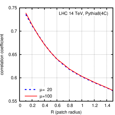
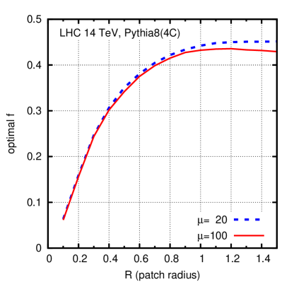
Figure 8: Left: correlation between $p_{t}^{\text{ntr}}-\hat{p}_{\mu}^{\text{ntr(NpC)}}$ and $p_{t}^{\text{ntr}}-\hat{p}_{\mu}^{\text{ntr($\rho A$)}}$, shown as a function of $R$. Right: optimal weight $f$ for combining NpC and area pileup subtraction, Eq. (9), as a function of $R$.

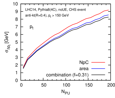
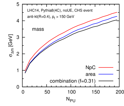
Figure 9: Comparison of the performance of NpC, area–median and combined subtraction, as a function of the number of pileup vertices. The left-hand plot is for the jet $p_{t}$ and the right-hand one for the jet mass.

In Fig. 9 we compare the performance of pileup subtraction from the combination of the NpC and the area–median methods, using the optimal value $f=0.31$ that can be read from Fig. 8 (right) for $R=0.4$, both for the jet $p_{t}$ and the jet mass. The expected small gain is indeed observed for the jet $p_{t}$, and it is slightly larger for the jet mass. Given the modest size of the gain, one may wonder how phenomenologically relevant it is likely to be. Nevertheless, one might still consider investigating whether the gain carries over also to a realistic experimental environment with full detector effects.

5 Conclusions

One natural approach to pileup removal is to use the charged pileup particles in a given jet to estimate the amount of neutral pileup that needs to be removed from that same jet. In this article, with the help of particle-level simulations, we have studied such a method (NpC) and found that it has a performance that is similar to, though slightly worse than the existing, widely used area–median method. This can be related to the observation that the correlations between local charged and neutral energy flow are no larger than those between global and local energy flow. Tentatively, we believe that this is in part because the non-perturbative effects that characterise typical inelastic proton-proton collisions act to destroy local charged-neutral correlation.

The absence of benefit that we found from the NpC method led us to question the substantial performance gains quoted for the method of cleansing in Ref. [9], one of whose key differences with respect to earlier work is the replacement of the area–median method with NpC. For the dijet mass, we are unable to reproduce the large improvement observed in Ref. [9], in the correlation coefficient performance measure, for cleansing relative to area subtraction. We do however see an improvement for the jet mass. We trace a key difference in the behaviour of cleansing and area subtraction to the use in the cleansing code of a step that was not documented in Ref. [9] and that discards subjets that contain no tracks from the leading vertex. This “zeroing” step, similar to the charged-track based trimming introduced by ATLAS [11], can indeed be of benefit. It has a drawback of introducing tails in some distributions due to subjets with a substantial neutral $p_{t}$ from the leading vertex, but no charged tracks. As a result, different quality measures lead to different conclusions as to the benefits of zeroing. The tails can be alleviated by a variant of zeroing that we introduce here, “protected zeroing”, whereby subjets without LV charged tracks are rejected only if their $p_{t}$ is below some (possibly pileup-dependent) threshold. Protected zeroing does in some cases appear to have phenomenological benefits, which are observed across all quality measures.

Given two different methods for pileup removal, NpC and area–median subtraction, it is natural to ask how independent they are and what benefit might be had by combining them. This was the question investigated in section 4, where we provided a formula for an optimal linear combination of the two methods, as a function of their degree of correlation. Ultimately we found that NpC and area–median subtraction are quite highly correlated, which limits the gains from their combination to about a $5\%$ percent reduction in dispersion. While modest, this might still be sufficient to warrant experimental investigation, as are other methods, currently being developed, that exploit constituent-level subtraction [31, 32, 27, 28]. A study of the integration of those methods with protected zeroing would also be of interest.

Code for our implementation of area subtraction with positive-definite mass is available as part of FastJet versions 3.1.0 and higher. Public code and samples for carrying out a subset of the comparisons with cleansing described in section 3, including also the NpC subtraction tools, are available from Ref. [36].

Appendix A Details of our study

Let us first fully specify what we have done in our study and then comment on (possible) differences relative to KLSW.

Our hard event sample consists of dijet events from $pp$ collisions at $\sqrt{s}=14\,\text{TeV}$, simulated with Pythia 8.176 [21], tune 4C, with a minimum $p_{t}$ in the $2\to 2$ scattering of $135\,\text{GeV}$ and with the underlying event turned off, except for the plots presented in Figs. 4 and 5, where we use $Z^{\prime}$ events with $m_{Z^{\prime}}=500\,\text{GeV}$. Jets are reconstructed with the anti-$k_{t}$ algorithm [19] after making all particles massless (preserving their rapidity) and keeping only particles with $|y|<4$. We have $R=0.4$, except for the some of the results presented in Section 3 and Appendix B, where we use $R=1$ as in Ref. [9].

Given a hard event, we select all the jets with $p_{t}>150\,\text{GeV}$ and absolute rapidity $|y|<2.5$. We then add pileup and cluster the resulting full event, i.e. including both the hard event and the pileup particles, without imposing any $p_{t}$ or rapidity cut on the resulting jets. For each jet selected in the hard event as described above, we find the jet in the full event that overlaps the most with it. Here, the overlap is defined as the scalar $p_{t}$ sum of all the common jet constituents, as described in footnote 8 on p. 8. Given a pair of jets, one in the hard event and the matching one in the full event, we can apply subtraction/grooming/cleansing to the latter and study the quality of the jet $p_{t}$ or jet mass reconstruction. For studies involving the dijet mass (cf. Fig. 4) we require that at least two jets pass the jet selection in the hard event and use those two hardest jets, and the corresponding matched ones in the full event, to reconstruct the dijet mass. This approach avoids having to additionally consider the impact of pileup on the efficiency for jet selection, which cannot straightforwardly be folded into our quality measures.

Most of the studies shown in this paper use idealised particle-level CHS events. In these events, we scale all charged pileup hadrons by a factor $\epsilon=10^{-60}$ before clustering, to ensure that they do not induce any backreaction [4]. The jet selection and matching procedures are independent of the use of CHS or full events. When we plot results as a function of the quantity $N_{\text{PU}}$, this corresponds to the actual (fixed) number of zero-bias events superimposed onto the hard collision. For results shown as a function of $\mu$, the average number of zero-bias events, the actual number of zero-bias events has a Poisson distribution. Clustering and area determination are performed with a development version of FastJet 3.1 (which for the features used here behaves identically to the 3.0.x series) and with FastJet 3.1.0 and 3.1.1 for the results in section 3.

Details of how the area-median subtraction is performed could conceivably matter. Jet areas are obtained using active area with explicit ghosts placed up to $|y|=4$ and with a default ghost area of 0.01. We use FastJet’s GridMedianBackgroundEstimator with a grid spacing of 0.55 to estimate the event background density $\rho$. The $\rho$ estimation is performed using the particles (up to $|y|=4$) from the full or the CHS event as appropriate. When subtracting pileup from jets, we account for the rapidity dependence of $\rho$, based on the rapidity dependence in a pure pileup sample (as discussed in Refs. [20, 35]). We carry out 4-vector subtraction $p_{\mu}^{\text{sub}}=p_{\mu}-A_{\mu}\rho(y_{\text{jet}})$.

A few obviously unphysical situations need special care. For jets obtained from the full event, if $A_{t}\rho>p_{t}^{\text{jet}}$, we set $p_{\mu}^{\text{sub}}$ to a vector with zero transverse momentum, zero mass, and the rapidity and azimuth of the original unsubtracted jet; and if $(p^{\text{sub}})^{2}$ is negative, an unphysical situation since it would lead to an imaginary mass, we replace $p_{\mu}^{\text{sub}}$ with a vector with the same transverse components, zero mass, and the rapidity of the original unsubtracted jet. This is essentially equivalent to replacing negative squared masses with zero.

The case of CHS events is a bit more delicate. Let $p_{\mu}^{\text{chg}}$ denote the 4-momentum of the charged component of the jet. Then, if $p_{t}^{\text{sub}}<p_{t}^{\text{chg}}$, we set $p_{\mu}^{\text{sub}}=p^{\text{chg}}_{\mu}$, and when $(p^{\text{sub}})^{2}<(p^{\text{chg}})^{2}$, we replace $p_{\mu}^{\text{sub}}$ with a vector with the same transverse components, and the mass and rapidity of $p^{\text{chg}}_{\mu}$. For jets with no charged component, whenever the resulting 4-vector has an ill-defined rapidity or azimuthal angle, we use those of the original jet. Corresponding tests that the subtracted transverse momentum and mass are non-negative are also applied in our NpC subtraction. These safety requirements have little impact on the single-jet $p_{t}$, limited impact on the dijet mass, and for the single-jet mass improve the dispersion of the subtraction relative to the choice (widespread in computer codes) of taking $m\equiv-\sqrt{|m^{2}|}$ when $m^{2}<0$.

One difference between our study and KLSW’s is that we carry out a particle-level study, whereas they project their event onto a toy detector with a $0.1\times 0.1$ tower granularity, removing charged particles with $p_{t}<0.5\,\text{GeV}$ and placing a $1\,\text{GeV}$ threshold on towers. In our original (v1) studies with $f_{\text{cut}}=0.05$ we tried including a simple detector simulation along these lines and did not find any significant modification to the pattern of our results, though CHS+area subtraction is marginally closer to the cleansing curves in this case.

Cleansing has two options: one can give it jets clustered from the full event, and then it uses an analogue of Eq. (1): this effectively subtracts the exact charged part and the NpC estimate of the neutrals. Or one can give it jets clustered from CHS events, and it then applies the analogue of Eq. (3), which assumes that there is no charged pileup left in the jet and uses just the knowledge of the actual charged pileup to estimate (and subtract) the neutral pileup. These two approaches differ by contributions related to back-reaction. Our understanding is that KLSW took the former approach, while we used the latter. Specifically, our charged-pileup hadrons, which are scaled down in the CHS event, are scaled back up to their original $p_{t}$ before passing them to the cleansing code, in its input_nc_separate mode. If we use cleansing with full events, we find that its performance worsens, as is to be expected given the additional backreaction induced when clustering the full event. Were it not for backreaction, cleansing applied to full or CHS events should essentially be identical.

Regarding the NpC and cleansing parameters, our value of $\gamma_{0}=0.612$ differs slightly from that of KLSW’s $\gamma_{0}=0.55$, and corresponds to the actual fraction of charged pileup in our simulated events. In our tests with a detector simulation like that of KLSW, we adjusted $\gamma_{0}$ to its appropriate (slightly lower) value.

Finally, for trimming we use $R_{\rm trim}=0.3$ and the reference $p_{t}$ is taken unsubtracted, while the subjets are subtracted before performing the trimming cut, which removes subjets with $p_{t}$ below a fraction $f_{\text{cut}}$ times the reference $p_{t}$. Compared to using the subtracted $p_{t}$ as the reference for trimming, this effectively places a somewhat harder cut as pileup is increased. For comparisons with cleansing we generally use $f_{\text{cut}}=0$ unless explicitly indicated otherwise.

Appendix B The correlation coefficient as a quality measure

In this appendix, we discuss some characteristics of correlation coefficients that affect their appropriateness as generic quality measures for pileup studies.

Suppose we have an observable $v$. Define

$$\Delta v=v^{\text{sub}}-v^{\text{hard}}\,,$$ (11)

to be the difference, in a given event, between the pileup subtracted observable and the original “hard” value without pileup. Two widely used quality measures for the performance of pileup subtraction are the average offset of $v$, $\langle\Delta v\rangle$ and the standard deviation of $\Delta v$, which we write as $\sigma_{\Delta v}$. One might think there is a drawback in keeping track of two measures, in part because it is not clear which of the two is more important. It is our view that the two measures provide complementary information: if one aims to reduce systematic errors in a precision measurement then a near-zero average offset may be the most important requirement, so as not to be plagued by issues related to the systematic error on the offset. In a search for a resonance peak, then one aims for the narrowest peak, and so the smallest possible standard deviation.

The quality measure advocated in [9] is instead the correlation coefficient between $v^{\text{sub}}$ and $v^{\text{hard}}$. This has the apparent simplifying advantage of providing just a single quality measure. However, it comes at the expense of masking potentially important information: for example, a method with a large offset and one with no offset will give identical correlation coefficients, because the correlation coefficient is simply insensitive to (constant) offsets.

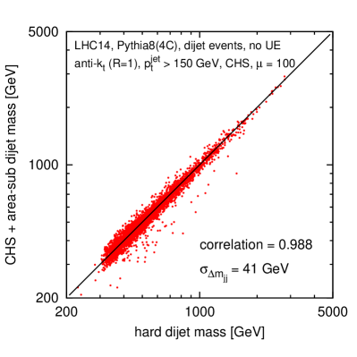
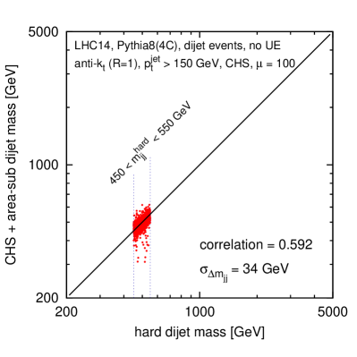
Figure 10: Left: scatter plot of the dijet mass after addition of an average of $100$ pileup events and area–median subtraction (in CHS events) versus the dijet mass in the original hard event. The hard dijet sample and the analysis are as described in appendix A, with a jet radius of $R=1$. The right-hand plot is identical except for the following additional condition on the hard event: $450<m_{jj}<550\,\text{GeV}$. Note the lower correlation coefficient, even though the lower $\sigma_{\Delta m_{jj}}$ suggests better typical subtraction in this specific mass bin.

The correlation coefficient has a second, more fundamental flaw, as illustrated in Fig. 10. On the left, one has a scatter plot of the dijet mass in PU-subtracted events versus the dijet mass in the corresponding hard events, as obtained in an inclusive jet sample. There is a broad spread of dijet masses, much wider than the standard deviation of $\Delta m_{jj}$, and so the correlation coefficient comes out very high, $c=0.988$. Now suppose we are interested in reconstructing resonances with a mass near $500\,\text{GeV}$, and so consider only hard events in which $450<m_{jj}<550\,\text{GeV}$ (right-hand plot). Now the correlation coefficient is $0.59$, i.e. much worse. This does not reflect a much worse subtraction: actually, $\sigma_{\Delta m_{jj}}$ is better (lower) in the sample with a limited $m_{jj}$ window, $\sigma_{\Delta m_{jj}}=34\,\text{GeV}$, than in the full sample, $\sigma_{\Delta m_{jj}}=41\,\text{GeV}$. The reason for the puzzling decrease in the correlation coefficient is that the dispersion of $m_{jj}$ is much smaller than before, and so the dispersion of $\Delta m_{jj}$ is now comparable to that of $m_{jj}$: it is this, and not an actual degradation of performance, that leads to a small correlation.

This can be understood quantitatively in a simple model with two variables: let $v^{\text{hard}}$ have a standard deviation of $\sigma_{v,\text{hard}}$, and for a given $v^{\text{hard}}$ let $v^{\text{sub}}$ be distributed with a mean value equal to $v^{\text{hard}}$ (plus an optional constant offset) and a standard deviation of $\sigma_{\Delta v}$ (independent of $v^{\text{hard}}$). Then the correlation coefficient of $v^{\text{hard}}$ and $v^{\text{sub}}$ is

$$c=\frac{\sigma_{v,\text{hard}}}{\sqrt{(\sigma_{v,\text{hard}})^{2}+\sigma_{\Delta v}^{2}}}\,,$$ (12)

i.e. it tends to zero for $\sigma_{v,\text{hard}}\ll\sigma_{\Delta v}$ and to $1$ for large $\sigma_{v,\text{hard}}\gg\sigma_{\Delta v}$, in accord with the qualitative behaviour seen in Fig. 10. The discussion becomes more involved if $\langle v^{\text{sub}}\rangle$ has a more complicated dependence on $v^{\text{hard}}$ or if $\sigma_{\Delta v}$ itself depends on $v^{\text{hard}}$, for example as is actually the case for the dijet mass with the analysis of Appendix A.

The main conclusion from this appendix is that correlation coefficients mix together information about the quality of pileup mitigation and information about the hard event sample being studied. It is then highly non-trivial to extract just the information about the pileup subtraction. This can lead to considerable confusion, for example, when evaluating the robustness of a method against the choice of hard sample. Overall therefore, it is our recommendation that one consider direct measures of the dispersion introduced by the pileup and subtraction and not correlation coefficients. In cases with severely non-Gaussian tails in the $\Delta v$ distributions it can additionally be useful to consider quality measures more directly related to the peak structure of the $\Delta v$ distribution.

References

- [1] The ATLAS collaboration, “Pile-up subtraction and suppression for jets in ATLAS,” ATLAS-CONF-2013-083.
- [2] CMS Collaboration, “Jet Energy Scale performance in 2011,” CMS-DP-2012-006.
- [3] M. Cacciari and G. P. Salam, Phys. Lett. B 659 (2008) 119 [arXiv:0707.1378 [hep-ph]].
- [4] M. Cacciari, G. P. Salam and G. Soyez, JHEP 0804 (2008) 005 [arXiv:0802.1188 [hep-ph]].
- [5] CMS Collaboration, “Particle-Flow Event Reconstruction in CMS and Performance for Jets, Taus, and MET,” CMS-PAS-PFT-09-001.
- [6] G. Aad et al. [ATLAS Collaboration], Phys. Lett. B 716 (2012) 1 [arXiv:1207.7214 [hep-ex]].
- [7] J. Colas et al. [ATLAS Liquid Argon Calorimeter Collaboration], Nucl. Instrum. Meth. A 550 (2005) 96 [physics/0505127].
- [8] M. Cacciari, G. P. Salam and G. Soyez, unpublished, presented at CMS Week, CERN, Geneva, Switzerland, March 2011, available publicly since then at http://www.lpthe.jussieu.fr/~salam/talks/repo/2011-CMS-week.pdf.
- [9] D. Krohn, M. D. Schwartz, M. Low and L. T. Wang, Phys. Rev. D 90 (2014) 6, 065020 [arXiv:1309.4777 [hep-ph]].
- [10] CMS Collaboration, “Pileup Jet Identification,” CMS-PAS-JME-13-005.
- [11] ATLAS Collaboration, “Tagging and suppression of pileup jets,” ATL-PHYS-PUB-2014-001.
- [12] M. Cacciari, J. Rojo, G. P. Salam and G. Soyez, JHEP 0812 (2008) 032 [arXiv:0810.1304 [hep-ph]].
- [13] A. Altheimer, A. Arce, L. Asquith, J. Backus Mayes, E. Bergeaas Kuutmann, J. Berger, D. Bjergaard and L. Bryngemark et al., arXiv:1311.2708 [hep-ex].
- [14] J. M. Butterworth, A. R. Davison, M. Rubin and G. P. Salam, Phys. Rev. Lett. 100 (2008) 242001 [arXiv:0802.2470 [hep-ph]].
- [15] D. Krohn, J. Thaler and L. -T. Wang, JHEP 1002 (2010) 084 [arXiv:0912.1342 [hep-ph]].
- [16] M. Cacciari, J. Rojo, G. P. Salam and G. Soyez, Eur. Phys. J. C 71 (2011) 1539 [arXiv:1010.1759 [hep-ph]].
- [17] G. Soyez, G. P. Salam, J. Kim, S. Dutta and M. Cacciari, Phys. Rev. Lett. 110 (2013) 16, 162001 [arXiv:1211.2811 [hep-ph]].
- [18] M. Cacciari, P. Quiroga-Arias, G. P. Salam and G. Soyez, Eur. Phys. J. C 73 (2013) 2319 [arXiv:1209.6086 [hep-ph]].
- [19] M. Cacciari, G. P. Salam and G. Soyez, JHEP 0804 (2008) 063 [arXiv:0802.1189 [hep-ph]].
- [20] M. Cacciari, G. P. Salam and G. Soyez, Eur. Phys. J. C 72 (2012) 1896 [arXiv:1111.6097 [hep-ph]].
- [21] T. Sjostrand, S. Mrenna and P. Z. Skands, Comput. Phys. Commun. 178 (2008) 852 [arXiv:0710.3820 [hep-ph]].
- [22] M. H. Seymour, Z. Phys. C 62 (1994) 127.
-
[23]
M. D. Schwartz,
Talk at Workshop on Mitigation of Pileup Effects at the LHC,
CERN, May 2014,
https://indico.cern.ch/event/306155/session/2/contribution/1/material/slides/0.pdf - [24] http://fastjet.hepforge.org/contrib/
- [25] CMS Collaboration, “Pileup Removal Algorithms,” CMS-PAS-JME-14-001.
-
[26]
O.L. Kodolova et al,
“Study of +Jet Channel in Heavy ion Collisions with CMS,”
CMS-NOTE-1998-063;
V. Gavrilov, A. Oulianov, O. Kodolova and I. Vardanian, “Jet Reconstruction with Pileup Subtraction,” CMS-RN-2003-004;
O. Kodolova, I. Vardanian, A. Nikitenko and A. Oulianov, Eur. Phys. J. C 50 (2007) 117. - [27] M. Cacciari, G. P. Salam and G. Soyez, Eur. Phys. J. C 75 (2015) 2, 59 [arXiv:1407.0408 [hep-ph]].
- [28] D. Bertolini, P. Harris, M. Low and N. Tran, JHEP 1410 (2014) 59 [arXiv:1407.6013 [hep-ph]].
- [29] M. Dasgupta, A. Fregoso, S. Marzani and G. P. Salam, JHEP 1309 (2013) 029 [arXiv:1307.0007 [hep-ph]].
- [30] M. Dasgupta, A. Fregoso, S. Marzani and A. Powling, Eur. Phys. J. C 73 (2013) 11, 2623 [arXiv:1307.0013 [hep-ph]].
- [31] CMS Collaboration, “Underlying Event Subtraction for Particle Flow,” https://twiki.cern.ch/twiki/bin/view/CMSPublic/PhysicsResultsDPSUESubtractionPF
- [32] P. Berta, M. Spousta, D. W. Miller and R. Leitner, JHEP 1406 (2014) 092 [arXiv:1403.3108 [hep-ex]].
- [33] ATLAS Collaboration, “Search for New Phenomena in the Dijet Mass Distribution updated using 13 of pp Collisions at collected by the ATLAS Detector,” ATLAS-CONF-2012-148.
- [34] CMS Collaboration, “Search for Narrow Resonances using the Dijet Mass Spectrum with of pp Collisions at ,” CMS-PAS-EXO-12-059.
- [35] J. Alcaraz Maestre et al. [SM AND NLO MULTILEG and SM MC Working Groups Collaboration], arXiv:1203.6803 [hep-ph].
- [36] M. Cacciari, G. P. Salam and G. Soyez, public code for validation of a subset of the results in this paper, https://github.com/npctests/1404.7353-validation.