Diffraction of Random Noble Means Words

Abstract.

In this paper, several aspects of the random noble means substitution are studied. Beyond important dynamical facets as the frequency of subwords and the computation of the topological entropy, the important issue of ergodicity is addressed. From the geometrical point of view, we outline a suitable cut and project setting for associated point sets and present results for the spectral analysis of the diffraction measure.

1. Introduction

In 1989, Godrèche and Luck [10] introduced a (locally) randomised extension of the well-studied Fibonacci substitution. They presented first results concerning the topological entropy and the spectral type of the diffraction measure. In this context, it is most remarkable that the dynamical hull features positive entropy but at the same time is regular enough to contain only Meyer sets. The arguments applied in [10, Sec. 5.1] for the computation of the topological entropy rely on the fact that it is sufficient to merely control the growth behaviour of exact random Fibonacci words. This is a non-trivial assertion and has only recently been proved by Nilsson [15] via intricate combinatorial arguments. Furthermore, Godrèche and Luck argued via a concrete calculation that the diffraction measure comprises a continuous part. There, they implicitly assumed the existence of an ergodic measure on the randomised hull without proof or other evidence.

In this paper, we will generalise the random Fibonacci substitution to the one-parameter family of random noble means substitutions and substantiate the results of Godrèche and Luck with mathematical rigour.

2. Notation

Let us start with a brief summary of the essential notation that will be used throughout the text. We will loosely complement this list as we continue. A more detailed introduction can be found in standard textbooks; see [1, 5, 7, 9].

The finite alphabet on $n$ letters is denoted by $\mathcal{A}_{n}\mathrel{\mathop{:}\!\!=}\{\mathtt{a}_{i}\mid 1\leqslant i\leqslant n\}$ and we refer to $\mathcal{A}_{n}^{\ast}$ as the free monoid over $\mathcal{A}_{n}$. The latter is the set of finite words over $\mathcal{A}_{n}$ together with the empty word $\varepsilon$ and endowed with the concatenation of words as multiplication. Let $v$, $w\in\mathcal{A}_{n}^{\ast}$ and $v$ be a connected substring of $w$. Then, we call $v$ a subword of $w$ and write $v\vartriangleleft w$ in this case. If a more precise emphasis on the location of a subword is needed, we will write $w_{[j,k]}\mathrel{\mathop{:}\!\!=}w_{j}\cdots w_{k}\vartriangleleft w$ where $w_{[j,k]}\mathrel{\mathop{:}\!\!=}\varepsilon$ if $j>k$. The length of some word $w\in\mathcal{A}_{n}^{\ast}$ will be written as $\lvert w\rvert$ and $\lvert w\rvert_{v}=\lvert\{k\mid v=w_{[k,k+\lvert v\rvert-1]}\}\rvert$ is the occurrence number of the word $v\in\mathcal{A}_{n}^{\ast}$ in $w$ as a subword. The set $\mathcal{A}_{n}^{\mathbb{Z}}$ of bi-infinite sequences over $\mathcal{A}_{n}$ is equipped with the product topology that is assumed to be generated by the class $\mathfrak{Z}(\mathcal{A}_{n}^{\mathbb{Z}})$ of cylinder sets

$$\mathcal{Z}_{k}(v)\mathrel{\mathop{:}\!\!=}\bigl{\{}w\in\mathcal{A}_{n}^{\mathbb{Z}}\mid w_{[k,k+\lvert v\rvert-1]}=v\bigr{\}},$$

for any $k\in\mathbb{Z}$ and $v\in\mathcal{A}_{n}^{\ast}$, and for the purpose of our considerations it will be convenient to regard $\mathcal{A}_{n}^{\ast}$ as being embedded into $\mathcal{A}_{n}^{\mathbb{Z}}$.

A substitution rule $\vartheta$ is any non-erasing endomorphism on $\mathcal{A}_{n}^{\ast}$ that can and will be extended to $\mathcal{A}_{n}^{\mathbb{Z}}$ via concatenation.

3. The random noble means substitution

For the rest of the treatment, we fix the binary alphabet $\mathcal{A}_{2}=\{\mathtt{a},\mathtt{b}\}$, an arbitrary $m\in\mathbb{N}$ and define for each $0\leqslant i\leqslant m$ a noble means substitution (NMS) $\zeta_{m,i}$ on $\mathcal{A}_{2}^{\mathbb{Z}}$ via

$$\zeta_{m,i}\colon\biggl{\{}\begin{array}[]{lll}\mathtt{a}&\longmapsto&\mathtt{a}^{i}\mathtt{b}\mathtt{a}^{m-i},\\ \mathtt{b}&\longmapsto&\mathtt{a},\end{array}\biggr{.}\quad\text{where}\quad M_{m}\mathrel{\mathop{:}\!\!=}M_{\zeta_{m,i}}\mathrel{\mathop{:}\!\!=}\begin{pmatrix}m&1\\ 1&0\end{pmatrix}$$

is its primitive and unimodular substitution matrix that is independent of $i$. Its Perron–Frobenius (PF) eigenvalue [21] is the Pisot–Vijayaraghavan (PV) number $\lambda_{m}\mathrel{\mathop{:}\!\!=}(m+\sqrt{m^{2}+4})/2$ which has algebraic conjugate $\lambda_{m}^{\prime}=m-\lambda_{m}$. The discrete hull $\mathbb{X}_{m,i}$ of each $\zeta_{m,i}$ is defined as the orbit closure of some fixed point of a suitable power of $\zeta_{m,i}$, with respect to the shift $S$, in the product topology. Now, one convenient property of the noble means family $\mathcal{N}_{m}\mathrel{\mathop{:}\!\!=}\{\zeta_{m,i}\mid 0\leqslant i\leqslant m\}$ is that all these hulls coincide individually which is a direct consequence of the primitivity of each $\zeta_{m,i}$ and the fact that all $\zeta_{m,i}$ are pairwise conjugate [1, Prop. 4.6]. As our final goal is the local mixture of all members of $\mathcal{N}_{m}$, this constitutes a substantial technical simplification over the more general situation. Several important properties of the NMS family can be summarised as follows; compare [11, Lem. 2.9].

Lemma 3.1.

For an arbitrary but fixed $m\in\mathbb{N}$, each member of $\mathcal{N}_{m}$ is a primitive and aperiodic Pisot substitution with unimodular substitution matrix. Its two-sided discrete hulls $\mathbb{X}_{m,i}$ are uncountable and reflection symmetric, and the $\mathbb{X}_{m,i}$ coincide for $0\leqslant i\leqslant m$. ∎

We proceed with the general notion of a random substitution rule. Note that the mixture is performed on a local level i.e. the image of each letter of some word under the substitution rule is chosen seperately and independently. In the noble means case the locality leads to a significant enlargement of the according discrete hull whereas the hull would stay the same when studying global mixtures of the substitutions in $\mathcal{N}_{m}$. This is an immediate consequence of Lemma 3.1.

Definition 3.2.

A substitution $\vartheta\colon\mathcal{A}_{n}^{\ast}\longrightarrow\mathcal{A}_{n}^{\ast}$ is called stochastic or a random substitution if there are $k_{1},\ldots,k_{n}\in\mathbb{N}$ and probability vectors

$$\Bigl{\{}\bm{p}_{i}=(p_{i1},\ldots,p_{ik_{i}})\mid\bm{p}_{i}\in[0,1]^{k_{i}}\text{ and }\sum_{j=1}^{k_{i}}p_{ij}=1,\,1\leqslant i\leqslant n\Bigr{\}},$$

such that

$$\vartheta\colon\mathtt{a}_{i}\longmapsto\left\{\begin{array}[]{cc}w^{(i,1)},&\text{with probability }p_{i1},\\ \vdots&\vdots\\ w^{(i,k_{i})},&\text{with probability }p_{ik_{i}},\\ \end{array}\right.$$

for $1\leqslant i\leqslant n$ where each $w^{(i,j)}\in\mathcal{A}_{n}^{\ast}$. The substitution matrix is defined by

$$M_{\vartheta}\mathrel{\mathop{:}\!\!=}\Bigl{(}\sum_{q=1}^{k_{j}}p_{jq}\lvert w^{(j,q)}\rvert_{\mathtt{a}_{i}}\Bigr{)}_{ij}\in\operatorname{Mat}(n,\mathbb{Z}).$$

Remark 3.3.

In the stochastic situation we agree on a slightly modified notion of the subword relation. For any $v$, $w\in\mathcal{A}_{n}^{\ast}$, by $v\operatorname{\hskip 1.0pt\leavevmode\hbox{\set@color\hskip 7.7778pt\leavevmode\hbox{\set@color$\vartriangleleft$}\raisebox{3.3486pt}{\rule{1.55pt}{0.0pt}{\tiny\scalebox{0.75}{$\bullet$}}\rule{1.55pt}{0.0pt}}}\,}\vartheta^{k}(w)$ we mean that $v$ is a subword of at least one image of $w$ under $\vartheta^{k}$ for any $k\in\mathbb{N}$. Similarly, by $v\operatorname{\,\leavevmode\hbox{\set@color\hskip 7.7778pt\leavevmode\hbox{\set@color=}\raisebox{7.16875pt}{\rule{2.5pt}{0.0pt}{\tiny\scalebox{0.75}{$\bullet$}}\rule{2.5pt}{0.0pt}}}\,}\vartheta^{k}(w)$ we mean that there is at least one image of $w$ under $\vartheta^{k}$ that coincides with $v$. $\blacklozenge$

Definition 3.4.

A random substitution $\vartheta\colon\mathcal{A}_{n}^{\ast}\longrightarrow\mathcal{A}_{n}^{\ast}$ is irreducible if for each pair $(i,j)$ with $1\leqslant i,j\leqslant n$, there is a power $k\in\mathbb{N}$ such that $\mathtt{a}_{i}\operatorname{\hskip 1.0pt\leavevmode\hbox{\set@color\hskip 7.7778pt\leavevmode\hbox{\set@color$\vartriangleleft$}\raisebox{3.3486pt}{\rule{1.55pt}{0.0pt}{\tiny\scalebox{0.75}{$\bullet$}}\rule{1.55pt}{0.0pt}}}\,}\vartheta^{k}(\mathtt{a}_{j})$. The substitution $\vartheta$ is primitive if there is a $k\in\mathbb{N}$ such that $\mathtt{a}_{i}\operatorname{\hskip 1.0pt\leavevmode\hbox{\set@color\hskip 7.7778pt\leavevmode\hbox{\set@color$\vartriangleleft$}\raisebox{3.3486pt}{\rule{1.55pt}{0.0pt}{\tiny\scalebox{0.75}{$\bullet$}}\rule{1.55pt}{0.0pt}}}\,}\vartheta^{k}(\mathtt{a}_{j})$ for all $1\leqslant i,j\leqslant n$.

Now, let $m\in\mathbb{N}$ and $\bm{p}_{m}=(p_{0},\ldots,p_{m})$ be a probability vector that are both assumed to be fixed. That means $\bm{p}_{m}\in[0,1]^{m+1}$ and $\sum_{j=0}^{m}p_{j}=1$. The random substitution $\zeta_{m}\colon\mathcal{A}_{2}^{\ast}\longrightarrow\mathcal{A}_{2}^{\ast}$ is defined by

$$\zeta_{m}\colon\left\{\begin{array}[]{lll}\mathtt{a}&\longmapsto&\left\{\begin{array}[]{cc}\zeta_{m,0}(\mathtt{a}),&\text{with probability }p_{0},\\ \vdots&\vdots\\ \zeta_{m,m}(\mathtt{a}),&\text{with probability }p_{m},\end{array}\right.\\ \mathtt{b}&\longmapsto&\mathtt{a},\end{array}\right.$$ (1)

and the one-parameter family $\mathcal{R}=\{\zeta_{m}\}_{m\in\mathbb{N}}$ is called the family of random noble means substitutions (RNMS). We refer to the $p_{j}$ as the choosing probabilities and call $\zeta_{m}(w)$ for any $w\in\mathcal{A}_{2}^{\ast}$ an image of $w$ under $\zeta_{m}$. Of course, the deterministic cases of the family $\mathcal{N}_{m}$ (choose the corresponding $p_{j}=1$) and incomplete mixtures, with several $p_{j}=0$, are included here but we are mainly interested in the generic cases where $\bm{p}_{m}\gg 0$. This is a standing assumption for the rest of the treatment, where we occasionally comment on the disregarded cases if this seems appropriate. The substitution matrix of $\zeta_{m}$ in the sense of Definition 3.2 is given by

$$M_{m}\mathrel{\mathop{:}\!\!=}\begin{pmatrix}\sum_{j=0}^{m}p_{j}\lvert\zeta_{m,j}(\mathtt{a})\rvert_{\mathtt{a}}&1\\ \sum_{j=0}^{m}p_{j}\lvert\zeta_{m,j}(\mathtt{a})\rvert_{\mathtt{b}}&0\end{pmatrix}=\begin{pmatrix}m&1\\ 1&0\end{pmatrix}.$$

Due to the fact that there is no direct analogue to a bi-infinite fixed point in the randomised case, we have to slightly modify the notion of the discrete hull here.

Definition 3.5.

For an arbitrary but fixed $m\in\mathbb{N}$, define

$$X_{m}\mathrel{\mathop{:}\!\!=}\Bigl{\{}w\in\mathcal{A}_{2}^{\mathbb{Z}}\mid w\text{ is an accumulation point of }\bigl{(}\zeta_{m}^{k}(\mathtt{a}\,|\,\mathtt{a})\bigr{)}_{k\in\mathbb{N}_{0}}\Bigr{\}}.$$

The two-sided discrete stochastic hull $\mathbb{X}_{m}$ is defined as the smallest closed and shift-invariant subset of $\mathcal{A}_{2}^{\mathbb{Z}}$ with $X_{m}\subset\mathbb{X}_{m}$. Elements of $X_{m}$ are called generating random noble means words.

A word $w\in\mathcal{A}_{2}^{\ast}$ is called legal (or $\zeta_{m}$-legal) if there is a $k\in\mathbb{N}$ such that $w\operatorname{\hskip 1.0pt\leavevmode\hbox{\set@color\hskip 7.7778pt\leavevmode\hbox{\set@color$\vartriangleleft$}\raisebox{3.3486pt}{\rule{1.55pt}{0.0pt}{\tiny\scalebox{0.75}{$\bullet$}}\rule{1.55pt}{0.0pt}}}\,}\zeta_{m}^{k}(\mathtt{b})$. For $\ell\geqslant 0$, we define

$$\mathcal{D}_{m}\mathrel{\mathop{:}\!\!=}\bigl{\{}w\in\mathcal{A}_{2}^{\ast}\mid w\text{ is }\zeta_{m}\text{-legal}\bigr{\}}\quad\text{and}\quad\mathcal{D}_{m,\ell}\mathrel{\mathop{:}\!\!=}\bigl{\{}w\in\mathcal{D}_{m}\mid\lvert w\rvert=\ell\bigr{\}}.$$

If $w\operatorname{\,\leavevmode\hbox{\set@color\hskip 7.7778pt\leavevmode\hbox{\set@color=}\raisebox{7.16875pt}{\rule{2.5pt}{0.0pt}{\tiny\scalebox{0.75}{$\bullet$}}\rule{2.5pt}{0.0pt}}}\,}\zeta_{m}^{k}(\mathtt{b})$ for some $k\in\mathbb{N}_{0}$, we refer to $w$ as an exact substitution word and define for any $k\geqslant 1$ the set of exact substitution words (of order $k$) as

$$\mathcal{G}_{m,k}\mathrel{\mathop{:}\!\!=}\bigl{\{}w\in\mathcal{A}_{2}^{\ast}\mid w\operatorname{\,\leavevmode\hbox{\set@color\hskip 7.7778pt\leavevmode\hbox{\set@color=}\raisebox{7.16875pt}{\rule{2.5pt}{0.0pt}{\tiny\scalebox{0.75}{$\bullet$}}\rule{2.5pt}{0.0pt}}}\,}\zeta_{m}^{k-1}(\mathtt{b})\bigr{\}}.$$

A convenient approach to the set of exact RNMS words is the following concatenation rule. For $k\geqslant 3$, let

$$\mathcal{G}_{m,k}\mathrel{\mathop{:}\!\!=}\bigcup_{i=0}^{m}\prod_{j=0}^{m}\mathcal{G}_{m,k-1-\delta_{ij}}\quad\text{with}\quad\mathcal{G}_{m,1}\mathrel{\mathop{:}\!\!=}\{\mathtt{b}\}\quad\text{and}\quad\mathcal{G}_{m,2}\mathrel{\mathop{:}\!\!=}\{\mathtt{a}\},$$ (2)

where $\delta_{ij}$ denotes the Kronecker function. The product in Eq. $\eqref{equ:concat_rule}$ is understood via the concatenation of words and each word $w\in\mathcal{G}_{m,k}$ is of length $\ell_{m,k}\mathrel{\mathop{:}\!\!=}m\ell_{m,k-1}+\ell_{m,k-2}$ with $\ell_{m,1}\mathrel{\mathop{:}\!\!=}1\mathrel{=\!\!\mathop{:}}\ell_{m,2}$. Obviously, not all legal words of length $\ell_{m,k}$ are exact (e.g. $\mathtt{aa}$, $\mathtt{bb}\in\mathcal{D}_{m,2}\setminus\mathcal{G}_{m,3}$).

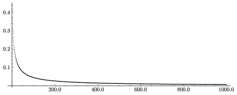
Figure 1. The topological entropy $\mathcal{H}_{m}$ for $1\leqslant m\leqslant 1000$.

The set of exact RNMS words facilitates a convenient method for the computation of the topological entropy. Applying a theorem of Nilsson [15, Thm. 3] and carrying out a short calculation, concerning the cardinalities of exact RNMS sets, yields the following result [11, Sec. 3.2] for the topological entropy $\mathcal{H}_{m}$ in the RNMS case.

$$\mathcal{H}_{m} =\lim_{k\to\infty}\frac{\log\bigl{(}\lvert\mathcal{G}_{m,k}\rvert\bigr{)}}{\ell_{m,k}}=\frac{\lambda_{m}-1}{1-\lambda_{m}^{\prime}}\sum_{i=2}^{\infty}\frac{\log\bigl{(}m(i-1)+1\bigr{)}}{\lambda_{m}^{i}},$$

which is strictly positive. This is in contrast to the deterministic cases of $\mathcal{N}_{m}$ where each element of $\mathbb{X}_{m,i}$ is a Sturmian sequence [11, Prop. 3.2] which means that the topological entropy vanishes here.

4. Ergodicity

In this section, we define a shift-invariant probability measure on the discrete RNMS hull $\mathbb{X}_{m}$ and prove its ergodicity. The result is somewhat weaker as in all deterministic cases of $\mathcal{N}_{m}$, because it is known that the hulls of primitive substitutions are minimal and that there is a uniquely ergodic probability measure [19]. As $\mathbb{X}_{m,i}\subsetneq\mathbb{X}_{m}$ [11, Prop. 2.22], one directly observes the non-minimality of $\mathbb{X}_{m}$ and the non-uniqueness of the measure can be expected immediately and will be proved explicitly later.

Definition 4.1.

Let $\ell\in\mathbb{N}$ and $\zeta_{m}\colon\mathcal{A}_{2}^{\ast}\longrightarrow\mathcal{A}_{2}^{\ast}$ be a random noble means substitution for some fixed $m\in\mathbb{N}$. Then, we refer to

$$(\zeta_{m})_{\ell}\colon\mathcal{D}_{m,\ell}^{\ast}\longrightarrow\mathcal{D}_{m,\ell}^{\ast}$$

as the induced substitution defined by

$$(\zeta_{m})_{\ell}\colon w^{(i)}\longmapsto\left\{\begin{array}[]{cc}u^{(i,1)}\mathrel{\mathop{:}\!\!=}\Bigl{(}v^{(i,1)}_{[k,k+\ell-1]}\Bigr{)}_{0\leqslant k\leqslant\lvert\zeta_{m}(w_{0}^{(i)})\rvert-1},&\text{with prob. }p_{i1},\\ \vdots&\vdots\\ u^{(i,n_{i})}\mathrel{\mathop{:}\!\!=}\Bigl{(}v^{(i,n_{i})}_{[k,k+\ell-1]}\Bigr{)}_{0\leqslant k\leqslant\lvert\zeta_{m}(w_{0}^{(i)})\rvert-1},&\text{with prob. }p_{in_{i}},\\ \end{array}\right.$$

where $w^{(i)}\in\mathcal{D}_{m,\ell}$ and $v^{(i,j)}\in\mathcal{D}_{m}$ is an image of $w^{(i)}$ under $\zeta_{m}$ with probability $p_{ij}$.

One can show that the induced substitution matrix $M_{m,\ell}$ of $(\zeta_{m})_{\ell}$ is primitive [11, Prop. 4.7] which enables the reapplication of Perron–Frobenius theory. Note that $(\zeta_{m})_{1}=\zeta_{m}$ and therefore $M_{m,1}=M_{m}$. In the case of $\ell=2$, one can explicitly work out $M_{m,2}$ for arbitrary $m\in\mathbb{N}$ [11, Prop. 4.10] and proceed recursively for the generalisation to any word length $\ell\in\mathbb{N}$ [11, Cor. 4.13]. One finds

$$M_{m,2}=\begin{pmatrix}m-1+p_{0}p_{m}&m-1+p_{0}&1-p_{0}&1\\ 1-p_{0}p_{m}&1-p_{0}&p_{0}&0\\ 1-p_{0}p_{m}&1&0&0\\ p_{0}p_{m}&0&0&0\end{pmatrix},$$

with statistically normalised right PF eigenvector

$$\bm{R}_{m,2}=\begin{pmatrix}\frac{2(\lambda_{m}-1)}{m(1+p_{0}p_{m})-(2+2\lambda_{m}-m)(-1+p_{0}p_{m})}\\ \frac{2(1-p_{0}p_{m})}{m(1+p_{0}p_{m})-(2+2\lambda_{m}-m)(-1+p_{0}p_{m})}\\ \frac{2(1-p_{0}p_{m})}{m(1+p_{0}p_{m})-(2+2\lambda_{m}-m)(-1+p_{0}p_{m})}\\ \frac{2(1+\lambda_{m}^{\prime})p_{0}p_{m}}{m(1+p_{0}p_{m})-(2+2\lambda_{m}-m)(-1+p_{0}p_{m})}\end{pmatrix}.$$ (3)

Now, let $w\in\mathcal{D}_{m,\ell}$ be any $\zeta_{m}$-legal word. Then, we define the measure $\mu_{m}$ on the cylinder sets $\mathcal{Z}_{k}(w)$ by

$$\mu_{m}\bigl{(}\mathcal{Z}_{k}(w)\bigr{)}\mathrel{\mathop{:}\!\!=}\bm{R}_{m,\ell}(w),$$ (4)

for any $k\in\mathbb{Z}$, where $\bm{R}_{m,\ell}(w)$ is the entry of the statistically normalised right PF eigenvector of $M_{m,\ell}$ with respect to the word $w$. According to [19, Sec. 5.4], this is a consistent definition of a measure on $\mathfrak{Z}(\mathbb{X}_{m})$ and there is an extension of $\mu_{m}$ to the Borel $\sigma$-algebra $\mathfrak{B}_{m}$ [17, Cor. 2.4.9] generated by the cylinder sets. Due to [17, Prop. 2.5.1], this extension is unique and we will denote it again as $\mu_{m}$. Note that Eq. $\eqref{equ:induced_right_pf}$ indicates that $\mu_{m}$ depends on the choice of $\bm{p}_{m}$, whereas the hull $\mathbb{X}_{m}$ is invariant under alterations of the choosing probabilities as long as $\bm{p}_{m}\gg 0$. The same is true for any $\ell\in\mathbb{N}$ which means that there are infinitely many possibilities to construct a probability measure for the very same $\mathbb{X}_{m}$ in the above way. We proceed with an important ingredient for the proof of the ergodicity of $\mu_{m}$.

Theorem 4.2 ([4, Thm. 1]).

Let $(X_{i})_{i\in\mathbb{N}}$ be a family of pairwise independent, identically distributed, complex random variables with common distribution $\mu$, subject to the integrability condition $\mathbb{E}_{\mu}(\lvert X_{1}\rvert)<\infty$. Then,

$$\frac{1}{n}\sum_{i=1}^{n}X_{i}\;\xrightarrow[\text{a.s.}]{n\to\infty}\;\mathbb{E}_{\mu}(X_{1})=\int_{\mathbb{R}}x\mathop{}\!\mathrm{d}\mu(x).$$ ∎

Here, $\mathbb{E}_{\mu}(X)$ denotes the mean of the random variable $X$ with respect to the distribution $\mu$.

Proposition 4.3.

For an arbitrary but fixed $m\in\mathbb{N}$, let $\mathbb{X}_{m}\subset\mathcal{A}_{2}^{\mathbb{Z}}$ be the two-sided discrete stochastic hull of the random noble means substitution and $\mu_{m}$ be the $S$-invariant probability measure on $\mathbb{X}_{m}$ introduced in Eq. $\eqref{equ:ergodic_meas}$. For any $f\in L^{1}(\mathbb{X}_{m},\mu_{m})$ and for an arbitrary but fixed $s\in\mathbb{Z}$, the identity

$$\lim_{n\to\infty}\frac{1}{n}\sum_{i=s}^{n+s-1}f(S^{i}x)=\int_{\mathbb{X}_{m}}f\mathop{}\!\mathrm{d}\mu_{m}$$ (5)

holds for $\mu_{m}$-almost every $x\in\mathbb{X}_{m}$.

• Let $x\in\mathbb{X}_{m}$ be an arbitrary element of the stochastic hull. The idea is to consider the characteristic function $\mathbbm{1}_{\mathcal{Z}}$ of some cylinder set $\mathcal{Z}\in\mathfrak{Z}(\mathbb{X}_{m})$ and to interpret $X\mathrel{\mathop{:}\!\!=}\bigl{(}\mathbbm{1}_{\mathcal{Z}}(S^{i}x)\bigr{)}_{i\in\mathbb{N}}$ as a family of $\mu_{m}$-distributed random variables in order to invoke Theorem 4.2. For this purpose, we have to deal with the pairwise independence of elements in $X$. One can show that there is at least one element $x^{\prime}\in\mathbb{X}_{m}$ with $\zeta_{m}(x^{\prime})\operatorname{\,\leavevmode\hbox{\set@color\hskip 7.7778pt\leavevmode\hbox{\set@color=}\raisebox{7.16875pt}{\rule{2.5pt}{0.0pt}{\tiny\scalebox{0.75}{$\bullet$}}\rule{2.5pt}{0.0pt}}}\,}x$ [11, Rem. 2.25] which means that we can study the structure of $x$ that is induced by the action of $\zeta_{m}$ on some element of $\mathbb{X}_{m}$. For two finite subwords $u$, $v\in\mathcal{D}_{m,\ell}$ of $x$, we denote by $u\Cap v$ the overlap of $u$ and $v$ in $x$ and by $\lvert u\Cap v\rvert$ its number of letters. Certainly, $u$ and $v$ cannot be independent if $\lvert u\Cap v\rvert>0$, but we have to take more into account. Possibly, $u$ and $v$ may contain parts of the image of the same letter under $\zeta_{m}$. As $\lvert\zeta_{m}(\mathtt{a})\rvert=m+1>1=\lvert\zeta_{m}(\mathtt{b})\rvert$, it is sufficient to ensure that at most one of the overlaps $u\Cap\zeta_{m}(\mathtt{a})$ and $v\Cap\zeta_{m}(\mathtt{a})$ is non-empty for the very same letter $\mathtt{a}\vartriangleleft x^{\prime}$, as illustrated in Figure 2.

  Figure 2. The words $u$, $v\in\mathcal{D}_{m,\ell}$ are independent as of the shift by $\ell+m$ positions. The word $\zeta_{m}(\mathtt{a})$ can have non-empty overlap with precisely one of the two words.

  Now, define for any $i\in\mathbb{Z}$, $\ell\in\mathbb{N}$ and a fixed $t\in\mathbb{Z}$, the family

  $$(X_{i,k})_{k\in\mathbb{N}_{0}}\mathrel{\mathop{:}\!\!=}\Bigl{(}\bigl{(}S^{i+k(\ell+m)}x\bigr{)}_{[t,t+\ell-1]}\Bigr{)}_{k\in\mathbb{N}_{0}}.$$

  Then, each $X\in\bigl{\{}(X_{i,k})_{k\in\mathbb{N}_{0}}\mid s\leqslant i\leqslant\ell+m+s-1\bigr{\}}$ consists of pairwise independent words in the sense pointed out above. Furthermore, for any $v\in\mathcal{D}_{m,\ell}$, we consider the characteristic function of the cylinder set $\mathcal{Z}_{t}(v)\leavevmode\nobreak\ \in\leavevmode\nobreak\ \mathfrak{Z}(\mathbb{X}_{m})$, defined by

  $$\mathbbm{1}_{\mathcal{Z}_{t}(v)}(x)\mathrel{\mathop{:}\!\!=}\left\{\begin{array}[]{ll}1,&\text{if }x_{[t,t+\ell-1]}=v,\\ 0,&\text{otherwise.}\end{array}\right.$$

  This leads to

  $$\lim_{n\to\infty}\frac{1}{n} \sum_{i=s}^{n+s-1}\mathbbm{1}_{\mathcal{Z}_{t}(v)}(S^{i}x)$$

  $$=\lim_{n\to\infty}\frac{1}{n}\sum_{i=s}^{\ell+m+s-1}\sum_{k=0}^{\lfloor\frac{n-1-i}{\ell+m}\rfloor}\mathbbm{1}_{\mathcal{Z}_{t}(v)}\bigl{(}S^{i+k(\ell+m)}x\bigr{)}$$

  $$=\lim_{n\to\infty}\frac{1}{\ell+m}\sum_{i=s}^{\ell+m+s-1}\frac{1}{\lfloor\frac{n-1-i}{\ell+m}\rfloor+1}\sum_{k=0}^{\lfloor\frac{n-1-i}{\ell+m}\rfloor}\mathbbm{1}_{\mathcal{Z}_{t}(v)}\bigl{(}S^{i+k(\ell+m)}x\bigr{)}.$$ (6)

  For $$s\leqslant i\leqslant\ell+m+s-1 \bigl{(}\mathbbm{1}_{\mathcal{Z}_{t}(v)}(S^{i+k(\ell+m)}x)\bigr{)}_{k\in\mathbb{N}_{0}} \eqref{equ:slln_apply} \eqref{equ:slln_apply}$$, we consider the family and apply Theorem 4.2 to each of the inner sums of Eq.  separately and appropriately put the resulting means together. Thus, Eq.  is almost surely

  $$=\frac{1}{\ell+m}\sum_{i=s}^{\ell+m+s-1}\mathbb{E}_{\mu_{m}}\bigl{(}\mathbbm{1}_{\mathcal{Z}_{t}(v)}(S^{i}x)\bigr{)}=\mathbb{E}_{\mu_{m}}\bigl{(}\mathbbm{1}_{\mathcal{Z}_{t}(v)}(x)\bigr{)}$$

  $$=\int_{\mathbb{X}_{m}}\mathbbm{1}_{\mathcal{Z}_{t}(v)}\mathop{}\!\mathrm{d}\mu_{m}.$$

  Note that the penultimate equality is implied by the Perron–Frobenius Theorem and the uniqueness of $\bm{R}_{m,\ell}$ stated therein.

  To finish the proof, we need to extend the presented arguments to an arbitrary function in $L^{1}(\mathbb{X}_{m},\mu_{m})$. We define

  $$\Gamma\mathrel{\mathop{:}\!\!=}\Bigl{\{}\sum_{\mathcal{Z}\in S}a_{\mathcal{Z}}\mathbbm{1}_{\mathcal{Z}}\mid S\subset\mathfrak{Z}(\mathbb{X}_{m})\text{ finite and }a_{\mathcal{Z}}\in\mathbb{C}\Bigr{\}}$$

  as the set of simple functions on the measure space $\bigl{(}\mathbb{X}_{m},\mathfrak{B}_{m},\mu_{m}\bigr{)}$. By linearity, the validity of Eq. $\eqref{equ:ergodic}$ for $\mathbbm{1}_{\mathcal{Z}_{t}(v)}$ extends to an arbitrary function in $\Gamma$. Due to the Stone–Weierstraß theorem [8, Thm. 1.4], $\Gamma$ is dense in $\mathcal{C}(\mathbb{X}_{m})$ and thus also in $L^{1}(\mathbb{X}_{m},\mu_{m})$ [8, Thm. 3.1]. This implies the assertion. ∎

  Theorem 4.4.

  The measure $\mu_{m}$ is ergodic.

• This is an immediate consequence of Proposition 4.3. via an application of Birkhoff’s ergodic theorem. ∎

5. Cut and project

The geometric realisation of fixed points of elements in $\mathcal{N}_{m}$ is derived from the left PF eigenvector $(\lambda_{m},1)^{T}$ of $M_{m}$ via the identification of $\mathtt{a}$ and $\mathtt{b}$ with intervals of lengths $\lambda_{m}$ and $1$ and using the left endpoints as coordinates. Each of these realisations is called a noble means set and is denoted by $\Lambda_{m,i}$. It can be shown [11, Cor. 5.17 and Cor. 5.18] that all $\Lambda_{m,i}$ can be identified as so-called model sets $\Theta(W_{m,i})$ with windows $W_{m,i}$ within the cut and project scheme $\mathfrak{C}\mathrel{\mathop{:}\!\!=}(\mathbb{R},\mathbb{R},\mathcal{L}_{m})$; see Figure 3 for a compact representation and we refer to [1, Cha. 7] for a general introduction. The underlying lattice $\mathcal{L}_{m}\mathrel{\mathop{:}\!\!=}\{(x,x^{\prime})\mid x\in\mathbb{Z}[\lambda_{m}]\}$ is independent of $i$. Note that, for the generic cases $0<i<m$, we find the windows

$$W_{m,i}=i\tau_{m}+[\lambda_{m}^{\prime},1]\quad\text{with}\quad\tau_{m}\mathrel{\mathop{:}\!\!=}-\frac{1}{m}(\lambda_{m}^{\prime}+1).$$ (7)

In the singular cases $i\in\{0,m\}$, we get

$$W_{m,0}^{(\mathtt{a}|\mathtt{a})} \mathrel{\mathop{:}\!\!=}[\lambda_{m}^{\prime},1), W_{m,0}^{(\mathtt{a}|\mathtt{b})} \mathrel{\mathop{:}\!\!=}(\lambda_{m}^{\prime},1],$$ (8)

$$\quad W_{m,m\vphantom{0}}^{(\mathtt{a}|\mathtt{a})} \mathrel{\mathop{:}\!\!=}(-1,-\lambda_{m}^{\prime}], \quad W_{m,m\vphantom{0}}^{(\mathtt{b}|\mathtt{a})} \mathrel{\mathop{:}\!\!=}[-1,-\lambda_{m}^{\prime}),$$ (9)

distinguished according to the legal two-letter seeds. In the randomised situation, we consider the geometric realisation of generating random noble means words and study the same cut and project scheme $\mathfrak{C}$ as in the deterministic cases. In this context, we find the following result.

Figure 3. Cut and project scheme for the noble means sets $\Lambda_{m,i}$.

Proposition 5.1.

Let $\Lambda_{m}$ be a generating random noble means set. Then, $\Lambda_{m}\subset\Theta\bigl{(}W_{m}\bigr{)}$ with $W_{m}\mathrel{\mathop{:}\!\!=}[\lambda_{m}^{\prime}-1,1-\lambda_{m}^{\prime}]$.

• Assume there is a set $W_{m}=A\cup B$ in the internal space with the property $\Lambda_{m}\subset\Theta(W_{m})=\Theta(A)\cup\Theta(B)$. Here, the sets $\Theta(A)$ and $\Theta(B)$ denote the left endpoints of intervals generated by the letters $\mathtt{a}$ and $\mathtt{b}$, respectively. If $\Lambda_{m}$ is a generating random noble means set, the same is true for $\zeta_{m}(\Lambda_{m})$, and the sought-after sets $\Theta(A)$ and $\Theta(B)$ are invariant under $\zeta_{m}$. Now, consider $x\in\Lambda_{m}$ and note that the interval $[0,x]$ is always mapped to the interval $\lambda_{m}\cdot[0,x]$. The sets $\Theta(A)$ and $\Theta(B)$ are consequently invariant under $\zeta_{m}$ if and only if for all $0\leqslant i\leqslant m$ the inclusions

  $$\zeta_{m,i}\bigl{(}\Theta(A)\bigr{)}\subset\Theta(A)\quad\text{and}\quad\zeta_{m,i}\bigl{(}\Theta(B)\bigr{)}\subset\Theta(B)$$

  hold. As conditions in the physical space, we get for $0\leqslant i\leqslant m$ the $m+1$ systems

  $$\Theta(A) \supset\biggl{\{}\bigcup_{j=0}^{i-1}\lambda_{m}\Theta(A)+j\lambda_{m}\biggr{\}}\cup\lambda_{m}\Theta(B)\cup\biggl{\{}\bigcup_{j=i}^{m-1}\lambda_{m}\Theta(A)+j\lambda_{m}+1\biggr{\}}$$

  $$\Theta(B) \supset\lambda_{m}\Theta(A)+i\lambda_{m}$$

  and in the internal space the corresponding conjugate systems

  $$A \supset\biggl{\{}\bigcup_{j=0}^{i-1}\lambda^{\prime}_{m}A+j\lambda^{\prime}_{m}\biggr{\}}\cup\lambda_{m}^{\prime}B\cup\biggl{\{}\bigcup_{j=i}^{m-1}\lambda^{\prime}_{m}A+j\lambda^{\prime}_{m}+1\biggr{\}}$$ (10)

  $$B \supset\lambda^{\prime}_{m}A+i\lambda^{\prime}_{m}.$$

  As only affine maps appear in Eq. $\eqref{equ:superwindow_conditions}$, it suffices to investigate the extremal cases $i=0$ and $i=m$. Furthermore, we can assume that $A$ and $B$ are closed intervals, because if $C\in\{A,B\}$ satisfies all conditions of Eq. $\eqref{equ:superwindow_conditions}$ and is no interval, then define $\overline{C}=[\inf C,\sup C]$. As all involved maps are affine, $\overline{C}$ also meets these conditions and we may define $A\mathrel{\mathop{:}\!\!=}[\alpha,\beta]$ and $B\mathrel{\mathop{:}\!\!=}[\gamma,\delta]$. Among the remaining conditions of Eq. $\eqref{equ:superwindow_conditions}$, only the following six are not redundant:

  $$\begin{array}[]{lll}(1)\;\lambda_{m}^{\prime}\bigl{(}\beta+(m-1)\bigr{)}\geqslant\alpha&\;(2)\;\lambda_{m}^{\prime}\delta\geqslant\alpha&\;(3)\;\lambda_{m}^{\prime}\gamma\leqslant\beta\\ (4)\;\lambda_{m}^{\prime}(\beta+m)\geqslant\gamma&\;(5)\;\lambda_{m}^{\prime}\alpha+1\leqslant\beta&\;(6)\;\lambda_{m}^{\prime}\alpha\leqslant\delta.\end{array}$$

  Because of Eqs. $\eqref{equ:window_1}$ to $\eqref{equ:window_3}$, we may assert the relative position $\gamma<\alpha\leqslant\delta<\beta$ of $A$ to $B$. This appears to be a linear optimisation problem, which is not uniquely solvable in general. Consequently, we additionally demand that the interval $W_{m}=[\gamma,\beta]$ be minimal, which leads to the condition $\lambda_{m}^{\prime}(\beta+m)=\gamma$. This equation describes the largest translation to the left and if $\lambda_{m}^{\prime}(\beta+m)>\gamma$, the length of $W_{m}$ was not minimal. By solving the linear optimisation problem of Eq. $\eqref{equ:superwindow_conditions}$ under consideration of all given boundary conditions, we get the intervals

  $$A=[-1,1-\lambda_{m}^{\prime}],\quad B=[\lambda_{m}^{\prime}-1,-\lambda_{m}^{\prime}]\quad\text{and}\quad W_{m}=[\lambda_{m}^{\prime}-1,1-\lambda_{m}^{\prime}].$$

  These intervals actually satisfy Eq. $\eqref{equ:superwindow_conditions}$, because for $i=m$ we get

  $$\biggl{\{}\bigcup_{j=0}^{m-1}\lambda_{m}^{\prime}A+j\lambda_{m}^{\prime}\biggr{\}}\cup\lambda_{m}^{\prime}B =[-(\lambda_{m}^{\prime})^{2}+m\lambda_{m}^{\prime},-\lambda_{m}^{\prime}]$$

  $$\qquad\cup[-1-m\lambda_{m}^{\prime},1+(m-1)\lambda_{m}^{\prime}]$$

  $$=[-1,-\lambda_{m}^{\prime}]\cup[-1-m\lambda_{m}^{\prime},1+(m-1)\lambda_{m}^{\prime}]$$

  $$\subset[-1,1-\lambda_{m}^{\prime}]=A$$

  and

  $$\lambda_{m}^{\prime}A+m\lambda_{m}^{\prime} =[-(\lambda_{m}^{\prime})^{2}+(m+1)\lambda_{m}^{\prime},(m-1)\lambda_{m}^{\prime}]$$

  $$=[\lambda_{m}^{\prime}-1,(m-1)\lambda_{m}^{\prime}]$$

  $$\subset[\lambda_{m}^{\prime}-1,-\lambda_{m}^{\prime}]=B.$$

  Analogously, we get the corresponding inclusions for $i=0$. Furthermore, the minimality condition of $W_{m}$ is fulfilled because

  $$\lambda_{m}^{\prime}(\beta+m)=\lambda_{m}^{\prime}(1-\lambda_{m}^{\prime}+m)=\lambda_{m}^{\prime}-1=\gamma.\qed$$

  Henceforth, we indicate the continuous random noble means hull by $\mathbb{Y}_{m}$ and denote any element in $\mathbb{Y}_{m}$ as a random noble means set. We refer to [11, Cha. 5] for a broader overview in this regard.

  Theorem 5.2.

  Each random noble means set $\Lambda\in\mathbb{Y}_{m}$ is Meyer.

• Let $\Lambda_{m}$ be a generating random noble means set. Evidently, $\Lambda_{m}$ is relatively dense in $\mathbb{R}$ with covering radius $\lambda_{m}/2$ and, by Proposition 5.1, it is a subset of the model set $\Theta\bigl{(}[\lambda_{m}^{\prime}-1,1-\lambda_{m}^{\prime}]\bigr{)}$. The Meyer property of $\Lambda_{m}$ then follows from [14, Thm. 9.1]. We know that there is a generating random noble means set whose orbit is dense, $\Lambda_{m}$ say. Now, choose an arbitrary random noble means set $\Lambda\in\mathbb{Y}_{m}$ and a converging sequence $(t_{n}+\Lambda_{m})_{n\in\mathbb{N}}$ with limit $\Lambda$. For any $n\in\mathbb{N}$, we find

  $$(t_{n}+\Lambda_{m})-(t_{n}+\Lambda_{m})=\Lambda_{m}-\Lambda_{m}$$

  and therefore $\Lambda-\Lambda\subset\Lambda_{m}-\Lambda_{m}$ which means that $\Lambda$ is uniformly discrete. As the relative denseness of $\Lambda$ is clear, this proves the assertion. ∎

6. Diffraction measure

In this last section, we present some results concerning the spectral nature of the diffraction measure of typical random noble means sets. We refer to [1, Chs. 8 and 9] for a detailed and readable introduction to diffraction theory of model sets; compare [1].

To begin with, we briefly discuss the deterministic cases of $\mathcal{N}_{m}$ that can be treated with results from the general theory.

Lemma 6.1.

For an arbitrary but fixed $m\in\mathbb{N}$ and $0\leqslant i\leqslant m$, the diffraction measure of $\Lambda_{m,i}$ is a positive and positive definite, translation bounded, pure point measure. It is explicitly given by

$$\widehat{\gamma_{\Lambda_{m,i}}}=\sum_{k\in\mathcal{L}_{m}^{\circledast}}\lvert A_{m,i}(k)\rvert^{2}\,\delta_{k},$$ (11)

with the amplitudes

$$A_{m,i}(k)=\operatorname{dens}(\Lambda_{m,i})\operatorname{e}^{-\pi\hskip 0.5pt\mathrm{i}\hskip 0.5ptk^{\star}(\lambda_{m}^{\prime}+1)(1-2i/m)}\operatorname{sinc}\bigl{(}\pi k^{\star}(1-\lambda_{m}^{\prime})\bigr{)}.$$

• To begin with, we note that the Fourier transform of the characteristic function of an interval $[a,b]\subset\mathbb{R}$ can be represented as

  $$\widehat{\mathbbm{1}_{[a,b]}}(x)=(b-a)\operatorname{e}^{-\pi\hskip 0.5pt\mathrm{i}\hskip 0.5ptx(a+b)}\operatorname{sinc}\bigl{(}\pi x(b-a)\bigr{)},$$ (12)

  where $\operatorname{sinc}(z)\mathrel{\mathop{:}\!\!=}\sin(z)/z$. A short calculation based on [20, Thm. 1] yields $\operatorname{dens}(\Lambda_{m,i})=(1-\lambda_{m}^{\prime})/\sqrt{m^{2}+4}$. Combining this with [1, Thm. 9.4] and Eqs. $\eqref{equ:window_1}$ to $\eqref{equ:window_3}$, we find

  $$A_{m,i}(k) =\frac{\operatorname{dens}(\Lambda_{m,i})}{\operatorname{vol}(W_{m,i})}\widehat{\mathbbm{1}_{W_{m,i}}}(-k^{\star})$$

  $$=\frac{(1-\lambda_{m}^{\prime})\operatorname{e}^{-\pi\hskip 0.5pt\mathrm{i}\hskip 0.5ptk^{\star}(\lambda_{m}^{\prime}+1)(1-2i/m)}\operatorname{sinc}\bigl{(}\pi k^{\star}(1-\lambda_{m}^{\prime})\bigr{)}}{\sqrt{m^{2}+4}}$$

  $$=\operatorname{dens}(\Lambda_{m,i})\operatorname{e}^{-\pi\hskip 0.5pt\mathrm{i}\hskip 0.5ptk^{\star}(\lambda_{m}^{\prime}+1)(1-2i/m)}\operatorname{sinc}\bigl{(}\pi k^{\star}(1-\lambda_{m}^{\prime})\bigr{)},$$

  by an application of Eq. $\eqref{equ:transform_char_func}$. ∎ In the stochastic situation, we first have to take a closer look at the autocorrelation $\gamma_{\Lambda,m}$ of any $\Lambda\in\mathbb{Y}_{m}$, which is defined by

  $$\gamma_{\Lambda,m}\mathrel{\mathop{:}\!\!=}\delta_{\Lambda}\circledast\widetilde{\delta_{\Lambda}}\mathrel{\mathop{:}\!\!=}\lim_{n\to\infty}\frac{\delta_{\Lambda_{n}}\ast\widetilde{\delta_{\Lambda_{n}}}}{\operatorname{vol}(B_{n})}\quad\text{with}\quad\Lambda_{n}\mathrel{\mathop{:}\!\!=}B_{n}(0)\cap\Lambda.$$

  Via regularisation of $\delta_{\Lambda}$ and an application of the ergodic theorem for continuous functions [13, Thm. 2.14z], we find that

  $$\gamma_{\Lambda,m}=\mathbb{E}_{\nu_{m}}\bigl{(}\delta_{\Lambda}\circledast\widetilde{\delta_{\Lambda}}\bigr{)}$$

  with $\nu_{m}$ the measure induced by suspension ([3, Cha. 11] and [11, Sec. 6.1]) of $\mu_{m}$. Here, $\gamma_{\Lambda,m}$ is positive definite by construction and its Fourier transform exists due to [2, Sec. 4]. We find

  $$\widehat{\gamma_{\Lambda,m}} =\bigl{(}\mathbb{E}_{\nu_{m}}(\delta_{\Lambda}\circledast\widetilde{\delta_{\Lambda}})\bigr{)}^{\widehat{}}=\lim_{n\to\infty}\mathbb{E}_{\nu_{m}}\Bigl{(}\frac{1}{\operatorname{vol}(B_{n})}\widehat{\delta_{\Lambda_{n}}}\widehat{\widetilde{\delta_{\Lambda_{n}}}}\Bigr{)}$$

  $$=\lim_{n\to\infty}\frac{1}{\operatorname{vol}(B_{n})}\mathbb{E}_{\nu_{m}}\Bigl{(}\widehat{\delta_{\Lambda_{n}}}\overline{\widehat{\delta_{\Lambda_{n}}}}\Bigr{)}=\lim_{n\to\infty}\frac{1}{\operatorname{vol}(B_{n})}\mathbb{E}_{\nu_{m}}(\lvert X_{n}\rvert^{2})$$

  $$=\lim_{n\to\infty}\frac{1}{\operatorname{vol}(B_{n})}\lvert\mathbb{E}_{\nu_{m}}(X_{n})\rvert^{2}+\lim_{n\to\infty}\frac{1}{\operatorname{vol}(B_{n})}\bigl{(}\mathbb{E}_{\nu_{m}}(\lvert X_{n}\rvert^{2})-\lvert\mathbb{E}_{\nu_{m}}(X_{n})\rvert^{2}\bigr{)}$$

  $$=\lim_{n\to\infty}\frac{1}{\operatorname{vol}(B_{n})}\lvert\mathbb{E}_{\nu_{m}}(X_{n})\rvert^{2}+\lim_{n\to\infty}\frac{1}{\operatorname{vol}(B_{n})}\mathbb{V}_{\nu_{m}}(X_{n}),$$ (13)

  where $\mathbb{V}_{\nu_{m}}(X_{n})$ is the variance of

  $$X_{n}(k)\mathrel{\mathop{:}\!\!=}\sum_{x\in\Lambda_{n}}\operatorname{e}^{-2\pi\hskip 0.5pt\mathrm{i}\hskip 0.5ptkx}=\sum_{x\in\Lambda_{n}}\widehat{\delta_{x}},$$

  provided that all limits exist. The idea of breaking up $\widehat{\gamma_{\Lambda,m}}$ according to first and second moments will result in $\lim_{n\to\infty}\lvert\mathbb{E}_{\nu_{m}}(X_{n})\rvert^{2}/\operatorname{vol}(B_{n})$ containing the pure point part and $\lim_{n\to\infty}\mathbb{V}_{\nu_{m}}(X_{n})/\operatorname{vol}(B_{n})$ being the absolutely continuous part of $\widehat{\gamma_{\Lambda,m}}$. In the following, we will restrict to the special case of $m=1$ and consider suitable subsequences to ensure the convergence in Eq. $\eqref{equ:diffr_rek}$. The general case of $m\in\mathbb{N}$ can be treated similarly.

  For $n\geqslant 2$, we define the sequence

  $$L_{n}\mathrel{\mathop{:}\!\!=}L_{n-1}+L_{n-2}\quad\text{with}\quad L_{0}\mathrel{\mathop{:}\!\!=}1\quad\text{and}\quad L_{1}\mathrel{\mathop{:}\!\!=}\lambda_{1}$$

  that possesses the closed form $L_{n}=\lambda_{1}^{n}$ for any $n\in\mathbb{N}$ and furthermore, we set

  $$X_{n}(k)\mathrel{\mathop{:}\!\!=}\left\{\begin{array}[]{ll}X_{n-2}(k)+\operatorname{e}^{-2\pi\hskip 0.5pt\mathrm{i}\hskip 0.5ptkL_{n-2}}X_{n-1}(k),&\text{with probability }p_{0},\\ X_{n-1}(k)+\operatorname{e}^{-2\pi\hskip 0.5pt\mathrm{i}\hskip 0.5ptkL_{n-1}}X_{n-2}(k),&\text{with probability }p_{1},\end{array}\right.$$ (14)

  where $X_{0}(k)\mathrel{\mathop{:}\!\!=}\operatorname{e}^{-2\pi\hskip 0.5pt\mathrm{i}\hskip 0.5ptk}$ and $X_{1}(k)\mathrel{\mathop{:}\!\!=}\operatorname{e}^{-2\pi\hskip 0.5pt\mathrm{i}\hskip 0.5ptk\lambda_{1}}$. Moreover, we define the sequences

  $$\bigl{(}\mathcal{P}_{n}\bigr{)}_{n\in\mathbb{N}_{0}}\mathrel{\mathop{:}\!\!=}\Bigl{(}\frac{1}{L_{n}}\lvert\mathbb{E}(X_{n})\rvert^{2}\Bigr{)}_{n\in\mathbb{N}_{0}}\quad\text{and}\quad\bigl{(}\mathcal{S}_{n}\bigr{)}_{n\in\mathbb{N}_{0}}\mathrel{\mathop{:}\!\!=}\Bigl{(}\frac{1}{L_{n}}\mathbb{V}(X_{n})\Bigr{)}_{n\in\mathbb{N}_{0}},$$ (15)

  and derive results on the convergence of $(\mathcal{P}_{n})_{n\in\mathbb{N}_{0}}$ and $(\mathcal{S}_{n})_{n\in\mathbb{N}_{0}}$.

  We proceed with the derivation of recursion formulas for $\mathbb{E}\bigl{(}X_{n}(k)\bigr{)}$ and $\mathbb{V}\bigl{(}X_{n}(k)\bigr{)}$. For the sake of readability, we introduce the following abbreviations.

  $$\begin{gathered}\operatorname{e}_{n}\mathrel{\mathop{:}\!\!=}\operatorname{e}^{-2\pi\hskip 0.5pt\mathrm{i}\hskip 0.5ptkL_{n}},\quad\cos_{n}\mathrel{\mathop{:}\!\!=}\cos(2\pi kL_{n}),\quad X_{n}\mathrel{\mathop{:}\!\!=}X_{n}(k),\\ \mathbb{E}_{n}\mathrel{\mathop{:}\!\!=}\mathbb{E}\bigl{(}X_{n}(k)\bigr{)}\quad\text{and}\quad\mathbb{V}_{n}\mathrel{\mathop{:}\!\!=}\mathbb{E}\bigl{(}\bigl{\lvert}X_{n}(k)\bigr{\rvert}^{2}\bigr{)}-\bigl{\lvert}\mathbb{E}\bigl{(}X_{n}(k)\bigr{)}\bigr{\rvert}^{2},\end{gathered}$$ (16)

  for any $n\in\mathbb{N}$ and $k\in\mathbb{R}$. Using the definition of $X_{n}$ in Eq. $\eqref{equ:random_var}$, it is immediate that for $n\geqslant 2$, we have

  $$\mathbb{E}_{n} =\mathbb{E}\bigl{(}p_{0}(X_{n-2}+\operatorname{e}_{n-2}X_{n-1})+p_{1}(X_{n-1}+\operatorname{e}_{n-1}X_{n-2})\bigr{)}$$ (17)

  $$=(p_{1}+p_{0}\operatorname{e}_{n-2})\mathbb{E}_{n-1}+(p_{0}+p_{1}\operatorname{e}_{n-1})\mathbb{E}_{n-2},$$

  where $\mathbb{E}_{0}=\mathrm{e}^{-2\pi\mathrm{i}k}$ and $\mathbb{E}_{1}=\mathrm{e}^{-2\pi\mathrm{i}k\lambda_{1}}$. Firstly, we consider the sequence $(\mathcal{S}_{n})_{n\in\mathbb{N}_{0}}$. Applying Eq. $\eqref{equ:pp_rek}$ for any $n\geqslant 2$, we find

  $$\mathbb{V}_{n} =\mathbb{E}\bigl{(}p_{0}\lvert X_{n-2}+\operatorname{e}_{n-2}X_{n-1}\rvert^{2}+p_{1}\lvert X_{n-1}+\operatorname{e}_{n-1}X_{n-2}\rvert^{2}\bigr{)}-\lvert\mathbb{E}_{n}\rvert^{2}$$

  $$=\mathbb{V}_{n-1}+\mathbb{V}_{n-2}$$

  $$\qquad+2p_{0}p_{1}\Bigl{\{}\bigl{(}1-\cos_{n-2}\bigr{)}\lvert\mathbb{E}_{n-1}\rvert^{2}+\bigl{(}1-\cos_{n-1}\bigr{)}\lvert\mathbb{E}_{n-2}\rvert^{2}$$

  $$\qquad\qquad-\operatorname{Re}\bigl{[}\bigl{(}1-\overline{\operatorname{e}_{n-1}}-\operatorname{e}_{n-2}+\,\overline{\operatorname{e}_{n-1}}\operatorname{e}_{n-2}\bigr{)}\mathbb{E}_{n-1}\overline{\mathbb{E}_{n-2}}\bigr{]}\Bigr{\}}$$

  $$\qquad+2\operatorname{Re}\bigl{[}\bigl{(}p_{0}\operatorname{e}_{n-2}+p_{1}\overline{\operatorname{e}_{n-1}}\bigr{)}\bigl{(}\mathbb{E}(X_{n-1}\overline{X_{n-2}})-\mathbb{E}_{n-1}\overline{\mathbb{E}_{n-2}}\bigr{)}\bigr{]} \ast$$ ()

  $$=\mathbb{V}_{n-1}+\mathbb{V}_{n-2}+2p_{0}p_{1}\Psi_{n},$$

  with $\mathbb{V}_{0}=\mathbb{V}_{1}=0$ and

  $$\Psi_{n}\mathrel{\mathop{:}\!\!=}\Psi_{n}(k) \mathrel{\mathop{:}\!\!=}\bigl{(}1-\cos_{n-2}\bigr{)}\lvert\mathbb{E}_{n-1}\rvert^{2}+\bigl{(}1-\cos_{n-1}\bigr{)}\lvert\mathbb{E}_{n-2}\rvert^{2}$$

  $$\qquad-\operatorname{Re}\bigl{[}\bigl{(}1-\overline{\operatorname{e}_{n-1}}-\operatorname{e}_{n-2}+\overline{\operatorname{e}_{n-1}}\operatorname{e}_{n-2}\bigr{)}\mathbb{E}_{n-1}\overline{\mathbb{E}_{n-2}}\bigr{]}$$

  $$=\frac{1}{2}\bigl{\lvert}(1-\operatorname{e}_{n-2})\mathbb{E}_{n-1}-(1-\operatorname{e}_{n-1})\mathbb{E}_{n-2}\bigr{\rvert}^{2}\geqslant 0,$$ (18)

  for any $n\geqslant 2$. We have used that $\mathbb{E}(X_{n-1}\overline{X_{n-2}})-\mathbb{E}_{n-1}\overline{\mathbb{E}_{n-2}}=0$ in ($\ast$) which is a consequence of the independence of the random variables $X_{n}$ [11, Rem. 6.16]. Our study of the sequence $(\mathcal{S}_{n})_{n\in\mathbb{N}_{0}}$ proceeds with some preparing notes on the sequence $(\Psi_{n})_{n\geqslant 2}$; see also Figure 4.

  Lemma 6.2.

  For all $n\geqslant 2$, the function $\Psi_{n}$ is real analytic. Moreover, one has $\Psi_{n}(k)\leqslant 2$ and $\Psi_{n+1}(k)\leqslant\Psi_{n}(k)$ for all $k\in\mathbb{R}$.

• The representation of Eq. $\eqref{equ:delta_quad}$ immediately shows the analyticity of $\Psi_{n}$ because sums and products of trigonometric functions are real analytic. Next, we observe that

  $$\Psi_{2}(k) =\frac{1}{2}\big{\lvert}(1-\operatorname{e}^{-2\pi\hskip 0.5pt\mathrm{i}\hskip 0.5ptk})\operatorname{e}^{-2\pi\hskip 0.5pt\mathrm{i}\hskip 0.5ptk\lambda_{1}}-(1-\operatorname{e}^{-2\pi\hskip 0.5pt\mathrm{i}\hskip 0.5ptk\lambda_{1}})\operatorname{e}^{-2\pi\hskip 0.5pt\mathrm{i}\hskip 0.5ptk}\big{\rvert}^{2}$$

  $$=1-\cos\bigl{(}2\pi k(1-\lambda_{1})\bigr{)}\leqslant 2.$$

  Now, for $n\geqslant 2$ we define $\psi_{n}\mathrel{\mathop{:}\!\!=}\psi_{n}(k)\mathrel{\mathop{:}\!\!=}(1-\operatorname{e}_{n-2})\mathbb{E}_{n-1}-(1-\operatorname{e}_{n-1})\mathbb{E}_{n-2}$. Applying the recursion for $\mathbb{E}_{n}$ once on the first summand and using the recursion $L_{n}=L_{n-1}+L_{n-2}$ implies

  $$\psi_{n+1} =(1-\operatorname{e}_{n-1})\mathbb{E}_{n}-(1-\operatorname{e}_{n})\mathbb{E}_{n-1}=-(p_{0}+p_{1}\operatorname{e}_{n-1})\psi_{n}.$$ (19)

  This yields the monotonicity of $\Psi_{n}$ because

  $$\lvert\psi_{n+1}\rvert=\lvert p_{0}\psi_{n}+p_{1}\operatorname{e}_{n-1}\psi_{n}\rvert\leqslant p_{0}\lvert\psi_{n}\rvert+p_{1}\lvert\psi_{n}\rvert=\lvert\psi_{n}\rvert,$$

  and therefore

  $$\Psi_{n+1}(k)=\frac{1}{2}\lvert\psi_{n+1}(k)\rvert^{2}\leqslant\frac{1}{2}\lvert\psi_{n}(k)\rvert^{2}=\Psi_{n}(k).\qed$$

  

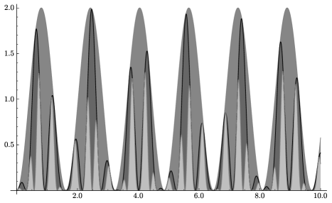
  Figure 4. The function $\Psi_{n}$ for $n=2$ (grey), $n=3$ (dark grey) and $n=4$ (light grey).

Proposition 6.3.

For any $n\in\mathbb{N}_{0}$, consider the function $\phi_{n}\colon\mathbb{R}\longrightarrow\mathbb{R}_{\geqslant 0}$, defined by

$$\phi_{n}(k)\mathrel{\mathop{:}\!\!=}\frac{1}{L_{n}}\mathbb{V}\bigl{(}X_{n}(k)\bigr{)}.$$

On $\mathbb{R}$, the sequence $(\phi_{n})_{n\in\mathbb{N}_{0}}$ converges uniformly to the continuous function $\phi\colon\mathbb{R}\longrightarrow\mathbb{R}_{\geqslant 0}$, with

$$\phi(k)\mathrel{\mathop{:}\!\!=}\frac{2p_{0}p_{1}\lambda_{1}}{\sqrt{5}}\sum_{i=2}^{\infty}\lambda_{1}^{-i}\Psi_{i}(k).$$ (20)

• From the recursion relation $\mathbb{V}_{n}=\mathbb{V}_{n-1}+\mathbb{V}_{n-2}+2p_{0}p_{1}\Psi_{n}$, we conclude the representation

  $$\lim_{n\to\infty}\phi_{n}(k)=\lim_{n\to\infty}\frac{2p_{0}p_{1}}{L_{n}}\sum_{i=2}^{n}\ell_{1,n+1-i}\Psi_{i}(k)=\frac{2p_{0}p_{1}\lambda_{1}}{\sqrt{5}}\sum_{i=2}^{\infty}\lambda_{1}^{-i}\Psi_{i}(k),$$

  where $\ell_{1,n}$ denotes the $n$th Fibonacci number as introduced after Eq. $\eqref{equ:concat_rule}$ on page 2. Next, we observe that $\phi$ is convergent because an application of Lemma 6.2 yields

  $$\phi(k)\leqslant\frac{4p_{0}p_{1}\lambda_{1}}{\sqrt{5}}\sum_{i=0}^{\infty}\lambda_{1}^{-i-2}=\frac{4p_{0}p_{1}\lambda_{1}}{\sqrt{5}}\leqslant\frac{\lambda_{1}}{\sqrt{5}}.$$

  Thus, $\phi$ is bounded and the sum consists of non-negative elements only. The uniformity of the convergence is implied by the following short calculation

  $$\lvert\phi_{n}(k)-\phi(k)\rvert =2p_{0}p_{1}\Bigl{\lvert}\sum_{i=2}^{n}\Bigl{(}\frac{\ell_{1,n+1-i}}{L_{n}}-\frac{\lambda_{1}^{1-i}}{\sqrt{5}}\Bigr{)}\Psi_{i}(k)-\sum_{i=n+1}^{\infty}\frac{\lambda_{1}^{1-i}}{\sqrt{5}}\Psi_{i}(k)\Bigr{\rvert}$$

  $$\leqslant 4p_{0}p_{1}\Bigl{(}\Bigl{\lvert}\frac{(\lambda_{1}^{\prime})^{n-1}}{\lambda_{1}^{n}\sqrt{5}}\sum_{i=0}^{n}(\lambda_{1}^{\prime})^{-i}\Bigr{\rvert}+\frac{1}{\lambda_{1}^{n}\sqrt{5}}\sum_{i=0}^{\infty}\lambda_{1}^{-i}\Bigr{)}$$

  $$\leqslant\Bigl{\lvert}\frac{(\lambda_{1}^{\prime})^{n-1}-1/(\lambda_{1}^{\prime})^{2}}{\lambda_{1}^{n}\sqrt{5}(1-1/\lambda_{1}^{\prime})}\Bigr{\rvert}+\frac{1}{\lambda_{1}^{n-2}\sqrt{5}},$$ (21)

  and both summands in the last line converge to zero, as $n\to\infty$. This means that

  $$\lim_{n\to\infty}\sup_{k\in\mathbb{R}}\,\lvert\phi_{n}(k)-\phi(k)\rvert=0,$$

  which at the same time implies the continuity of $\phi$. ∎

  Corollary 6.4.

  The roots of $\phi$ are precisely the roots of $\Psi_{2}$, and they are given by all integer multiples of $\lambda_{1}$.

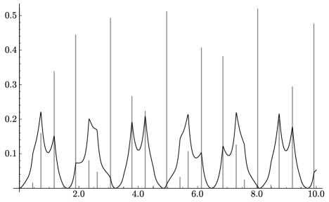
Figure 5. The pure point part (grey) and the absolutely continuous part (black) are illustrated for the case $m=1$ with $\bm{p}_{1}=(1/2,1/2)$.

• For $n\geqslant 1$, the recursion formula for $\psi_{n}$ in Eq. $\eqref{equ:rek_delta}$ can be rewritten as

  $$\psi_{n+1}(k) =(-1)^{n-1}\psi_{2}(k)\prod_{j=1}^{n-1}\bigl{(}p_{0}+p_{1}\operatorname{e}^{-2\pi\hskip 0.5pt\mathrm{i}\hskip 0.5ptkL_{j}}\bigr{)}$$

  $$=(-1)^{n-1}\bigl{(}\operatorname{e}^{-2\pi\hskip 0.5pt\mathrm{i}\hskip 0.5ptk\lambda_{1}}-\operatorname{e}^{-2\pi\hskip 0.5pt\mathrm{i}\hskip 0.5ptk}\bigr{)}\prod_{j=1}^{n-1}\bigl{(}p_{0}+p_{1}\operatorname{e}^{-2\pi\hskip 0.5pt\mathrm{i}\hskip 0.5ptkL_{j}}\bigr{)}.$$ (22)

  Considering each factor of the product in Eq. $\eqref{equ:rec_prod}$ separately and including $\Psi_{j}(k)=\lvert\psi_{j}(k)\rvert^{2}/2$ for any $j\geqslant 2$, we explore the function $f_{j}\colon\mathbb{R}\longrightarrow\mathbb{R}_{\geqslant 0}$ that is defined as

  $$f_{j}(k)\mathrel{\mathop{:}\!\!=}\bigl{\lvert}p_{0}+p_{1}\operatorname{e}^{-2\pi\hskip 0.5pt\mathrm{i}\hskip 0.5ptkL_{j}}\bigr{\rvert}^{2}=p_{0}^{2}+p_{1}^{2}+2p_{0}p_{1}\cos(2\pi kL_{j}).$$

  Here, for all $j\in\mathbb{N}$, the set of roots of $f_{j}$ reads

  $$R_{j}=\biggl{\{}\frac{\pm\arccos\bigl{(}\frac{2p_{0}p_{1}-1}{2p_{0}p_{1}}\bigr{)}+2\pi q}{2\pi L_{j}}\,\bigg{|}\,q\in\mathbb{Z}\biggr{\}}.$$

  Moreover, the expression $\lvert\operatorname{e}^{-2\pi\hskip 0.5pt\mathrm{i}\hskip 0.5ptk\lambda_{1}}-\operatorname{e}^{-2\pi\hskip 0.5pt\mathrm{i}\hskip 0.5ptk}\rvert^{2}=2-2\cos\bigl{(}2\pi k(1-\lambda_{1})\bigr{)}$ vanishes on all $k\in\lambda_{1}\mathbb{Z}$. This implies that

  $$\lambda_{1}\mathbb{Z}\cup\bigcup_{j=1}^{n-1}R_{j}$$

  is the set of roots of $\Psi_{n+1}$ for all $n\geqslant 1$. Because of Lemma 6.2 and the representation of $\phi$ in Eq. $\eqref{equ:radon_niko_density}$, this implies that $\lambda_{1}\mathbb{Z}$ is the set of roots of $\phi$. ∎

  

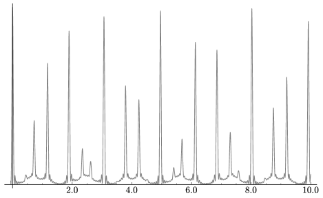
  Figure 6. Approximation of the diffraction measure for the case $m=1$ with $\bm{p}_{1}=(1/2,1/2)$, based on the recursion of Eq. $\eqref{equ:random_var}$ with $n=6$.

Finally, Proposition 6.3 implies the vague convergence of the sequence $(\mathcal{S}_{n})_{n\in\mathbb{N}_{0}}$ and the existence of $\widehat{\gamma_{\Lambda,1}}$ immediately yields the vague convergence of $(\mathcal{P}_{n})_{n\in\mathbb{N}_{0}}$. Therefore, we almost surely find that

$$\widehat{\gamma_{\Lambda,1}}=(\widehat{\gamma_{\Lambda,1}})_{\circleddash}+(\widehat{\gamma_{\Lambda,1}})_{\mathsf{pp}}+\phi(k)\lambda,$$

where the precise nature of $(\widehat{\gamma_{\Lambda,1}})_{\circleddash}$ stays an open question and needs further study in the future. Following Hof [6, Thm. 3.2], we find

$$\widehat{\gamma_{\Lambda,1}}(\{k\})=\lim_{n\to\infty}\frac{1}{L_{n}^{2}}\bigl{\lvert}\mathbb{E}\bigl{(}X_{n}(k)\bigr{)}\bigr{\rvert}^{2},$$

and a sketch of $\widehat{\gamma_{\Lambda,1}}(\{k\})$ and $\widehat{\gamma_{\Lambda,1}}$ is illustrated in Figures 5 and 6, respectively.

Outlook

This paper establishes a first systematic step into the realm of local mixtures of substitution rules. The choice of the noble means example promised some technical simplifications because all members of $\mathcal{N}_{m}$ define the same two-sided discrete hull. One obvious extension of the RNMS case can be found in the local mixture of families that do no longer share this property. Concerning the computation of the topological entropy, this has recently been done for some case by Nilsson [16]. More generally, one may raise the question which properties a family of substitutions must have in order to preserve the features that were derived in this treatment.

Leaving the realm of symbolic dynamics and one-dimensional inflation rules, one significant enhancement of the theory would be a two or three-dimensional example. The (locally) random Penrose tiling was already discussed by Godrèche and Luck [10, Sec. 5.2], although a deeper mathematical analysis is desirable here, too.

References

- [1] M. Baake and U. Grimm, Aperiodic Order. Vol. 1. A Mathematical Invitation (Cambridge University Press, Cambridge) (2013).
- [2] C. Berg and G. Forst, Potential Theory on Locally Compact Abelian Groups (Springer, Berlin) (1975).
- [3] I.P. Cornfeld, S.V. Fomin and Y.G. Sinai, Ergodic Theory (Springer, New York) (1982).
- [4] N. Etemadi, An elementary proof of the strong law of large numbers. Z. Wahrscheinlichkeitsth. verw. Geb. 55, 119–122 (1981).
- [5] N.P. Fogg, Substitutions in Dynamics, Arithmetics and Combinatorics (Springer, Berlin) (2002).
- [6] A. Hof, On diffraction by aperiodic structures. Commun. Math Phys. 169, 25–43 (1995).
- [7] B. Kitchens, Symbolic Dynamics: One-sided, Two-sided and Countable State Markov Shifts (Springer, Berlin) (1998).
- [8] S. Lang, Real and Functional Analysis, 3rd ed. (Springer, New York) (1993).
- [9] M. Lothaire, Algebraic Combinatorics on Words (Cambridge University Press, Cambridge) (2002).
- [10] C. Godrèche and J.M. Luck, Quasiperiodicity and randomness in tilings of the plane. J. Stat. Phys. 55, 1–28 (1989).
- [11] M. Moll, On a Family of Random Noble Means Substitutions. PhD Thesis, 2013. http://pub.uni-bielefeld.de/publication/2637807
- [12] R.V. Moody (ed.), The Mathematics of Long-Range Aperiodic Order, NATO ASI Series C 489 (Kluwer, Dordrecht) (1997).
- [13] P. Müller and C. Richard, Ergodic properties of randomly coloured point sets. Canad. J. Math. 65, 349–402 (2013). arXiv:1005.4884.
- [14] R.V. Moody, Meyer sets and their duals. in [12], 403–449 (1997).
- [15] J. Nilsson, On the entropy of a family of random substitutions. Monatsh. Math. 166, 1–15 (2012). arXiv:1103.4777.
- [16] J. Nilsson, On the entropy of a two step random Fibonacci substitution. Entropy 15, 3312–3324 (2013). arXiv:1303.2526.
- [17] K.R. Parthasarathy, Introduction to Probability and Measure, TRM (Hindustan Book Agency, New Delhi) (2005).
- [18] J. Patera (ed.) Quasicrystals and Discrete Geometry, Fields Institute Monographs, vol. 10 (AMS, Providence, RI) (1998).
- [19] M. Queffélec, Substitution Dynamical Systems - Spectral Analysis, 2nd ed., LNM 1294 (Springer, Berlin) (2010).
- [20] M. Schlottmann, Cut-and-project sets in locally compact Abelian groups. in [18], 247–264, (1998).
- [21] E. Seneta, Non-negative Matrices and Markov Chains, rev. 2nd ed. (Springer, New York) (2006).