Bulldozing of granular material

Abstract

We investigate the bulldozing motion of a granular sandpile driven forwards by a vertical plate. The problem is set up in the laboratory by emplacing the pile on a table rotating underneath a stationary plate; the continual circulation of the bulldozed material allows the dynamics to be explored over relatively long times, and the variation of the velocity with radius permits one to explore the dependence on bulldozing speed within a single experiment. We measure the time-dependent surface shape of the dune for a range of rotation rates, initial volumes and radial positions, for four granular materials, ranging from glass spheres to irregularly shaped sand. The evolution of the dune can be separated into two phases: a rapid initial adjustment to a state of quasi-steady avalanching perpendicular to the blade, followed by a much slower phase of lateral spreading and radial migration. The quasi-steady avalanching sets up a well-defined perpendicular profile with a nearly constant slope. This profile can be scaled by the depth against the bulldozer to collapse data from different times, radial positions and experiments onto common ‘master curves’ that are characteristic of the granular material and depend on the local Froude number. The lateral profile of the dune along the face of the bulldozer varies more gradually with radial position, and evolves by slow lateral spreading. The spreading is asymmetrical, with the inward progress of the dune eventually arrested and its bulk migrating to larger radii. A one-dimensional depth-averaged model recovers the nearly linear perpendicular profile of the dune, but does not capture the finer nonlinear details of the master curves. A two-dimensional version of the model leads to an advection-diffusion equation that reproduces the lateral spreading and radial migration. Simulations using the discrete element method reproduce in more quantitative detail many of the experimental findings and furnish further insight into the flow dynamics.

1 Introduction

The dynamics of dense granular media plays a key role in a variety of engineering and geophysical flows involving the transport of materials such as cereals, rocks or sand. Many recent studies have focused on the free-surface flow of a granular material Savage & Hutter (1991); Forterre & Pouliquen (2008); Andreotti et al. (2013), with particular interest in steady flows down inclines (see e.g. Pouliquen, 1999a, b; Holyoake & McElwaine, 2012) or in the collapse of a granular column Lajeunesse et al. (2004); Balmforth & Kerswell (2005); Lacaze & Kerswell (2009); Lagrée et al. (2011). In conjunction with studies of granular flow in shear cells and chutes, this work has significantly advanced our understanding and modelling of the dynamics of granular media. Nevertheless, a general theory continues to be elusive, and it remains essential to consider different configurations for granular flow that are readily set up in the laboratory and explored theoretically.

In this paper, we explore the dense granular flow generated by bulldozing a pile of grains over a level horizontal surface. The problem can be conveniently set up in the laboratory by depositing the pile on a table rotating underneath a stationary plate (with the bottom of the blade held at the same height as the underlying surface). The use of this rotating arrangement, instead of a blade in rectilinear motion, allows the system to be recirculated so that the dynamics can be observed over relatively long times. In addition, the variation of the velocity with radial position along the blade allows for a richer dynamics at the same time as enabling one to study a range of bulldozing speeds all within a single experiment. One of our aims is to provide a first experimental study of this ‘rotating bulldozer’ and to determine the key features of the dynamics. With this in mind, we characterize the motion and shape of the dune built up against the blade for a range of rotation rates, dune volumes and initial positions, and for a number of different granular media, ranging from glass ballotini to coarse sand and grit.

A second aim is to complement the experiments with theory. For this task, and following many conventional approaches to granular flow problems with a free surface (Forterre & Pouliquen 2008; Andreotti, Forterre & Pouliquen 2013), we consider a relatively crude depth-averaged model that treats the granular medium as a continuum. Such an approach has several limitations, not least of which are the requirement that the flow be shallow and the need to incorporate a prescription for the frictional internal stresses. We therefore supplement the depth-averaged model with simulations at the particle level using the discrete element method (DEM), which is currently the method of choice for many complex granular flows Cundall & Strack (1979); Börzsönyi et al. (2009). DEM simulations offer a powerful insight into granular flow dynamics, as idealized computations can be performed without the complications associated with laboratory experiments, and all quantities can be observed non-intrusively. The main drawbacks lie in the unrealistic contact laws they employ and the limited number and geometric description of the particles. Despite these drawbacks, satisfying agreement has been obtained with a number of existing granular experiments.

Surprisingly, there are relatively few previous laboratory studies of granular bulldozers, despite the classical early work by Bagnold (1966) who considered the two-dimensional bulldozing of a layer of sand of constant thickness. Because the bulldozer was held below the sand surface and pulled at a fixed force, the dune volume increased with time and episodic avalanching caused the bulldozer to advance unsteadily. Bagnold’s laboratory experiments provided a qualitative picture of the shape and the flow in the dune. However, the experiments could not reach any steady state and no quantitative measurements of the shape of the dune or the flow velocity were provided. More recently, experimental studies of ‘singing’ or ‘booming’ sand Douady et al. (2006); Andreotti (2012) have used rotating granular bulldozers to create avalanches. However, the purpose of these experiments was to explore sound emission by the granular flow, and the dynamical features of the flow itself were not the main concern and were not therefore documented in detail.

The dynamics of granular bulldozers is also closely connected with the problem of washboard patterns on dirt roads. Here, a plough or wheel is driven over a granular surface; the dynamical interplay between the bulldozed dune and the plough allows for an instability when the wheel or the blade is free to move vertically, the oscillations of the plough subsequently imprinting the washboard pattern Mather (1963); Taberlet et al. (2007); Bitbol et al. (2009); Percier et al. (2011); Hewitt et al. (2012); Percier et al. (2013). In order to provide lift, however, the surface of the plough is inclined, a feature that, together with the vertical motion of the plough, sets the washboard experiments apart from those that we document here (where the plough is a fixed vertical blade). Other recent, related experiments have studied the drag on a plate pulled through a granular medium Geng & Behringer (2005); Gravish et al. (2010); Ding et al. (2011); Guo et al. (2012); Guillard et al. (2013); these studies were interested primarily in the drag force on the plate, and again not the flow within the granular medium

We organize the paper as follows. In section 2 we describe in detail the experimental apparatus; section 3 summarizes the results. A description of the depth-averaged modelling and discrete element simulations appears in section 4. Finally, in section 5, we discuss our results and draw some conclusions, in particular highlighting open questions and avenues for future research.

2 Experimental set-up and procedure

2.1 The rotating bulldozer

The experimental apparatus, shown in figure 1a, consisted of a rotating table of 2.2 m diameter above which a blade was fixed in the laboratory frame. The table could be rotated at a fixed rate, $\Omega$, in the range of 0.05–2 rad s^-1, to a precision of a fraction of a percent. We used a wooden beam spanning the table for the bulldozer blade. Both the beam and the table were coated with sandpaper to prevent particles from sliding over their surfaces. We orientated the blade vertically at a fixed height of $15\pm 2$ mm above the table.

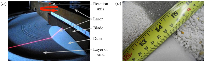
Figure 1: (a) Photo of the experimental setup. (b) Photograph of the four granular materials. From left and clockwise: aquarium sand ($d=0.9$ mm); spherical glass beads ($d=1$ mm); coarse grit ($d=3$ mm); and fine glass beads ($d=0.1$ mm).

To begin each experiment, we first poured the granular material onto the rotating table, filling up the gap underneath the blade and ploughing out a layer of constant thickness and compaction. The vertical separation of the blade from the bed avoided particles becoming jammed and crushed between the blade and the table. Although the thickness of this pre-existing layer adds to the parameters of the problem, we ran additional experiments to check that variations in its depth over the range 10–30 mm did not significantly change the observed phenomenology at the rotation rate, $\Omega=0.05$ rad s^-1. The DEM simulations in §4.3 offer further gauging of the effect of the underlying layer.

Once the pre-existing layer was in place, we stopped the table, and then slowly poured an additional mass of grains onto the layer at a selected position. This created an initial pile in the form of a nearly conical mound of given mass $m$, with a slope given by the static angle of repose of the particular granular material and centred at some initial radius $r_{0}$ from the centre of the table. For the present study, we used $r_{0}=15$, $25$ or $35$ cm, and masses of $m=250$ g, $500$ g, $750$ g and $1000$ g. The table was then set in motion again, accelerating to a prescribed rotation rate, $\Omega$, with equivalent rotation period $T_{rot}=2\pi/\Omega$, in typically less than 2 seconds (well before the pile hits the blade). The collision of the pile and the subsequent dynamics then took place at constant rotation rate.

2.2 Granular materials

In this study, we considered four different granular media, two of irregular shape and two spherical, as shown in figure 1b:

1. aquarium sand (left; manufacturer PetCo);

2. coarse grit (right);

3. $1$ mm diameter glass beads (top; A-100 from Potters Industries);

4. $0.1$ mm diameter glass beads (bottom; #8 from Kramer Industries).

The mean particle size, or their ranges, for all of the granular materials are summarized in table 1.

Granular materials are often characterized by static and dynamic angles of repose, although these have no universally agreed definitions. To estimate these for each of our four materials, we half-filled a drum of inside diameter $138$ mm and axial length $93$ cm. Rotating the drum at low speeds led to episodic avalanching punctuated by periods of rigid body rotation (the so-called “slumping” regime; e.g. GDR Midi (2004)). By fitting a line to the free surface, we then measured the average angle at which avalanches started, $\theta_{start}$, and ended, $\theta_{stop}$. Rotation of the drum at faster speeds eventually precipitated continuous avalanching (the “rolling” regime) at a dynamic angle of repose, $\theta_{c}$. For the glass ballotini and sand, the free surface remained fairly linear even at the higher rotation rates. However, the surface of the grit was significantly nonlinear during continuous avalanching, indicating that $\theta_{c}$ only roughly characterizes the slope of the entire surface for this material. These angles are listed in table 1 for the four granular materials, along with the experimentally observed angle of the avalanching dune $\theta_{M}$ (discussed in more detail in section 3.2). The data are similar to cruder measurements that we made of the surface slopes of slowly built up sandpiles (cf. Börzsönyi et al., 2008).

	$d$ / mm	$\rho$ / g cm-3	$\qquad\theta_{start}\qquad$	$\qquad\theta_{stop}\qquad$	$\theta_{c}$	$\theta_{M}$
Ballotini	$1\pm 0.2$	$1.48-1.61$	$24.9\pm 0.7\!\char 23\relax$	$22.9\pm 0.5\!\char 23\relax$	$23.7\pm 0.6\!\char 23\relax$	$23.4\pm 0.5\!^{\char 23\relax}$
Ballotini	$0.12\pm 0.03$	$1.50-1.60$	$26.6\pm 0.7\!\char 23\relax$	$23.8\pm 0.6\!\char 23\relax$	$25.3\pm 0.5\!\char 23\relax$	$23.5\pm 0.5\!^{\char 23\relax}$
Aquarium sand	$0.9\pm 0.15$	$1.50-1.67$	$37.9\pm 1.3\!\char 23\relax$	$33.7\pm 1.1\!\char 23\relax$	$36.1\pm 1.0\!\char 23\relax$	$36.1\pm 0.5\!^{\char 23\relax}$
Coarse grit	$3\pm 0.9$	$1.46-1.64$	$39.2\pm 0.9\!\char 23\relax$	$33.1\pm 0.8\!\char 23\relax$	$36.3\pm 1.5\!\char 23\relax$	$35.5\pm 0.5\!^{\char 23\relax}$

Table 1: Mean particle diameter $d$, apparent density $\rho$, and characteristic angles for the four different granular media. The mean diameter of the aquarium sand and coarse grit particles have been estimated by direct visualization and fitting a Gaussian distribution to the recorded particles sizes; the quoted error is the standard deviation (see Sauret, 2012, for more details). For the ballotini, we quote the particle range and its median as provided by the producers. The apparent densities are determined by measuring the mass of one litre of each of the materials with either loose packing or after compaction. $\theta_{start}$ and $\theta_{stop}$ denote the starting and stopping angles for avalanches in a slowly rotating drum; $\theta_{c}$ is the the dynamic avalanching angle at the initiation of the continuous flow regime in the same drum rotated at higher speed. $\theta_{M}$ is the angle of the low-rotation-rate master curves observed in the bulldozing experiments, as described in more detail in section 3.2.

2.3 Diagnostic method: calibration and topography of the dune

To describe the geometry of the bulldozed dune, we use the Cartesian coordinate system $(x,y,z)$ illustrated in figure 2. The axes are orientated so that the $z-$axis points vertically upwards with $z=0$ corresponding to the base of the bulldozer (or the surface of the underlying granular layer), the $x-$axis is perpendicular to the bulldozer blade and $y$ runs along its front face. The surface profile of the dune, $z=h(x,y,t)$, is equivalent to the local depth of material above the pre-existing granular layer. Note that, because of the finite thickness of the blade and the way that we positioned the wooden beam, the origin of the coordinate system does not coincide with the rotation axis of the table. Instead, the origin is offset from the centre of the rotating table and is positioned at the closest point along the blade.

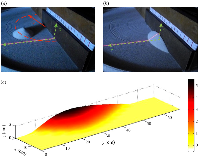
Figure 2: Coordinate system and laser measurement technique used to characterize the surface of the bulldozed pile: a Cartesian coordinate system is orientated so that the $z-$axis points vertically upwards, $x$ is perpendicular to the bulldozer’s blade and $y$ runs laterally along its front face. (a) Without topography, the laser line (red) runs along the top of the uniform underlying layer and defines a section in $x$ at $z=0$ for a particular position in $y$; the $(x,z)$ plane at this location in $y$ is shown. The dashed semi-circle indicates the radial position $r_{0}$ of the centre of the initial pile. (b) When the topography of the dune cuts through the line of the laser, the deviation from the original straight line can be used to measure the elevation of the surface, $z=h(x,y,t)$. (c) The reconstructed dune profile for a mass $m=1000$ g of $1$ mm glass beads, with rotation rate $\Omega=0.05$ rad s^-1 and initial position $r_{0}=25$ cm.

To determine the profile of a dune, we projected a laser line onto its surface, measuring the deflection away from the pre-existing layer due to that topography as shown in figure 2a,b (cf. Pouliquen, 1999a). The laser line was orientated perpendicular to the blade, and fixed on a traverse such that the laser could be swept along the length of the blade. The perpendicular profile (i.e. in an $(x,z)$-plane) of the dune could then be measured at various lateral (radial) positions along the blade. However, most of our perpendicular profile measurements were taken at the lateral location, $y_{0}\approx r_{0}$ corresponding to the position where the centre of the initial pile hits the blade. To deal with effects of perspective and projection, we first performed a calibration using images of square boards, suitably positioned in the field of view of the camera. (See Sauret (2012) for more details.) This exercise furnished the proper map between the deflections measured in the pixels of the camera and the actual distances in three-dimensional space. Figure 2c shows a typical example of the reconstruction of the entire topography of a dune.

3 Experimental results

3.1 Phenomenology

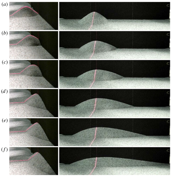
Figure 3: Successive pictures of the bulldozed dune from a side view (left) and a front view (right) for $r_{0}=25$  cm, $\Omega=0.05$ rad s^-1 and $m=1000$ g. The times of the snapshots are (a) $t/T_{rot}=0$, (b) $0.032$, (c) $0.064$, (d) $0.127$, (e) $0.24$ and (f) $0.64$. In all pictures, the laser line highlights the topography of the dune at the location $y_{0}$. Videos of these experiments are available as supplementary materials.

A collision between a conical pile of aquarium sand and the blade is illustrated in figure 3 and documented further in the videos available as supplementary material. The bulldozing dynamics takes place in two phases. The collision prompts a rapid initial rearrangement of the granular material into an avalanching dune driven primarily perpendicular to the blade (figure 3b,c). This avalanching state becomes quasi-steady in its perpendicular motion, but subsequently spreads laterally over a longer time scale (figure 3d-f). The two phases are evident in figure 4, which plots time series of the depth of the dune at the position $y_{0}$ along the blade corresponding to the initial radius of the pile, i.e. $h(0,y=r_{0},t)\equiv H(y=r_{0},t)$, for a number of different experiments. Note that we fix the origin of time, $t=0$, as the moment when the edge of the initial pile makes contact with the blade of the bulldozer.

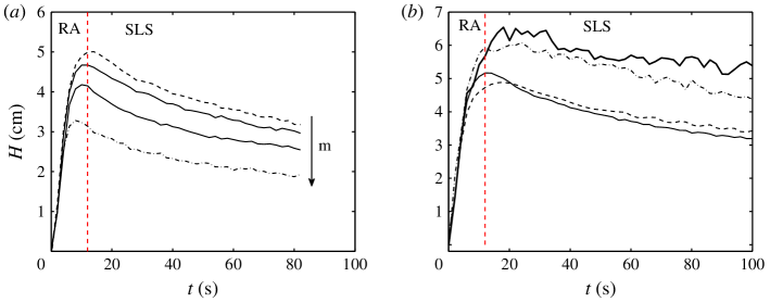
Figure 4: Time series of the depth of the dune against the blade, $h(0,y_{0},t)\equiv H(y_{0},t)$ at $y=y_{0}\approx r_{0}=25$ cm, with $\Omega=0.05$ rad s^-1, for (a) $1$ mm glass beads with varying mass ($m=250$, 500, 750 and 1000 g) with the arrow indicating decreasing initial mass; (b) the four granular materials with fixed mass $m=1000$ g (grit - thick line, aquarium sand - dashed-dotted line, $1$ mm glass beads - dashed line, $0.1$ mm glass beads - solid line). The vertical lines at $t=12$ s indicate the rough switch over from the rapid initial adjustment (labelled “RA”) to the slower lateral spreading phase (“SLS”).

The rapid adjustment phase spans a time $T_{i}$ of the order of tens of seconds, or a fraction of the rotation period. This time scale can be rationalized in terms of the characteristic length of time required to reorganize a pile of initial radius $R_{0}$ by flow with speed $U=r_{0}\,\Omega$, $T_{i}\sim R_{0}/(r_{0}\,\Omega)\approx 12\,$s (for $R_{0}\approx 15$ cm, $r_{0}\approx 25$ cm and $\Omega=0.05$ rad s^-1), which is indicated in figure 4a,b. Lateral spreading, on the other hand, takes place over a time scale $T_{q}$ spanning multiple rotations, suggesting that $T_{q}=O(T_{rot})$, which is consistent with the predictions of the depth-averaged model presented below in section 3.3.

3.2 Dynamics perpendicular to the blade

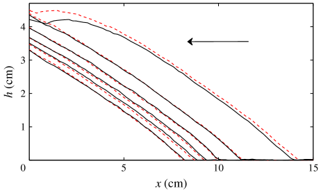
Figure 5: Profiles of two bulldozed dunes at $y=25$ cm for initial piles of $m=1$ kg of $1$ mm glass beads located at $r_{0}=25$  cm, with $\Omega=0.05$ rad s^-1. The profiles are taken every 10 seconds starting at $15$ seconds after the pile hits the blade, with the direction of increasing time being shown by the arrow. The profiles for the two distinct experiments are shown by dashed and solid lines.

We first consider the quasi-steady perpendicular profiles of the avalanching dunes at fixed lateral position $y$. Profiles from two different experiments with the aquarium sand and similar initial conditions and rotation rate ($r_{0}=25$ cm, $m=1$ kg and $\Omega=0.05$ rad s^-1) are shown in figure 5. The two earliest profiles show slight variations due to minor differences in the initial piles: although the mass is fixed, particles can be packed slightly differently (see e.g. Jaeger et al., 1996) and the exact position of the initial pile can vary by a few millimetres. These variations become less significant during the initial rapid adjustment into the quasi-steady bulldozed dune, leaving profiles that agree to within the measurement errors of the laser system, which are approximately 2 mm. The profiles then slowly reduce in height over the time scale $T_{q}$ due to lateral spreading. Thus, the evolving topography of the dune is reproducible in the experiments.

We plot quasi-steady profiles for $1$ mm glass beads in figure 6a for an initial mass $m=1000$ g. The slope of the dune remains nearly constant over the duration of the period shown, even though the perpendicular area falls by a factor of about two due to lateral spreading. Interestingly, when we scale $h(x,y,t)$ and $x$ by the depth at the blade, $h(x=0,y,t)\equiv H(y,t)$, all the profiles collapse onto a common curve, as shown in figure 6b. To leading order, this “master curve” is linear, but flattens out slightly at the blade as $x\rightarrow 0$ and steepens up near the front of the dune as $h\rightarrow 0$.

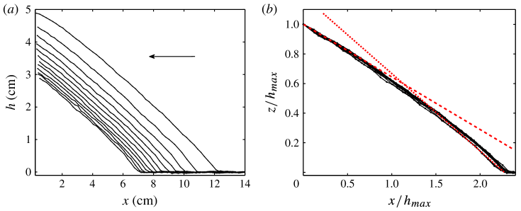
Figure 6: Perpendicular profiles at $y=y_{0}$ for a bulldozed dune of $1$ mm glass beads with $\Omega=0.05$ rad s^-1, $y_{0}\approx r_{0}=25$ cm and $m=1000$ g. Panel (a) shows plots dimensional dune profiles, $h(x,y_{0},t)$, against $x$; the profiles decay with time and are measured every $8$ seconds. Panel (b) shows the scaled profiles, $h(x,y_{0},t)/H(y_{0},t)$ against $x/H(y_{0},t)$, where $H(y,t)=h(x=0,y,t)$ is the depth against the blade. The dotted line shows the local slope at $x=0$, and the dashed line is the local slope at the flow front (as $h\rightarrow 0$).

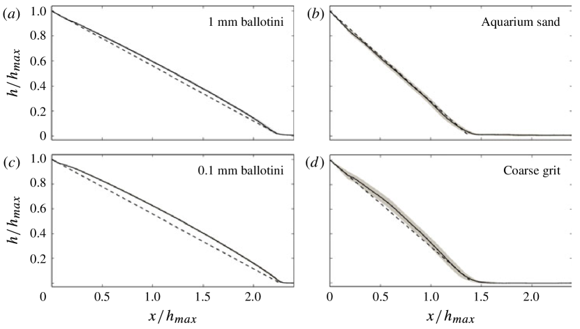
Figure 7: Master curves for: (a) $1$ mm glass beads; (b) aquarium sand; (c) $0.1$ mm glass beads; (d) coarse grit with, $\Omega=0.05$ rad s^-1, $r_{0}=25$ cm and $m=1000$ g. The master curves are constructed by averaging between 10 and 15 scaled perpendicular profiles at $y=y_{0}\approx r_{0}$ (see figure 6) taken every 4 s. The grey band shows the standard deviation of the scaled profiles about the mean master curve. The dashed line linearly interpolates between the blade and the tip of the dune.

Figure 7 shows master curves (constructed by averaging between ten and fifteen profiles taken every four seconds after the dune converges to its quasi-steady state) for our four granular materials with $\Omega=0.05$ rad s^-1, $r_{0}=25$ cm and $m=1000$ g. In the figure, the grey band indicates the standard deviation of the profiles about the average. For the glass beads, the profiles all collapse closely to the master curve (the corresponding grey bands are relatively thin), while there are more significant variations about the average for the irregularly shaped sand and grit particles. The dashed lines in the figure indicate the leading-order slopes of the master curves, obtained by linearly interpolating between the intersection of the master curve with the blade and the front of the dune. The angles corresponding to these slopes, which we denote by $\theta_{M}$, are similar to the dynamic avalanching angles $\theta_{c}$ measured in the rotating drum, as reported in table 1. Although the master curves are mostly linear, there is some curvature to these profiles, particularly for the glass ballotini, suggesting an interesting effect of particle shape.

In figures 8a–d, we plot master curves constructed from experiments with varying initial mass $m$ and radial position $r_{0}$, for both 1 mm glass beads and aquarium sand. For each material, the various experiments collapse onto the same master curve. Similarly, when we take measurements of the perpendicular profiles of the bulldozed dunes at different radial positions $y$ along the blade, we also recover a common master curve. Only when we significantly speed up the rotation of the table do we observe any change in the characteristic structure of the master curves. As illustrated in figures 9a,b, when the angular velocity $\Omega$ is increased, the curves become more nonlinear, somewhat similarly to the fashion in which the surface of flow in granular drums develops a characteristic ‘S-shape’ GDR Midi (2004); Taberlet et al. (2006).

Figure 8: Master curves with $\Omega=0.05$ rad s^-1 at $y=y_{0}\approx r_{0}$ for: (a) $r_{0}=25$ cm and various initial mass ($m=250$, 500, 750, 1000 g) for $1$ mm glass beads; (b) $m=1000$ g and varying initial position ($r_{0}=15$, 25 and 35 cm) for $1$ mm glass beads; (c) $r_{0}=25$ cm and various initial mass ($m=250$, 500, 750, 1000 g) for aquarium sand; (d) $m=1000$ g and varying initial position ($r_{0}=15$, 25 and 35 cm) for aquarium sand.

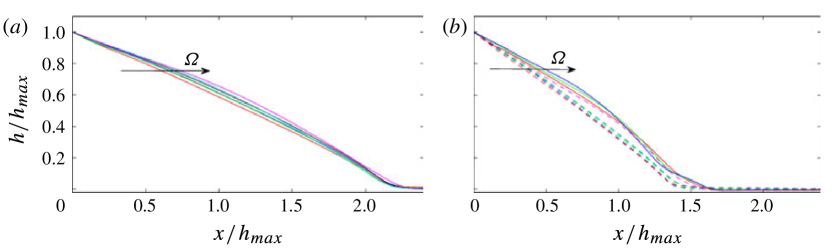
Figure 9: Master curves with $m=1000$ g at $y=y_{0}\approx r_{0}=25$cm and different rotation rate, for (a) $1$ mm glass beads ($\Omega=0.05$, $0.1$, $0.2$, $0.4$, $0.8$ and 1 rad s^-1); (b) aquarium sand ($\Omega=0.05$, $0.2$, $0.4$ rad s^-1 - dashed, and $\Omega=0.8$, $1$, $1.5$, $2$ rad s^-1 - solid). The arrows indicates the direction of increasing $\Omega$.

More generally, one would expect that the speed dependence of the master curves would arise through the local Froude number, $\mathrm{Fr}=|U_{b}|/\sqrt{gH}\equiv y\Omega/\sqrt{gH}$, where $|U_{b}|$ is the speed of the bulldozer. The experiments in figures 6-8 are conducted at relatively low Froude number, $\mathrm{Fr}=O(10^{-2})$ or less, and so the dependence on the radial position, $y$, and the depth at the blade, $H$, is not evident; the curves in these figures characterize the zero-Froude-number limit. Only when the rotation rate is increased by two orders of magnitude, as in figure 9, does the Froude-number dependence become apparent. In any event, we conclude that the perpendicular profiles collapse to Froude-number-dependent master curves that are characteristic of the granular material, much as the shape of the free surface reflects the flow dynamics in a rotating granular drum.

A final noteworthy point is that the perpendicular avalanching was always observed to be steady, except over the longer time scale of lateral spreading. This contrasts with what one observes in rotating drums, wherein flows become intermittent at low rotation rates and occur via episodic avalanching. In fact, our DEM simulations did show intermittent motion at low bulldozing speed (see §4.3), with avalanching becoming temporally irregular, if not episodic. Thus, our experiments were probably not conducted at sufficiently low speeds to observe unsteady states.

3.3 Lateral spreading of the dune

In addition to the quasi-steady perpendicular profile, the rearrangement of the granular mound prompted by the collision of the initial conical pile with the bulldozer also generates a distinctive lateral profile, $H(y,t)=h(0,y,t)$, along the blade. Figure 10 displays the spreading of this lateral profile for 1 mm ballotini. Initially, the collision establishes a shape that is almost mirror symmetric in $y$ about the centre of the initial pile, $y=y_{0}\approx r_{0}$. The dune subsequently spreads both inwards, towards the centre of the rotating table, and outwards to larger radii. The rate of spreading is, however, asymmetrical, with the dune spreading faster at larger radii and the inward edge eventually coming to rest at a finite distance from the centre of the table. This asymmetry results in part from the increase of the perpendicular velocity ${U_{b}}=-\Omega\,y$ with radial position $y$. However, because the front of the blade is positioned at a small distance $\delta$ in front of the centre of the rotating table, there is an additional tangential velocity along the blade, ${V_{b}}=\Omega\,\delta$, which advects the dune radially outwards (cf. §4.2).

Figure 10: Lateral profiles, $H(y,t)=h(x=0,y,t)$, for $1$mm glass beads with $\Omega=0.05$ rad s^-1, $m=1000$ g, and initial position $r_{0}=25$ cm. The arrows indicate the direction of increasing time and the profiles are taken every $5$ seconds after the dune hits the blade.

In figure 11, we plot the evolution of the lateral profile for dunes of aquarium sand for different initial positions $r_{0}$; the lateral spreading depends significantly upon the value of $r_{0}$. In all three cases, the dune spreads in the same asymmetrical fashion. However, unlike for the perpendicular profiles discussed earlier, there appears to be no straightforward scaling that collapses all these data. Similarly, we are unable to collapse the lateral profiles of dunes with different initial masses; only from a more qualitative perspective are the different experiments comparable. Likewise, lateral spreading is qualitatively, but not quantitatively, similar for the other granular material (cf. figure 10).

Figure 11: Lateral profiles $H(y,t)=h(x=0,y,t)$ for aquarium sand with $\Omega=0.05$ rad s^-1, $m=1000$ g, and varying initial position: (a) $r_{0}=15$ cm, (b) $r_{0}=25$ cm and (c) $r_{0}=35$ cm. The arrows indicate the direction of increasing time and the profiles are taken every $5$ seconds after the dune hits the blade.

Nevertheless, data from experiments with the same initial mass and position but different rotation rate can be conveniently collapsed, as illustrated in figure 12. Time series of the locations of the inner and outer edges, denoted by $y_{-}(t)$ and $y_{+}(t)$, are plotted for the 1 mm glass beads and the aquarium sand. Also shown is the time series of the maximum depth of the dune against the blade, $H_{max}(t)={\rm Max}_{y}\{H(y,t)\}$, along with the radial location $y_{max}(t)$ at which that maximum occurs. By plotting these quantities against the dimensionless time $\Omega\,t$, the data collapse, confirming that the rotation rate controls the spreading dynamics.

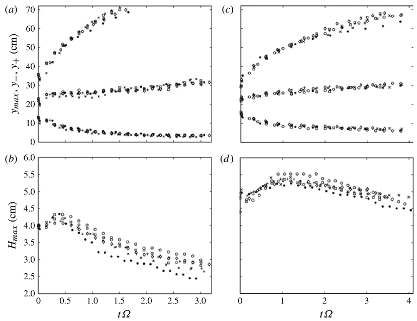
Figure 12: Time series of (a,c) the locations along the blade of the inner and outer edges of dunes, $y_{-}$ and $y_{+}$ and the position of maximum depth, $y_{max}$, and (b,d) the maximum depth, $H_{max}={\rm Max}_{y}\{H(y,t)\}$. The results are plotted against $\Omega t$ for different rotation rates ($\Omega=0.05$ rad s^-1 - $\circ$, $0.1$ rad s^-1 - $\square$, $0.2$ rad s^-1 - $+$, $0.4$ rad s^-1 - $\diamond$, $0.8$ rad s^-1 - $\times$ and 1 rad s^-1 - dots). All the piles have $m=1000$ g and $r_{0}=25$cm. In (a,b), data for 1 mm ballotini are shown; (c,d) show data for aquarium sand.

Lateral spreading also appears to be insensitive to the initial shape of the dune, as we found in other experiments in which grains of aquarium sand were deposited in half-cones propped up against the blade before rotating the table; once rotation began, the profiles spread laterally and quickly became very similar to those recorded for the full sandpiles that suffered collisions against the blade. This insensitivity suggests a scaling of the lateral profiles based on the depth-averaged model of §4.2. According to this model, if we scale the lateral position by $y_{0}$ and the profile by a characteristic depth $H_{0}=\sqrt{2\mu V/y_{0}}$, then experiments with comparable values of the parameter $C=\mu\delta/H_{0}$ should be similar at the scaled time $t/t_{0}$, with $t_{0}=\mu y_{0}/\Omega H_{0}$. Here, $V$ is the initial volume (estimated as $m/\rho$, with $\rho$ the average of the loose and compacted apparent densities listed in table 1) and $\mu\equiv\mu_{M}$ is the leading-order perpendicular slope. The scaling is illustrated in figure 13 for three of the $1$ mm ballotini experiments with $C\approx 0.2$). The comparison is marred to begin with by the transient during which the memory of the detailed initial shape is destroyed. Beyond that transient, however, the scaled profiles do appear to follow a common evolution (at least until the dune is swept out to the edge of the table). Figure 13 also includes data from one of the aquarium sand experiments (again with $C\approx 0.2$); although the comparison of the scaled data is less satisfying than for the ballotini, the scaling enjoys some success in view of the relatively large differences in the unscaled data.

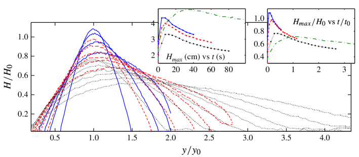
Figure 13: Scaled lateral profiles for 1 mm ballotini. In the main panel, lateral position $y$ is scaled by the initial position $y_{0}$, and depth by $H_{0}=\sqrt{2\mu V/y_{0}}$, where $V$ is the initial volume (based on the deposited mass $m$ and the average apparent density listed in table 1). Three different experiments are shown with $(m,y_{0})=$($500\,$g, $15\,$cm) (dotted), ($750\,$g, $25\,$cm) (dashed) and ($1000\,$g, $35\,$cm) (solid). The left-hand inset shows the maximum depth against time; in the right-hand inset, the data is scaled, plotting $H/H_{0}$ against $t/t_{0}$, with $t_{0}=\mu\,y_{0}/\Omega H_{0}$. Data from an experiment with aquarium sand and $(m,y_{0})=$($750\,$g, $15\,$cm) is also included in the insets (dot-dashed).

4 Theoretical models

To parallel our experimental discussion, we now provide two versions of a simple depth-averaged model designed to examine quasi-steady perpendicular avalanching and lateral spreading. We then present DEM simulations of a slightly simpler arrangement, the planar bulldozer (i.e. granular dunes driven forwards by a vertical plate undergoing rectilinear motion), addressing some of the limitations of the depth-averaged models.

4.1 A depth-averaged model for the perpendicular profile

Depth-averaged models are a conventional tool to analyse shallow, incompressible granular flows (Savage & Hutter 1991; Forterre & Pouliquen 2008; Andreotti, Forterre & Pouliquen 2013). In two dimensions and for steady flow over a horizontal plane, the depth-integrated equations expressing conservation of mass and horizontal momentum are

$$\frac{\partial}{\partial x}\left(\int_{-b}^{h}u\,\,\text{d}z\right)=0\qquad{\rm and}\qquad\rho\,\frac{\partial}{\partial x}\left(\int_{-b}^{h}u^{2}\,\,\text{d}z\right)=\frac{\partial}{\partial x}\left(\int_{-b}^{h}\sigma_{xx}\,\,\text{d}z\right)-\mu_{b}\,p(x,-b),$$ (1)

where $u(x,z)$ denotes the horizontal velocity, the underlying plane is positioned at $z=-b$ (the base of the blade of the bulldozer being located at $z=0$) and $\rho$ is the density. Here, the normal stresses are $(\sigma_{xx},\sigma_{zz})$ and the shear stress on the base of the layer is expressed as a product of the isotropic pressure $p(x,z)$ and a friction coefficient $\mu_{b}$. For shallow flow, hydrostatic balance typically prevails in the vertical direction and the pressure dominates the normal stresses,

$$\sigma_{xx}\approx\sigma_{zz}\approx-p\approx-\rho g(h-z),$$ (2)

where $g$ is gravity and we ignore the atmospheric pressure above the granular layer.

The first relation in (1) indicates that the horizontal flux is uniform, which, in view of the upstream conditions, implies

$$\int_{-b}^{h}u\,\,\text{d}z=b\,{U_{b}}.$$ (3)

To deal with the second relation, we require expressions for the local vertical profile of the velocity and $\mu_{b}$. For the former we adopt the Bagnold form (e.g. Andreotti et al., 2013),

$$u(z)={U_{b}}-\frac{5\,h\,{U_{b}}}{3\,(h+b)^{5/2}}\,[(h+b)^{3/2}-(h-z)^{3/2}].$$ (4)

Here, the flow is described in the frame of the bulldozer, wherein ${U_{b}}$ is the speed of the underlying table, which is equal and opposite to the speed of the bulldozer (for our rotating table, $U_{b}=-\Omega\,y$). For the basal friction coefficient, the local $\mu(I)$ rheology proposed by GDR Midi (2004) suggests that $\mu_{b}$ is a function of an “inertia number”

$$I=\frac{5\,d\,h|{U_{b}}|}{2\,\sqrt{g}\,(h+b)^{5/2}}$$ (5)

(the local basal shear rate being $5h|{U_{b}}|/2(h+b)^{2}$), where $d$ is the particle diameter. A convenient explicit expression for the $I$ dependence of the friction is

$$\mu_{b}(I)=\mu_{1}+(\mu_{2}-\mu_{1})\frac{I}{I_{0}+I},$$ (6)

for three material constants $\mu_{1}$, $\mu_{2}$ and $I_{0}$ Jop et al. (2006).

The preceding formulae can be combined into a single expression for the local slope of the free surface,

$$\frac{\partial h}{\partial x}=-\mu(I)\left\{1+\frac{{U_{b}}^{2}}{4\,g\,(h+b)}\left[1-\frac{5\,b^{2}}{(h+b)^{2}}\right]\right\}^{-1},$$ (7)

and the profile can be computed using quadrature. For 1 mm glass beads with $\mu_{1}=\tan 21^{\circ}$, $\mu_{2}=\tan 30^{\circ}$ and $I_{0}=0.3$, and the experimental parameters given in figure 9, we find the profiles shown in figure 14. Apart near the front edge, the free surface has a slope close to $\mu_{1}$. Closer to the front, the shape depends on the depth of the incoming layer, $b$, and the local Froude number $U_{b}/\sqrt{g(h+b)}$. For bulldozing on a “dry” plane ($b=0$) and relatively slow flows with $U_{b}/\sqrt{g\,h}\ll 1$, the front steepens up to a “contact angle”, $\tan^{-1}\mu_{2}$ (cf. Pouliquen, 1999a). With inertia however, i.e. $U_{b}/\sqrt{g\,h}=O(1)$, material is pushed out ahead of the main wedge, creating a distinctive forward skirt. The situation is quite different when there is an incoming layer, $b>0$: the factor $1-5\,b^{2}/(h+b)^{2}$ reverses the sign of the inertial correction near the front, with the result that the wedge steepens further there, and even becomes vertical if the bulldozing speed is increased beyond $\sqrt{g\,b}$, suggesting that the front overturns and breaks.

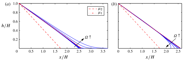
Figure 14: Perpendicular profiles computed from (7) assuming $\mu_{1}=\tan 21^{\circ}$, $\mu_{2}=\tan 30^{\circ}$, $I_{0}=0.3$, $k=1$, $h(0)=H=5$ cm, $r_{0}=25$ cm and the same rotation rates as in figure 9, i.e. $\Omega=0.05,0.1,0.2,0.4,0.8,1,1.5$ and $2$ rad s^-1. In (a) $b=0$; in (b) $b=2$  cm.

Although the depth-averaged model predicts that the profile is nearly linear with a front that steepens with an increase in rotation rate, much as in the experiments, the finer details of the measured profiles are not reproduced (such as the flattening of the profile at the blade). In fact, it is surprising that the model looks to work better for the sand than the ballotini, despite the fact that the $\mu$($I$) model is designed for the latter and is known to require revision for sand (e.g. Forterre & Pouliquen, 2008). Part of the problem is that the depth-averaged model discards horizontal derivatives, with the consequence that there are sudden switches in the flow pattern at the junction of the wedge with the incoming layer and at the bulldozing plate. More properly, boundary layers should be introduced at these locations to provide smoother connections. As is clear from the DEM simulations described later, the assumption that the vertical flow profile takes the Bagnold form in (4) can also be suspect, with the flow adjusting more gradually from the incoming plug to the recirculating wedge. Moreover, the DEM simulations reveal interesting variations in the packing fraction, which may impact the local rheology, whereas the model is incompressible.

4.2 Lateral spreading

To construct a simple model of lateral spreading, we couple the depth-averaged mass conservation equation with some approximations suggested by the observation that flow becomes quasi-steady perpendicular to the blade. For simplicity, we also ignore any motion in the uniform layer flowing underneath the blade (i.e. in $z<0$). Conservation of mass then implies

$$\frac{\partial h}{\partial t}+\frac{\partial}{\partial x}\left(\int_{0}^{h}u\,\text{d}z\right)+\frac{\partial}{\partial y}\left(\int_{0}^{h}v\,\text{d}z\right)=0,$$ (8)

where $\left(u(x,y,z,t),v(x,y,z,t)\right)$ denotes the horizontal velocity field. We rewrite this equation as

$$\frac{\partial h}{\partial t}+\frac{\partial}{\partial x}(h\,{U_{b}}+F_{x})+\frac{\partial}{\partial y}(h\,{V_{b}}+F_{y})=0,$$ (9)

where $\left({U_{b}},{V_{b}}\right)$ is the velocity of the underlying layer in the reference frame of the blade and

$$(F_{x},F_{y})\equiv\int_{0}^{h}(u-{U_{b}},v-{V_{b}})\,\text{d}z$$ (10)

denotes the flux due to the avalanching internal motion of the granular material.

As discussed above, the granular flow in the transverse $x$-direction adjusts relatively quickly and the bulldozed dune becomes quasi-steady. Therefore, the net transverse flux in (9), namely $h\,{U_{b}}+F_{x}$, must become small,

$$F_{x}\approx-h\,{U_{b}}.$$ (11)

Any residual transverse flux balances the slow time variation of $h$ and the weaker lateral flux along the blade. Nevertheless, that residual flux must vanish exactly at both the blade and the leading front $x=X(y,t)$ of the dune, and so $[h\,{U_{b}}+F_{x}]_{x=0}=[F_{x}]_{x={X}}=0$. Hence, to model lateral spreading, whilst avoiding the need to construct the residual transverse flux, we integrate (9) over the $x$-direction to obtain the relation

$$\frac{\partial}{\partial t}\left(\int_{0}^{{X}}\,h\,\,\text{d}x\right)+\frac{\partial}{\partial y}\int_{0}^{{X}}\,(h\,{V_{b}}+F_{y})\,\,\text{d}x=0.$$ (12)

We now exploit the fact that the transverse profile of the dune is almost linear,

$$h(x,y,t)\approx H(y,t)-\mu\,x,$$ (13)

with constant slope, $\mu$. Hence $X(y,t)=H(y,t)/\mu$. Furthermore, for a free-surface gravity-driven flow, one would expect that the avalanche flux, $(F_{x},F_{y})$, would be directed downslope, i.e. $\mathbf{F}\approx-\Gamma\nabla h$, where the factor $\Gamma$ encapsulates the detailed physics of the granular flow. Hence,

$$F_{y}\approx F_{x}\,\frac{h_{y}}{h_{x}}\approx\frac{h\,{U_{b}}\,H_{y}}{\mu}$$ (14)

using (11) and (13). Thus,

$$\frac{1}{2\mu}\frac{\partial H^{2}}{\partial t}+\frac{\partial}{\partial y}\int_{0}^{{{X}}}\,(H-\mu x)\left({V_{b}}+\frac{{U_{b}}\,H_{y}}{\mu}\right)\,\,\text{d}x=0.$$ (15)

Once the basal velocity, $({U_{b}},{V_{b}})$, is prescribed, the integral in (15) can be computed and the model can be completed.

4.2.1 The planar bulldozer

When the bulldozer undergoes rectilinear motion in the $x-$direction, ${V_{b}}=0$ and $U_{b}$ is a constant that must be negative if the blade is located at $x=0$ and the wedge is piled up in $x>0$. Equation (15) then reduces to

$$\left(H^{2}\right)_{t}=-\frac{{U_{b}}}{\mu}\left(H^{2}H_{y}\right)_{y}.$$ (16)

As illustrated in figure 15, we may solve (16) as an initial-value problem given a suitable initial condition (a Gaussian in the figure). Over longer time, the numerical solution converges to a similarity solution given by

$$H(y,t)=\left\{\begin{array}[]{lc}H_{max}(1-y^{2}/Y^{2}),&{\rm for}\ -Y<y<Y,\cr 0,&{\rm elsewhere,}\end{array}\right.$$ (17)

where

$$Y(t)=\left(\frac{375\,V\,{U_{b}}^{2}\,t^{2}}{8\,\mu}\right)^{1/5},\qquad H_{max}(t)=\left(\frac{45\,\mu^{3}\,V^{2}}{64\,t\;|{U_{b}}|}\right)^{1/5}.$$ (18)

and $V\equiv\int H^{2}\text{d}y/2\mu$ is the volume of grains in the dune. Solutions beginning with a wide range of single-humped initial conditions converge to the self-similar form in (17). In other words, after a transient that obliterates the initial shape, the mound adopts a characteristic parabolic profile, spreading laterally like $t^{2/5}$ while its maximum depth falls like $t^{-1/5}$.

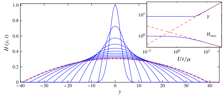
Figure 15: Solution to the planar bulldozer problem defined by (16), showing the collapse of a Gaussian, $H(y,0)=e^{-y^{2}/10}+10^{-4}$, towards the similarity solution in (17)-(18) (red dots and dashed lines). The main panels shows ten snapshots of the solution, equally spaced in $t^{2}$ up to $t=10^{3}\mu/|{U_{b}}|$; the inset shows the maximum depth $H_{max}(t)$ and edge position $Y(t)$. The pre-wetted film of depth $10^{-4}$ is added to avoid any numerical problems with the vanishing of the diffusivity in (16), and is sufficiently shallow that it has no effect on the solution. For the numerical solution, the edges of the dune, $y=\pm Y(t)$, are defined as the positions where $H(y,t)=2\times 10^{-4}$.

4.2.2 The rotating bulldozer

In our Cartesian coordinate system, the front face of the blade lies along the $(y,z)-$plane at $x=0$. However, as already noted, in our experiments the rotation axis was offset from the origin of the coordinate system by a distance $\delta$. The basal velocity field is then U_b& = -Ω y,
V_b = Ω (x+δ) (the rotation axis being located along the line $(x,y,z)=(-\delta,0,z)$). Thus,

$$\frac{\mu}{\Omega}\frac{\partial H^{2}}{\partial t}+\mu\,\delta\,\frac{\partial H^{2}}{\partial y}=\frac{1}{3}\left[y^{2}\left(\frac{H^{3}}{y}\right)_{y}\right]_{y}.$$ (19)

It should be noted that (19) applies only for $y>0$; for $y<0$, the granular medium must be piled up on the opposite side of the blade, which calls for some key switches of sign in the formulae.

We first consider the case when the blade is positioned exactly along a diameter of the rotating table, so that $\delta=0$. Numerical solutions to the corresponding initial-value problem illustrate how the dune slumps preferentially radially outwards; see figure 16, which shows the lateral spreading of an initially parabolic mound. The granular material also piles up towards the centre, building up a sharp edge near $y=0$. Again the solution converges to a self-similar solution, this time given by

$$H=\left\{\begin{array}[]{lc}\mu\,t^{-1}\,\Omega^{-1}\,y^{1/3}\,(Y^{2/3}-y^{2/3}),&0<y<Y,\cr 0,&{\rm elsewhere},\end{array}\right.$$ (20)

where

$$Y=\left(\frac{105\,t^{2}\,V\,\Omega^{2}}{4\,\mu}\right)^{1/3}$$ (21)

denotes the lateral extent of the dune, in terms of which the maximum depth and its location are given by

$$H_{max}=\frac{2\,\mu Y}{3\sqrt{3}\;t\,\Omega}\qquad{\rm and}\qquad y_{max}=\frac{Y}{3\sqrt{3}}.$$ (22)

Evidently, the linear rise of the rotation speed with $y$ increases the rate at which the dune is swept outwards and thins ($Y\sim t^{2/3}$ and $H_{max}\sim t^{-1/3}$ rather than $t^{2/5}$ and $t^{-1/5}$, respectively, for the planar bulldozer).

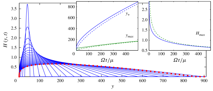
Figure 16: Numerical solution to the rotating bulldozer problem in (19) without radial advection ($\delta=0$), showing the collapse of a parabolic mound (again supplemented by a thin pre-wetted film of depth $10^{-4}$) towards the similarity solution in (20)-(21) (red dots and dashed lines). The main panels shows twenty snapshots of the solution, equally spaced in $t^{2}$ up to $t=500\mu/\Omega$; the insets show the position of the right-hand edge of the dune, $y_{+}$, the location of the maximum depth, $y_{max}$, and that depth, $H_{max}(t)$. For the numerical solution, $y_{+}$ is defined by $H(y_{+},t)=2\times 10^{-4}$.

When $\delta\neq 0$, the flux along the blade picks up an additional component that helps to sweep the dune out to larger radii, where rotational bulldozing effects a rapid diffusion to flatten out the mound. The additional advection prevents material from piling up towards the centre of the rotating table, and the solution no longer converges to the similarity solution (20) and (21). The dynamics is illustrated by the solutions of the initial-value problem shown in figure 17. These examples use parameter settings based on the experiment with aquarium sand shown in figure 17 ($\delta=2$ cm and $\mu=\tan\theta_{M}\approx\tan 36^{\circ}$), and use three different initial profiles $H(y,0)$, all with the same volume. The first is a profile obtained by taking a sandpile with slope $\mu_{s}\approx\tan 33^{\circ}$ centred at $y_{0}$ and then rearranging the material at each $y$ into wedges with slope $\mu$; this is the theoretical initial condition corresponding to the experiment given our assumption of a relatively rapid adjustment to a quasi-steady state of perpendicular avalanching. The second initial profile is also based on rearranging the sandpile. However, the simplest rearrangement of this sort furnishes an initial shape with slopes that exceed $\mu$, which would presumably avalanche laterally; to avoid this detail, the steeper slopes of the rearranged sandpile are replaced with linear sections of slope $\mu$, and the entire profile then rescaled to furnish the correct volume. The third initial condition is simply a triangle with slopes of $\mu$. As can be seen in the figure, after a short transient (lasting less than 10 seconds), all three cases converge to the same spreading solution. Thus, the finer details of the initial profile are not significant, as found experimentally.

Qualitatively, the solutions in figure 17 are similar to the experimental observations. However, although the theory rationalizes the collapse of the experimental data in figure 12 for different rotation rates, the agreement between the model and the experiment is not quantitative. This is shown in the insets of figure 17, which compare the theoretical predictions for the positions of the edges and maximum of the dune and its maximum depth with data from the experiment in figure 11b.

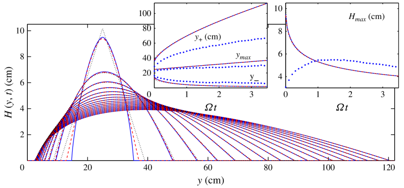
Figure 17: Numerical solution to (19) with $\Omega=0.05$ rad s^-1, $y_{0}=25$ cm, $\mu=\tan 36^{\circ}$ and $\delta=2$ cm. The snapshots of $H(y,t)$ are shown every 5 seconds, and the insets show the positions of the dune’s maximum $y_{max}(t)$, the edges of the dune $y_{\pm}(t)$, and the maximum depth $H_{max}(t)$. Three solutions are shown, starting from three different initial conditions but all with the same mass: a triangle (dotted), the profile expected from rearranging a sandpile (solid) and the profile obtained when the rearranged sandpile is adjusted to limit its maximum slope (dashed), as described further in the main text. In each case, a pre-wetted film of depth $10^{-4}$ is added and the edges are defined as the locations where $h(y,t)=2\times 10^{-4}$. The dots in the insets show the corresponding data from the experiment in figure 11b.

The insensitivity to initial shape suggests a convenient rescaling of (19). If we set

$$\hat{y}=\frac{y}{y_{0}},\qquad\hat{H}=\frac{H}{H_{0}},\qquad\hat{t}=\frac{t}{t_{0}},\qquad H_{0}=\sqrt{\frac{2\mu V}{y_{0}}}\qquad{\rm and}\qquad t_{0}=\frac{\mu\,y_{0}}{\Omega\,H_{0}},$$ (23)

then the evolution equation becomes

$$\frac{\partial\hat{H}^{2}}{\partial\hat{t}}+C\,\frac{\partial\hat{H}^{2}}{\partial\hat{y}}=\frac{1}{3}\left[\hat{y}^{2}\left(\frac{\hat{H}^{3}}{\hat{y}}\right)_{\hat{y}}\right]_{\hat{y}}$$ (24)

and the rescaled volume constraint is $\int\hat{H}^{2}{\rm d}\hat{y}=1$. Thus, the later-time solutions depend on the single parameter $C$, as was roughly confirmed experimentally in §3.3.

4.3 DEM simulations

For our DEM simulations, we used identical deformable, spherical particles. All variables are expressed in dimensionless form, with lengths scaled by the particle radius $d/2$, speeds by $\sqrt{g\,d/2}$ and times by $\sqrt{d/2g}$. Particle collisions are dealt with using a soft-particle model with a damped linear spring for the normal force (with zero coefficient of restitution) and dynamic Coulomb friction for the tangential force (with a coefficient of friction equal to 0.3). The particle stiffness was chosen so that any overlap would not exceed 1%. The time step was one tenth of the binary collision time; additional computations with a smaller time step verified the insensitivity of the results to this choice. Simulations were also performed with different stiffness values and with a static friction model wherein the tangential displacement of each contact was tracked; there was no discernible change in the main characteristics of the dunes.

To mimic the sandpaper glued to the surfaces of the experimental bulldozer and the rotating table, we suitably positioned a set of immobile particles to create a rigid vertical plate and translating underlying plane. To help prevent the particles from crystallizing against these boundaries, the immobile particles were placed on a rectangular grid with a spacing equal to $\Delta=3(2+\sqrt{3})/5$ times the particle radius. We performed two suites of computations: in one, the base of the bulldozing plate was located 20 particle radii above the plane; for the other, the base of the blade was placed next to the plane to avoid any gap between the two obstructions. In the latter, particles do become temporarily jammed between the bulldozer and the surface (the effect we sought to avoid in the experiments by emplacing the underlying layer); when released, these grains gain significant kinetic energy and can become launched out on ballistic trajectories. This dynamics depends on the model for particle collision but does not affect the overall behaviour of the dunes.

Unlike the rotational geometry of the experiment, the DEM simulations were conducted with a bulldozing plate undergoing rectilinear perpendicular motion in Cartesian geometry. We used two configurations. First, to explore the perpendicular dynamics independently of any lateral spreading, we used a relatively narrow slot with a perpendicular length of $150\Delta$ and a lateral width of $5\Delta$ (corresponding to about 150 by 6 particles). The domain was taken to be periodic in both horizontal directions, and 20 000 or 10 000 particles were released, depending on whether there was an underlying layer or not. The narrowness of the slot eliminates coherent lateral motion, and simulations in domains of different width suggested little dependence on that dimension. In our initial simulations, the particles were deposited in a triangular wedge; the ensuing bulldozing flow led to a vigorous adjustment, with a fraction of the particles launched away from the bulk on ballistic trajectories. The material took some time to settle down after this transient (requiring several passes of the blade through the domain to allow the wedge to adjust and the packing in the bed to increase). In subsequent simulations, we therefore used the particles positioned from an earlier evolved solution with a different bulldozer speed.

Second, to study lateral spreading, we prepared a much wider simulation by assembling several side-by-side copies of one of the narrow simulations and evolved this configuration for a while to reduce any spatial correlations. We then formed a localized mound against the blade in the centre of this domain by taking the profile along the midline $y=0$ and rotating this curve about the origin, clipping all the overlying particles. This created a half-cone above the bed (as can be seen in the left panel in figure 21) and minimized any subsequent vigorous adjustment. The width of the computational domain (i.e. the number of copies of the original slot) was chosen to be sufficiently large compared with the half-cone so that mobilized particles did not reach the lateral boundaries, thus rendering irrelevant the precise width and the lateral boundary conditions. Altogether, there were about $1.2$ million particles in the lateral spreading simulations with an underlying layer and about 180 000 particles in the simulations without one.

4.3.1 Dynamics of perpendicular avalanching

In our dimensionless units and with a fixed number of particles, there is only a single parameter in the simulations, which is the bulldozer speed $|U_{b}|$. During bulldozing, the particles become distributed so that they build up a wedge of depth $H$ against the blade, furnishing the effective Froude number of the flow, $|U_{b}|/\sqrt{H}$. Our main interest is in characterizing the steady flow states, so we omit any discussion of the initial transients (which can be seen in the movies in the supplementary material). Nevertheless, the nature and existence of a steady flow state is not straightforward. At the lowest Froude number, the flow becomes more intermittent in time. At higher speeds, flow patterns can also vary over very long time periods (hundreds of passes of the bulldozer). These variations can be due to small increases in the packing fraction in the basal layer and the dune, which can lead to flows with much larger fluctuations in the forces and velocities. This is presumably the same effect as seen by Gravish et al. (2010) in experiments with over consolidated packings. Moreover, despite our efforts to avoid crystallization, arrangements of perfectly close-packed grains can form adjacent to the blade and generate long-time-scale variability, as described below. Nonetheless, these problems do not substantially affect the results we present and do not mar our lateral spreading simulations.

The results of simulations at speed $|U_{b}|=1$ with and without the underlying layer are displayed in figure 18. The steady-state flow patterns within the wedges built up against the blade are shown; the superposed density plots display the packing fraction and the insets show snapshots of the particle positions colour-coded by their location at a given time earlier. Also indicated are a selection of vertical profiles of the horizontal velocity. In figure 18(a), for the simulation with an underlying layer, the wedge is about 30 particles high, which is a little more than in the largest ballotini experiment. In agreement with the experiments, the wedge has almost constant slope, flattening out near the blade and steepening near the flow front. The simulation without an underlying layer in figure 18(b) furnishes a wedge that is even flatter at the blade and steeper at its front, illustrating how the underlying layer influences the shape of the free surface. The recirculation cell within the wedge is also very different. The vertical profiles of the horizontal velocity are fairly well reproduced by the Bagnold profile in the case without an underlying layer, but the comparison is poorer when the layer is present. For either case, the vertical shear is finite at the surface, unlike that predicted by the Bagnold profile. One should note the weak backflow underneath the blade in figure 18(a).

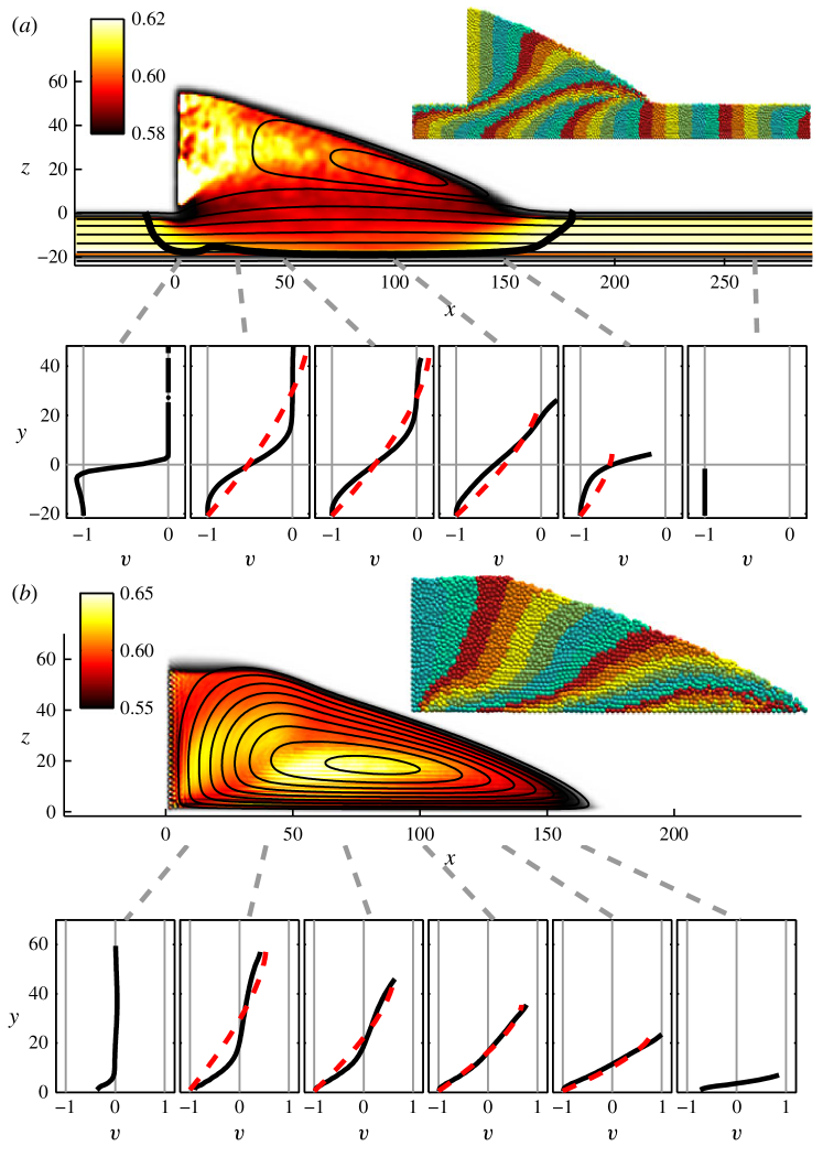
Figure 18: The steady-state flow pattern set up in simulations in the narrow slot for $|U_{b}|=1$ with an underlying layer in (a) and without one in (b). The black lines in the main panels show a selection of streamlines (not equally spaced); superposed is the packing fraction, plotted as a density on the $(x,z)-$plane. At the horizontal positions $x$ indicated, the vertical profile of the horizontal velocity $u$ is plotted in the sequence of panels underneath; the dashed lines show corresponding Bagnold profiles. The insets show snapshots of the particle distribution, with particles colour-coded according to their horizontal position $T$ time units earlier; in (a) T=100, whereas T=50 in (b). (A movie of the simulation without an underlying layer is available as supplementary material).

The “yield surface” that divides the deforming wedge from the “plug” flow in the layers in front and behind is also shown in figure 18(a). For this simulation, there is a weakly deforming triangular region propped up against the bulldozer which can be identified by an irregular pattern in the packing fraction. The weak deformation is revealed by the undeformed vertical stripes in the colour-coded particle positions in the inset and by the flat section in the second and third profiles of the horizontal velocity. This region is problematic in the DEM simulation as particles sometimes crystallize there. The rigid rotation of these persistent “frozen crystals” dramatically impacts the flow field and surface shape, and generates long-time-scale variability. As the crystallization is prompted by conducting a relatively narrow simulation with identical particles, we omit a description of its dynamics in any more detail.

Results from simulations with varying bulldozer speed are summarized in figures 19 and 20. Figure 19 plots how various characteristics of the wedge depend on $|U_{b}|$; figure 20 shows the corresponding wedge profiles. With an underlying layer, the shape of the wedge is largely independent of the Froude number for $\mathrm{Fr}<0.3$ ($|U_{b}|<3$); see the data for the wedge height and slope in figure 19a,b, and the collapse of the profiles to a common master curve shown in the inset of figure 22a. For $\mathrm{Fr}>0.3$ ($|U_{b}|<3$), the height, angle and profile of the wedge depend noticeably on the Froude number; the Froude-number dependence of the master curve at these bulldozer speeds is somewhat different from that observed for the experiments. This discrepancy is partly due to the lateral spreading of the experimental dunes (cf. §4.3.2). However, the DEM simulations also have the feature that the depth of the surface behind the bulldozer decreases slightly as $|U_{b}|$ increases (see the left-hand edges of the profiles in figure 22a); faster wedges therefore encounter shallower incoming layers, unlike in the experiments (which last for one rotation of the table or less). The thinning results from the backflow under the blade evident in figure 18(a) and is described in more detail in Percier et al. (2011). For the simulations without the underlying layer, there is a much more gradual and monotonic dependence of the wedge characteristics on the Froude number, and the wedge profiles do not collapse as cleanly onto a common master curve for the range of Froude numbers simulated.

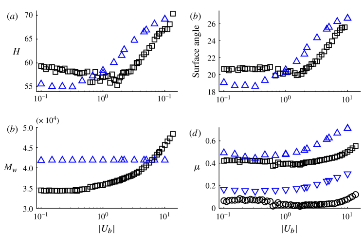
Figure 19: A summary of steady-state results for simulations in the narrow slot showing the dependence on $|U_{b}|$ of (a) depth at the blade, $x=0$, (b) the leading-order surface slope angle, (c) the mass of material in the wedge $M_{w}=\sum_{j}(u_{j}-U_{b})/|U_{b}|$, and (d) the effective horizontal and vertical friction coefficients, $(\mu_{x},\mu_{z})=(F_{x},F_{y})/(gM_{w})$, where $(F_{x},F_{z})$ is the net force on the blade ($F_{x}<F_{z}$). The squares and circles show the results with an underlying layer; the triangles show the results without one.

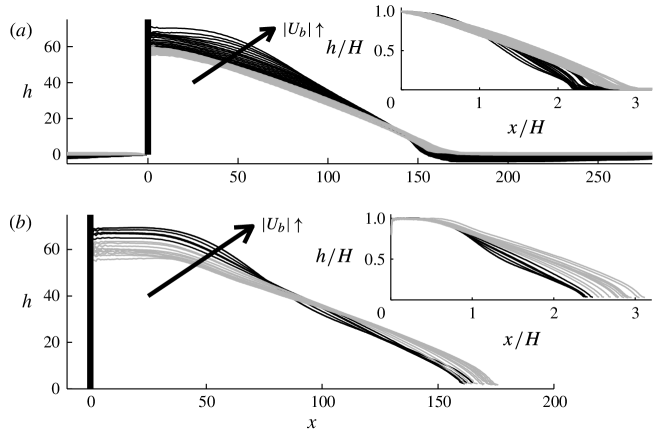
Figure 20: (a) Steady-state wedge profiles for simulations with varying bulldozer speed in the narrow slot (a) with and (b) without an underlying layer. The black lines denote the profiles for $|U_{b}|\geq 3.2$ (beyond the minimum of the curve in 19(a)); the grey lines denote the simulations with $|U_{b}|<3.0$. In the insets, the profiles are rescaled by the depth at the blade, $x=0$, to furnish the master curves, after subtracting the level of the incoming layer in (a).

4.3.2 Lateral spreading

The laterally spreading solution with an underlying plane for $|U_{b}|=1$ is displayed in figure 21. Because the bulldozing is planar in the simulation, the spreading is symmetrical, unlike in the experiments. Despite this difference, there are still qualitative similarities between the simulations and experiments. Further details of the simulation are shown in figure 22, which plots snapshots of the perpendicular profiles along the midsection of the dune (i.e. $y=0$) and its lateral profile along the blade (the depth at $x=0$) at different times. These profiles appear to be self-similar, as indicated by the insets of the figure, which scale the perpendicular profiles with $H(0,t)$ and the lateral profiles with $Y(t)$, the lateral extent of the dune. Figure 22 also shows the corresponding results for a simulation without an underlying layer. Qualitatively, the character of the evolution is very similar. In particular, for the simulation without an underlying layer, the self-similar lateral profile adopts a form that is well fitted by the parabolic similarity solution in (17). It should be noted that the perpendicular master profile shown in the inset of figure 22(a) is somewhat steeper at the blade than the narrow-slot simulations in figure 20a, and therefore compares more favourably with the experimental profiles.

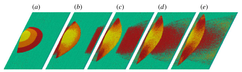
Figure 21: Particles positions at $t=0$, 100, 200, 300 and 400 for a lateral spreading simulation with an underlying layer and $|U_{b}|=1$. The particles are coloured according to their initial height. (Video of this simulation is available as supplementary material).

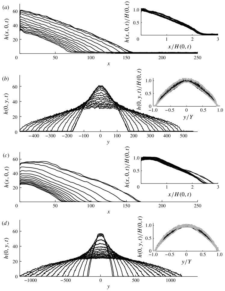
Figure 22: Lateral spreading simulations (a,b) with and (c,d) without an underlying layer. Shown are (a,c) the perpendicular $h(x,0,t)$, and (b,d) the lateral $H(y,t)=h(0,y,t)$ profiles. The insets show scaled versions of these profiles, with the perpendicular profiles in (a,c) scaled by depth at the blade, and the lateral profile in (b,d) scaled by the half-width $Y(t)$. The grey lines in the insets show the initial and final profiles. The times of the snapshots are given by $t=t_{min}+(t_{max}-t_{min})\left({j}/{15}\right)^{5/2}$, $j=0$, 1, $...$, 15, with $(t_{min},t_{max})=(0.1,2000)$ and $(0.5,11650)$ in (a,b) and (c,d), respectively.

Figure 23 plots the time series of $H(0,t)$, $Y(t)$ and the maximum perpendicular run-out, $X(0,t)$, for both simulations in figure 22. Also included are best-fit power-law fits to these series. For $H(0,t)$ and $X(0,t)$, the data are roughly fitted by $t^{-1/5}$, which is the self-similar scaling predicted by (18b) (the best-fit powers are $-0.22$ with the underlying layer and $-0.19$ without it). However, although the best-fit power law for $Y(t)$ is not too far from $t^{2/5}$ for the simulation without an underlying layer (the best-fit power is $0.34$), it is quite different with the basal layer (being $0.26$). The key to explaining this discrepancy is to examine the total mass contained in the dune $M_{w}$: for the simulation without the underlying layer, the best-fit powers for $H$, $Y$ and $X(0,t)$ sum closely to zero, confirming the notion that the dune is a slowly spreading, but constant-mass structure. With the underlying layer, however, the exponents do not sum to zero, suggesting that the dune is losing mass as time progresses. Indeed, direct measurements (figure 23a) indicate a power-law decay of $M_{w}$ beyond an initial transient, with a best-fit exponent of $-0.14$ which is close to the summed exponents of $H$, $Y$ and $X(0,t)$. The mass loss occurs because the backflow under the blade effectively skims off material from the underlying layer and further builds up the dune at the beginning of the simulation. Due to lateral spreading, however, the backflow weakens with time, returning mass to the underlying layer. Evidently, the scaling of $Y(t)$ is the main casualty, probably because the shallow edges of the dune are affected most.

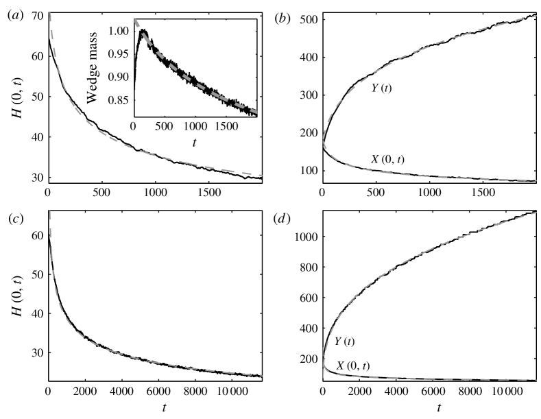
Figure 23: Time series of (a,c) maximum depth $H(0,t)$ and (b,d) half-width $Y(t)$ and perpendicular run-out $X(0,t)$, for the simulations shown in figure 22. The half-width $Y(t)$ and run-out $X(0,t)$ are determined by fitting a second order polynomial $p(x,y)$ to the surface profile and then finding the positions for which $p(0,Y)=p(X,0)=0$. The dashed grey lines are the best fits for the parameters $(Y_{0},X_{0},\mu,p_{1},p_{2})$ to the data for $t>50$, assuming $Y(t)=Y_{0}\,(1+t/t_{0})^{p_{1}}$, $X(0,t)=X_{0}\,(1+t/t_{0})^{p_{2}}$, $H(0,t)=\mu\,X(0,t)$ and $t_{0}={Y_{0}}^{2}/(5\,X_{0}\,|U_{b}|)$ as predicted by the theory. With the underlying layer (a,b), the best fit power for $H$, $X(0,t)$ is $-0.22$ and for $Y$ is $0.26$ for with a friction coefficient of 0.41; without that layer (c,d), the powers are $-0.19$, and $0.34$, with a friction coefficient of 0.41. In panel (a), the inset shows the mass of material in the wedge normalized by its initial value as a function of time; the grey dashed line shows the best power-law fit with an exponent $-0.14$.

5 Conclusion

In this paper, we have studied the granular flow created by bulldozing a pile of grains over a level surface, both experimentally and theoretically. In the experiments, we bulldozed a granular mound over a rotating table, demonstrating how an avalanching dune is driven forwards in two phases. A first rapid adjustment takes place perpendicular to the blade, with the emergence of a quasi-steady avalanching state characterized by a profile that has an almost constant slope. This rapid adjustment is followed by a second slower phase of lateral spreading parallel to the blade. We constructed two simple depth-averaged theoretical models to describe the perpendicular steady-state avalanching and lateral spreading. The first model captures the leading-order linear slope of the experimental dunes, but not the finer details of their nonlinear shape. The experimental observations of asymmetrical radial spreading and outward migration are matched qualitatively, but not quantitatively, by the second model.

Our theoretical discussion is further shored up by DEM simulations, which reproduce the phenomenology seen in the experiments and offer a better comparison with some of the more detailed observations. We have not, however, exploited the full power of the DEM simulations in dissecting the flow dynamics non-invasively, or to study the detailed effect of some of the physical parameters, such as the depth of the underlying layer and the detailed boundary conditions on the blade. Our computations do suggest that both of these are key in determining the shape of the perpendicular profile at the blade. As an alternative to DEM, two-dimensional computations of the free-surface flow are also feasible for fluid modelled with the empirically based model rheology of GDR Midi (2004). The comparison of such computations with our experiments and DEM simulations will probably act as a sensitive test of the empirical rheology.

From an experimental perspective, our approach has focused mainly on recording the shapes of the free surfaces of bulldozed dunes. Although it is difficult to determine the full velocity field within the dune non-invasively, it is certainly possible to measure the surface velocity profile. Indeed, by using a mixture of grains of different colours (in this case, black and white), we were able to take some preliminary particle image velocimetry measurements for dunes of aquarium sand, as shown in figure 24. The avalanching flow at the front of the dune is clear in these measurements, which provide a more demanding test of any theoretical model. The perpendicular surface velocity increases towards the front of the dune, as the avalanching particles accelerate. There is also a significant lateral surface velocity, which is probably due to the overall surface shape. The spatial structure of the flow field warrants further investigation.

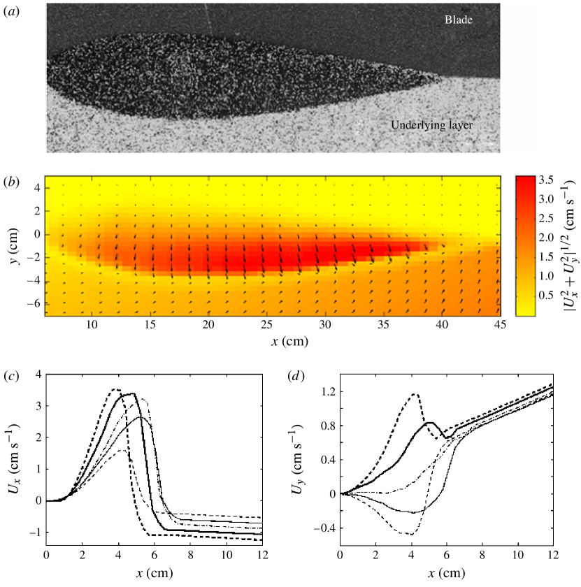
Figure 24: Surface velocity field of a dune of aquarium sand. (a) shows the raw image and (b) depicts the surface speed in cm/s as a density over the plane of the image. The surface velocity components perpendicular and parallel to the blade, $U_{x}$ and $U_{y}$, are plotted as arrows in (b), and then in (c,d) along the lateral positions $y=10$ cm (dashed), $15$ cm (continuous), $20$ cm (dashed-dotted), $25$ cm (thick continuous) and $30$ cm (thick dashed). Note that, in view of the inclination of the surface, the velocity field $(U_{x},U_{y})$ does not correspond to the horizontal Cartesian velocity $(u,v)$.

As a model granular flow, the two-dimensional bulldozer could be considered as midway in complexity between the inclined-plane or shear-cell configuration and more complicated flows like the rotating drum. The inclined-plane and shear-cell tests are steady uniform flows that are free of any yield surfaces or rigid plugs. The streamlines in the rotating drum, in contrast, piece together paths of acceleration and deceleration, with flow bounded from below by a yield surface. The wedges of our bulldozed flows do not appear to contain any yield surfaces, but particles do experience phases of acceleration and deceleration as they traverse the average streamlines. Thus, the flow might well prove useful as a probe of granular rheology, a stepping stone from the inclined plane or the shear cell to the rotating drum.

Of course, although the mean flow of a steady two-dimensional bulldozer possesses closed streamlines, the finite size of particles and their granular temperature allows particles to cross transport barriers and mix. Moreover, for our rotating bulldozer, the slower lateral spreading also implies transport. Indeed, qualitative experiments using aquarium sand of different colours highlighted the exchange of granular material between the initial dune and the underlying layer; as is apparent in figure 25. Such mixing is also clear in the DEM simulations (figure 21). Quantitative measurements and modelling of this phenomenon are beyond the scope of the present paper but may be of interest, for example, when on is considering the transport of pollutants over soil and the avoidance of contamination is a critical objective. A detailed exploration of particle migration would also be relevant to granular segregation; the bulldozer being an interesting experimental configuration in which to study this phenomenon.

Another interesting observation which we did not explore in detail was the effect of slip over the surface of the rotating table. When the table was not covered by sandpaper, but was left as a smoother wooden surface, the uniform layer initially emplaced clearly began to slide during the approach to the bulldozer. In particular, the flow divided up into three characteristic regions. Well ahead of the dune, the underlying layer remained flat and stationary, while closer to the blade, the dune built up into a quasi-static avalanching mound that appeared similar to those documented earlier. In between, the sliding underlying layer created a buffer zone with a much shallower slope than the dune behind it. Interestingly, the compression incurred over this buffer appeared to generate surface features reminiscent of a fine wrinkling pattern (cf. Alarcón et al., 2010).

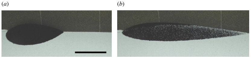
Figure 25: Photographs from an experiment with $m=1000$ g, $\Omega=0.05$ rad s^-1 and $y_{0}=25$ cm and different coloured aquarium sand. The initial pile of black sand was bulldozed over a layer of white sand. Panel (a) shows the collision of the dune with the blade. Relatively quickly, an exchange of particles between the sandpile and the underlying bed is visible, as shown in panel (b) (at $t=35$ s). Scale bar in (a) is $15$ cm.

References

- Alarcón et al. (2010) Alarcón, H., Ramos, O., Vanel, L., Vittoz, F., Melo, F. & Géminard, J. C. 2010 Softening induced instability of a stretched cohesive granular layer. Phys. Rev. Lett. 105, 208001.
- Andreotti (2012) Andreotti, B. 2012 Sonic sands. Rep. Prog. Phys. 75, 026602.
- Andreotti et al. (2013) Andreotti, B., Forterre, Y. & Pouliquen, O. 2013 Granular Media: Between Fluid and Solid. Cambridge University Press.
- Bagnold (1966) Bagnold, R. A. 1966 The shearing and dilatation of dry sand and the singing mechanism. Proc. Roy. Soc. A 295, 219–232.
- Balmforth & Kerswell (2005) Balmforth, N. J. & Kerswell, R. R. 2005 Granular collapse in two dimensions. J. Fluid Mech. 538(1), 399–428.
- Bitbol et al. (2009) Bitbol, A.-F., Taberlet, N., Morris, S. W. & McElwaine, J. N. 2009 Scaling and dynamics of washboard roads. Phys. Rev. E 79, 061308.
- Börzsönyi et al. (2009) Börzsönyi, T., Ecke, R. E. & McElwaine, J. N. 2009 Patterns in flowing sand: understanding the physics of granular flow. Phys. Rev. Lett. 103, 178302.
- Börzsönyi et al. (2008) Börzsönyi, T., Halsey, T. C. & Ecke, R. E. 2008 Avalanche dynamics on a rough inclined plane. Phys. Rev. E 78(1), 011306.
- Cundall & Strack (1979) Cundall, P. A. & Strack, O. D. 1979 A discrete numerical model for granular assemblies. Geotechnique 29, 47–65.
- Ding et al. (2011) Ding, Y., Gravish, N. & Goldman, D. I. 2011 Drag induced lift in granular media. Phys. Rev. Lett. 106(2), 028001.
- Douady et al. (2006) Douady, S., Manning, A., Hersen, P., Elbelrhiti, H., Protiere, S., Daerr, A. & Kabbachi, B. 2006 The song of the dunes as a self-synchronized instrument. Phys. Rev. Lett. 97, 018002.
- Forterre & Pouliquen (2008) Forterre, Y. & Pouliquen, O. 2008 Flows of dense granular media. Annu. Rev. Fluid Mech. 40, 1–24.
- GDR Midi (2004) GDR Midi, . 2004 On dense granular flows. Eur. Phys. J. E. 14, 341–365.
- Geng & Behringer (2005) Geng, J. & Behringer, R. P. 2005 Slow drag in two-dimensional granular media. Phys. Rev. E 71(1), 011302.
- Gravish et al. (2010) Gravish, N., Umbanhowar, P. B. & Goldman, D. I. 2010 Force and flow transition in plowed granular media. Phys. Rev. Lett. 105(12), 128301.
- Guillard et al. (2013) Guillard, F., Forterre, Y. & Pouliquen, O. 2013 Depth-independent drag force induced by stirring in granular media. Phys. Rev. Lett. 110(13), 138303.
- Guo et al. (2012) Guo, H., Goldsmith, J., Delacruz, I., Tao, M., Luo, Y. & Koehler, S. A. 2012 Semi-infinite plates dragged through granular beds. J. Stat. Mech. Theor. Exp. 7, P07013.
- Hewitt et al. (2012) Hewitt, I. J., Balmforth, N. J. & McElwaine, J. N. 2012 Granular and fluid washboards. J. Fluid Mech. 692, 446–463.
- Holyoake & McElwaine (2012) Holyoake, Alex J. & McElwaine, Jim N. 2012 High-speed granular chute flows. J. Fluid Mech. 710, 35–71.
- Jaeger et al. (1996) Jaeger, H. M., Nagel, S. R. & Behringer, R. P. 1996 Granular solids, liquids, and gases. Rev. Mod. Phys. 68(4), 1259–1273.
- Jop et al. (2006) Jop, P., Forterre, Y. & Pouliquen, O. 2006 A constitutive law for dense granular flows. Nature 441, 727–730.
- Lacaze & Kerswell (2009) Lacaze, L. & Kerswell, R.R. 2009 Axisymmetric granular collapse: a transient three dimensional flow test of viscoplasticity. Phys. Rev. Lett. 102, 108305.
- Lagrée et al. (2011) Lagrée, P.-Y., Staron, L. & Popinet, S. 2011 The granular column collapse as a continuum: validity of a two-dimensional navier-stokes model with a -rheology. J. Fluid Mech. 686, 378–408.
- Lajeunesse et al. (2004) Lajeunesse, E., Mangeney-Castelnau, A. & Vilotte, J. P. 2004 Spreading of a granular mass on a horizontal plane. Phys. Fluids 16, 2371.
- Mather (1963) Mather, K. B. 1963 Why do roads corrugate? Sci. Am. 208, 128–136.
- Percier et al. (2011) Percier, B., Manneville, S., McElwaine, J. N., Morris, S. W. & Taberlet, N. 2011 Lift and drag forces on an inclined plow moving over a granular surface. Phys. Rev. E 84, 051302.
- Percier et al. (2013) Percier, B., Manneville, S. & Taberlet, N. 2013 Modeling a washboard road: From experimental measurements to linear stability analysis. Phys. Rev. E 87, 012203.
- Pouliquen (1999a) Pouliquen, O. 1999a On the shape of granular fronts down rough inclined planes. Phys. Fluids 11, 1956–1958.
- Pouliquen (1999b) Pouliquen, O. 1999b Scaling laws in granular flows down rough inclined planes. Phys. Fluids 11, 542–548.
- Sauret (2012) Sauret, A. 2012 Smoothing out sandpiles: rotational bulldozing of granular material. W. H. O. I. Tech. Report 53.
- Savage & Hutter (1991) Savage, S.B. & Hutter, K. 1991 The dynamics of avalanches of granular materials from initiation to runout. part i: analysis. Acta Mechanica 86, 201–223.
- Taberlet et al. (2007) Taberlet, N., Morris, S. W. & McElwaine, J. N. 2007 Washboard road: The dynamics of granular ripples formed by rolling wheels. Phys. Rev. Lett. 99, 068003.
- Taberlet et al. (2006) Taberlet, N., Richard, P. & Hinch, J.E. 2006 S shape of a granular pile in a rotating drum. Phys. Rev. E 73, 050301.