Finite-strain formulation and FE implementation of a constitutive model for powder compaction

Abstract

A finite-strain formulation is developed, implemented and tested for a constitutive model capable of describing the transition from granular to fully dense state during cold forming of ceramic powder. This constitutive model (as well as many others employed for geomaterials) embodies a number of features, such as pressure-sensitive yielding, complex hardening rules and elastoplastic coupling, posing considerable problems in a finite-strain formulation and numerical implementation. A number of strategies are proposed to overcome the related problems, in particular, a neo-Hookean type of modification to the elastic potential and the adoption of the second Piola-Kirchhoff stress referred to the intermediate configuration to describe yielding. An incremental scheme compatible with the formulation for elastoplastic coupling at finite strain is also developed, and the corresponding constitutive update problem is solved by applying a return mapping algorithm.

Keywords: plasticity; elastoplastic coupling; finite element method; automatic differentiation

1 Introduction

The formulation and implementation of elastoplastic constitutive equations for metals at large strain have been thoroughly analyzed in the last thirty years, see for instance [1, 2], so that nowadays they follow accepted strategies. For these materials, pressure-insensitive yielding, $J_{3}$-independence, and incompressibility of plastic flow strongly simplify the mechanical behaviour, while frictional-cohesive and rock-like materials (such as granular media, soils, concretes, rocks, ceramics and powders) are characterized by pressure-sensitive, $J_{3}$-dependent yielding, dilatant/contractant flow, nonlinear elastic behaviour even at small strain and elastoplastic coupling. There have been several attempts to generalize treatment of metal plasticity at large strain in this context [3, 4, 5, 6, 7, 8, 9], but many problems still remain not completely solved. These include the form of the elastic potential, the stress measure to be employed in the yield function, which has to provide an easy interpretation of experiments, the flow rule and the elastic-plastic coupling laws.

The main difficulty in the practical application of finite-strain elastoplasticity models, as opposed to their small-strain counterparts, is related to development and implementation of incremental (i.e., finite-step) constitutive relationships. The difficulties lie, for instance, in formulation and solution of the highly nonlinear constitutive update problem, consistent treatment of plastic incompressibility (or plastic volume changes), and consistent linearization of the incremental relationships. The last issue is of the utmost importance for overall computational efficiency of the finite element models because consistent linearization (consistent tangent) is needed to achieve the quadratic convergence of the Newton method.

In the present paper, the model for cold forming of ceramic powders proposed by Piccolroaz et al. [10, 11] (called ‘PBG model’ in the following) is developed for large strain analyses, implemented in the finite element method and numerically tested. The need for this large-strain generalization is related to the fact that during ceramic forming the mean strain can easily reach 50%, while peaks can touch 80%. The differences between a small strain and a large strain analysis can be appreciated from Fig. 1, where small-strain and large-strain predictions are reported for the force/displacement relation at the top of a rigid mould containing an alumina ceramic powder. Results (taken from [12] and pertaining to a flat punch and to a punch with a ‘cross-shaped’ groove, respectively reported in Fig. 1a and 1b) clearly show that the large-strain analyses are more consistent and in closer agreement with experimental results than the analyses performed under the small strain hypothesis.

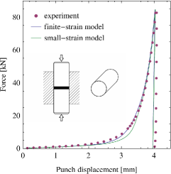
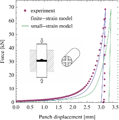
      (a)       (b)

Figure 1: Predictions of the small- and finite-strain versions of the PBG model for compression of alumina powder by: (a) flat punch (uniform uniaxial strain), (b) cross-shaped punch (nonuniform 3D deformation). The results are taken from [12].

The model for powder compaction can be considered as paradigmatic of the difficulties that can be encountered in the implementation of models for geomaterials, since many ‘unconventional’ features of plasticity are simultaneously present to describe the complex transition from a loose granular material (the powder) to a fully dense ceramic (the green body). These difficulties enclose: (i.) the pressure-sensitive, $J_{3}$-dependent yield function introduced by Bigoni and Piccolroaz [13] (‘BP yield function’ in the following), which is defined $+\infty$ in some regions outside the elastic domain; (ii.) a nonlinear elastic behaviour even at small strain, (iii.) changes in elastic response coupled to plastic deformation (elastoplastic coupling).

In this work, incremental (finite-step) constitutive equations are developed and implemented for the finite-deformation version of the PBG model. In order to improve the computational efficiency, the original model [11] is slightly modified, but its essential features, including the elastoplastic coupling, are preserved. Note that a consistent finite-element implementation of the elastoplastic coupling at finite strain has not been reported in the literature so far. The model is applied to simulate ceramic powder compaction with account for frictional contact interaction.

The above-mentioned implementation difficulties are efficiently handled by using an advanced hybrid symbolic-numeric approach implemented in AceGen, a symbolic code generation system [14, 15]. AceGen combines symbolic and algebraic capabilities of Mathematica, automatic differentiation (AD) technique, simultaneous optimization of expressions and automatic generation of computer codes, and it is an efficient tool for rapid prototyping of numerical procedures as well as for generation of highly optimized compiled codes (such as finite element subroutines). Finite element computations have been carried out using AceFEM, a highly flexible finite element code that is closely integrated with AceGen.

Selected results of 2D and 3D simulations of powder compaction processes have already been reported in [12], and the model predictions have been compared to experimental data showing satisfactory agreement, see for instance Fig. 1. However, the finite-strain formulation and the numerical strategies adopted for its implementation have not been presented in [12], as that paper was aimed at providing an overview of elastoplastic coupling in powder compaction processes. In the present paper, we provide the details of the formulation and implementation, and, as an application, we study the effect of friction and initial aspect ratio on compaction of alumina powder in a cylindrical die.

2 PBG model at small strain

The small-strain PBG model [10] is briefly described below as a reference for its finite-strain version introduced in the next section, with a slight modification to the notation to make it more convenient for the subsequent extension to the finite-strain framework. The model is fully defined by specifying the free energy, the yield condition, and the plastic flow rule, and these are provided below. For the details, including justification of the specific constitutive assumptions and calibration of the model for alumina powder, refer to Piccolroaz et al. [10].

2.1 Free energy

The total strain $\boldsymbol{\varepsilon}$ is decomposed into the elastic $\boldsymbol{\varepsilon}_{e}$ and plastic $\boldsymbol{\varepsilon}_{p}$ parts,

$$\boldsymbol{\varepsilon}=\boldsymbol{\varepsilon}_{e}+\boldsymbol{\varepsilon}_{p},$$ (1)

and the free energy is assumed in the following form,

$$\phi(\boldsymbol{\varepsilon},\boldsymbol{\varepsilon}_{p},p_{c})=c\,\operatorname{tr}\boldsymbol{\varepsilon}_{e}+(p_{0}+c)\left[\left(d-\frac{1}{d}\right)\frac{(\operatorname{tr}\boldsymbol{\varepsilon}_{e})^{2}}{2\tilde{\kappa}}+d^{1/n}\tilde{\kappa}\exp\left(-\frac{\operatorname{tr}\boldsymbol{\varepsilon}_{e}}{d^{1/n}\tilde{\kappa}}\right)\right]+\mu\operatorname{tr}\boldsymbol{\varepsilon}_{e}^{2}-\frac{\mu}{3}(\operatorname{tr}\boldsymbol{\varepsilon}_{e})^{2},$$ (2)

where the plastic strain $\boldsymbol{\varepsilon}_{p}$ and the forming pressure $p_{c}$ are adopted as internal variables, and $\boldsymbol{\varepsilon}_{e}=\boldsymbol{\varepsilon}-\boldsymbol{\varepsilon}_{p}$. The elastoplastic coupling is here introduced through the dependence of cohesion $c$, parameter $d$ and shear modulus $\mu$ on the forming pressure $p_{c}$, namely

$$c=c_{\infty}[1-\exp(-\Gamma\langle p_{c}-p_{cb}\rangle)],$$ (3)

$$d=1+B\langle p_{c}-p_{cb}\rangle,$$ (4)

$$\mu=\mu_{0}+c\left(d-\frac{1}{d}\right)\mu_{1},$$ (5)

where $\langle\cdot\rangle$ denotes the Macauley brackets operator, $\tilde{\kappa}=\kappa/(1+e_{0})$ and $\kappa$, $e_{0}$, $p_{0}$, $n$, $c_{\infty}$, $\Gamma$, $p_{cb}$, $B$, $\mu_{0}$ and $\mu_{1}$ are material parameters. Note that the elastoplastic coupling is related to the variation in $d$, so that, if $d$ remains constant and equal to one, the elastic properties of the material remain unchanged during plastic flow.

The forming pressure $p_{c}$ is assumed to depend on the volumetric part of the plastic strain through the following relationship

$$\operatorname{tr}\boldsymbol{\varepsilon}_{p}={\cal H}(p_{c}),\qquad{\cal H}(p_{c})=-\tilde{a}_{1}\exp\left(-\frac{\Lambda_{1}}{p_{c}}\right)-\tilde{a}_{2}\exp\left(-\frac{\Lambda_{2}}{p_{c}}\right),$$ (6)

where $\tilde{a}_{i}$ and $\Lambda_{i}$ are material parameters. In view of the above dependence, the free energy could formally be expressed solely in terms of the total strain $\boldsymbol{\varepsilon}$ and the plastic strain $\boldsymbol{\varepsilon}_{p}$. However, the dependence of $p_{c}$ on $\boldsymbol{\varepsilon}_{p}$ is implicit, i.e., $p_{c}$ cannot be expressed as an explicit function of $\boldsymbol{\varepsilon}_{p}$. It is thus convenient to keep $p_{c}$ as an internal variable with the additional constraint introduced by Eq. (6), see Section 4.3.

Note that the forming pressure $p_{c}$ and the cohesion $c$ are also used to define the yield surface (see below). The corresponding governing equations (6) and (3) are thus called ‘hardening laws’ in [10].

2.2 Inelastic strain rate

The elastoplastic coupling, introduced above through the dependence of the free energy $\phi$ on the plastic strain $\boldsymbol{\varepsilon}_{p}$ and the forming pressure $p_{c}$, is a crucial feature of the model. As a result, the stress depends not only on the elastic strain, but also on the internal variables. Indeed, the stress $\boldsymbol{\sigma}$ is defined by

$$\boldsymbol{\sigma}=\frac{\partial\phi}{\partial\boldsymbol{\varepsilon}},$$ (7)

and its rate involves the contributions due to the evolution of the internal variables,

$$\dot{\boldsymbol{\sigma}}=\frac{\partial\boldsymbol{\sigma}}{\partial\boldsymbol{\varepsilon}}[\dot{\boldsymbol{\varepsilon}}]+\frac{\partial\boldsymbol{\sigma}}{\partial\boldsymbol{\varepsilon}_{p}}[\dot{\boldsymbol{\varepsilon}}_{p}]+\frac{\partial\boldsymbol{\sigma}}{\partial p_{c}}\dot{p}_{c}=\mathbbm{E}[\dot{\boldsymbol{\varepsilon}}]+\mathbbm{P}[\dot{\boldsymbol{\varepsilon}}_{p}]+\textbf{\em P}\dot{p}_{c}=\mathbbm{E}[\dot{\boldsymbol{\varepsilon}}-\dot{\boldsymbol{\varepsilon}}_{\it in}].$$ (8)

Here, $\mathbbm{E}$ is the elastic fourth-order tensor, $\mathbbm{P}$ and P describe the elastoplastic coupling, and the inelastic strain rate $\dot{\boldsymbol{\varepsilon}}_{\it in}$ is defined as

$$\dot{\boldsymbol{\varepsilon}}_{\it in}=-\mathbbm{E}^{-1}\mathbbm{P}[\dot{\boldsymbol{\varepsilon}}_{p}]-\mathbbm{E}^{-1}[\textbf{\em P}\dot{p}_{c}].$$ (9)

The inelastic strain rate $\dot{\boldsymbol{\varepsilon}}_{\it in}$ is thus not equal to the plastic strain rate $\dot{\boldsymbol{\varepsilon}}_{p}$, and the former will be used in the plastic flow rule, which is crucial for a consistent treatment of the elastoplastic coupling, see Bigoni [16]. The model is rate-independent, hence by the time we understand here a time-like load parameter.

2.3 Yield condition

The yield condition is defined using the Bigoni–Piccolroaz (BP) yield function [13]

$$F(\boldsymbol{\sigma},p_{c})=f(p,p_{c})+\frac{q}{g(\theta)}\leq 0,$$ (10)

where

$$f(p,p_{c})=\left\{\begin{array}[]{ll}-Mp_{c}\sqrt{(\Phi-\Phi^{m})[2(1-\alpha)\Phi+\alpha]}&\mbox{if}\;\Phi\in[0,1],\\ +\infty&\mbox{otherwise},\end{array}\right.\quad\Phi=\frac{p+c}{p_{c}+c},$$ (11)

$$g(\theta)=\frac{1}{\cos[\beta\pi/6-(1/3)\cos^{-1}(\gamma\cos 3\theta)]},$$ (12)

and $p$, $q$ and $\theta$ are the usual invariants of the stress tensor,

$$p=-\frac{1}{3}\operatorname{tr}\boldsymbol{\sigma},\qquad q=\sqrt{3J_{2}},\qquad\theta=\frac{1}{3}\cos^{-1}\left(\frac{3\sqrt{3}}{2}\,\frac{J_{3}}{J_{2}^{3/2}}\right),$$ (13)

$$J_{2}=\frac{1}{2}\operatorname{tr}(\operatorname{dev}\boldsymbol{\sigma})^{2},\qquad J_{3}=\frac{1}{3}\operatorname{tr}(\operatorname{dev}\boldsymbol{\sigma})^{3},\qquad\operatorname{dev}\boldsymbol{\sigma}=\boldsymbol{\sigma}-\frac{1}{3}(\operatorname{tr}\boldsymbol{\sigma})\textbf{\em I}.$$ (14)

The forming pressure $p_{c}$ and the cohesion $c$, which depends on $p_{c}$ through Eq. (3), define the size of the yield surface $F=0$ and its position along the hydrostatic axis. Parameters $M$, $m$, $\alpha$, $\beta$ and $\gamma$ define the shape of the yield surface and are assumed constant.

It is seen from Eq. (11) that the BP yield function $F$ is defined infinity for $p\not\in[-c,p_{c}]$, so it cannot be evaluated numerically for an arbitrary stress state, and incremental schemes employing, for instance, the return mapping algorithm cannot be applied directly. Therefore, following Stupkiewicz et al. [17], an alternative implicit yield function $F^{\ast}$ is used in practice, which has the same zero level set $F^{\ast}=0$ as the original yield function (i.e., $F=0$) but behaves well for arbitrary stress states, see Section 4.1.

2.4 Plastic flow rule

The flow rule is expressed in terms of the inelastic strain rate $\dot{\boldsymbol{\varepsilon}}_{\it in}$ rather than the plastic strain rate $\dot{\boldsymbol{\varepsilon}}_{p}$, see Bigoni [16],

$$\dot{\boldsymbol{\varepsilon}}_{\it in}=\dot{\lambda}\hat{\textbf{\em n}},\qquad\hat{\textbf{\em n}}=\textbf{\em n}-\frac{1}{3}\,\epsilon(1-\Phi)(\operatorname{tr}\textbf{\em n})\textbf{\em I},\qquad\textbf{\em n}=\frac{\partial F}{\partial\boldsymbol{\sigma}},$$ (15)

where $\dot{\lambda}$ is the plastic multiplier satisfying the usual complementarity conditions,

$$\dot{\lambda}\geq 0,\qquad F\leq 0,\qquad\dot{\lambda}F=0.$$ (16)

Here, $\epsilon$ is a parameter that governs non-associativity of the flow rule ($0\leq\epsilon<1$), and $\epsilon=0$ corresponds to the associated flow rule.

3 PBG model at finite strain

The PBG model [10] has been extended to the finite-strain framework by the same group of authors in [11]. In that model, the usual multiplicative decomposition of the deformation gradient has been adopted, the free energy has been expressed in terms of the logarithmic elastic strain while keeping the same form (2) of the free energy function, and the BP yield condition has been expressed in terms of the Biot stress tensor referred to the initial configuration. With regard to the elastoplastic coupling and plastic flow rule, the Biot stress and its conjugate strain measure have been used to define the inelastic strain rate (using the general framework developed by Bigoni [16]), and that inelastic strain rate has subsequently been used in the plastic flow rule. Finally, a complete set of rate equations has been derived; however, incremental formulation and it finite element implementation have not been attempted.

In this section, a finite-strain formulation of the PBG model is introduced, which is more convenient for the finite-element implementation than the formulation of Piccolroaz et al. [11]. At the same time, the essential features of that model are preserved, namely the specific form of the free energy function, the elastoplastic coupling framework of Bigoni [16], the BP yield condition [13], and the plastic flow rule. The main difference is in the selection of the internal variables and in the choice of the stress and strain measures used to define the inelastic strain rate and to formulate the flow rule. Also, the yield condition is here expressed in terms of the second Piola-Kirchhoff stress referred to the intermediate configuration rather than in terms of the Biot stress referred to the initial reference configuration which seems more consistent with respect to the experimental testing procedures that are typically used to calibrate the model.

3.1 Free energy

The deformation gradient F is multiplicatively split into elastic $\textbf{\em F}_{e}$ and plastic $\textbf{\em F}_{p}$ parts,

$$\textbf{\em F}=\textbf{\em F}_{e}\textbf{\em F}_{p},$$ (17)

and the following standard kinematic quantities are introduced,

$$\textbf{\em C}=\textbf{\em F}^{T}\textbf{\em F},\qquad\textbf{\em C}_{p}=\textbf{\em F}_{p}^{T}\textbf{\em F}_{p},\qquad\textbf{\em b}_{e}=\textbf{\em F}_{e}\textbf{\em F}_{e}^{T}=\textbf{\em F}\textbf{\em C}_{p}^{-1}\textbf{\em F}^{T},$$ (18)

respectively, the total and plastic right Cauchy–Green tensors, and the elastic left Cauchy–Green tensor. Furthermore, we have

$$J=J_{e}J_{p},\quad J=\det\textbf{\em F},\quad J_{e}=\det\textbf{\em F}_{e}=(\det\textbf{\em b}_{e})^{1/2},\quad J_{p}=\det\textbf{\em F}_{p}=(\det\textbf{\em C}_{p})^{1/2}.$$ (19)

In order to conveniently treat the volumetric strains, which are essential in modeling of powder compaction, the logarithmic elastic and plastic strain tensors are introduced,

$$\boldsymbol{\epsilon}_{e}=\log\textbf{\em V}_{e}=\frac{1}{2}\log\textbf{\em b}_{e},\qquad\textbf{\em E}_{p}^{(0)}=\log\textbf{\em U}_{p}=\frac{1}{2}\log\textbf{\em C}_{p},$$ (20)

where $\textbf{\em F}_{e}=\textbf{\em V}_{e}\textbf{\em R}_{e}$, $\textbf{\em b}_{e}=\textbf{\em V}_{e}^{2}$, $\textbf{\em F}_{p}=\textbf{\em R}_{p}\textbf{\em U}_{p}$, and $\textbf{\em C}_{p}=\textbf{\em U}_{p}^{2}$. The well-known benefit of using the logarithmic strain measure is that the volumetric strain is simply obtained as a trace of the corresponding strain tensor, and the total volumetric strain is additively decomposed into elastic and plastic contributions.

Following Piccolroaz et al. [11], the free energy can be assumed in the same functional form as in the small-strain model, Eq. (2), with the infinitesimal elastic strain $\boldsymbol{\varepsilon}_{e}$ simply replaced by the logarithmic strain $\boldsymbol{\epsilon}_{e}$. However, this form is not efficient in numerical implementation, and a modified free energy function is adopted in this work. For completeness, application of the original free energy of Piccolroaz et al. [11] is discussed in Appendix A.

In the modified free energy function, the volumetric behavior is described in terms of the logarithmic elastic strain $\boldsymbol{\epsilon}_{e}$, just like in the original model [11], while the shear behavior is described by the term of the neo-Hookean type formulated for the isochoric part of the elastic left Cauchy–Green tensor $\textbf{\em b}_{e}$, namely

$$\phi(\textbf{\em C},\textbf{\em C}_{p},p_{c})=c\,\operatorname{tr}\boldsymbol{\epsilon}_{e}+(p_{0}+c)\left[\left(d-\frac{1}{d}\right)\frac{(\operatorname{tr}\boldsymbol{\epsilon}_{e})^{2}}{2\tilde{\kappa}}+d^{1/n}\tilde{\kappa}\exp\left(-\frac{\operatorname{tr}\boldsymbol{\epsilon}_{e}}{d^{1/n}\tilde{\kappa}}\right)\right]+\frac{1}{2}\mu(\bar{I}_{2}-3),$$ (21)

where

$$\bar{I}_{2}=\operatorname{tr}\bar{\textbf{\em b}}_{e}=J_{e}^{-2/3}\operatorname{tr}\textbf{\em b}_{e},\qquad\det\bar{\textbf{\em b}}_{e}=1.$$ (22)

The right Cauchy–Green tensor C is adopted as a relevant measure of the total strain in view of the standard objectivity argument, and the plastic right Cauchy–Green tensor $\textbf{\em C}_{p}$ is adopted as an internal variable. Since elastic strains are here relatively small, the present modification of the free energy function with respect to that of [11] does not noticeably affect the actual elastic response.

The free energy (21) involves two invariants characterizing the elastic strain, $\operatorname{tr}\boldsymbol{\epsilon}_{e}$ and $\bar{I}_{2}$, that can be easily expressed in terms of C and $\textbf{\em C}_{p}$. Indeed, in view of (18) and (20), we have

$$J_{e}^{2}=(\det\textbf{\em C})(\det\textbf{\em C}_{p}^{-1}),\qquad\operatorname{tr}\textbf{\em b}_{e}=\operatorname{tr}(\textbf{\em C}\textbf{\em C}_{p}^{-1}),$$ (23)

so that

$$\operatorname{tr}\boldsymbol{\epsilon}_{e}=\frac{1}{2}\log J_{e}^{2},\qquad\bar{I}_{2}=(J_{e}^{2})^{-1/3}\operatorname{tr}(\textbf{\em C}\textbf{\em C}_{p}^{-1}).$$ (24)

Parameters $c$, $d$ and $\mu$ in the free energy (21) are assumed to depend on the forming pressure $p_{c}$ through Eqs. (3)–(5), exactly as in the small-strain model, while the forming pressure $p_{c}$ is related to $\textbf{\em C}_{p}$ by

$$(\det\textbf{\em C}_{p})^{1/2}-1={\cal H}(p_{c}).$$ (25)

The above relationship is a consistent generalization of Eq. (6)₁ to the finite deformation regime, where function ${\cal H}(p_{c})$ is specified by Eq. (6)₂.

3.2 Inelastic strain rate

The inelastic strain rate and subsequently the flow rule are introduced using the Green strain tensor $\textbf{\em E}^{(2)}=\frac{1}{2}(\textbf{\em C}-\textbf{\em I})$ and its conjugate stress tensor, the second Piola–Kirchhoff stress $\textbf{\em T}^{(2)}$. This is a particularly convenient choice because the second Piola–Kirchhoff stress $\textbf{\em T}^{(2)}$ is directly obtained as the derivative of the free energy with respect to C using the following standard relationship:

$$\textbf{\em T}^{(2)}=\frac{\partial\phi}{\partial\textbf{\em E}^{(2)}}=2\frac{\partial\phi}{\partial\textbf{\em C}}.$$ (26)

Clearly, the material response is invariant with respect to the choice of a pair of conjugate strain and stress measures, see [18, 16]. Evaluation of the rate of $\textbf{\em T}^{(2)}$ defines the inelastic strain rate $\dot{\textbf{\em E}}_{\it in}$ according to

$$\dot{\textbf{\em T}}{}^{(2)}=\frac{\partial\textbf{\em T}^{(2)}}{\partial\textbf{\em E}^{(2)}}[\dot{\textbf{\em E}}{}^{(2)}]+\frac{\partial\textbf{\em T}^{(2)}}{\partial\textbf{\em C}_{p}}[\dot{\textbf{\em C}}_{p}]+\frac{\partial\textbf{\em T}^{(2)}}{\partial p_{c}}\dot{p}_{c}=\mathbbm{E}[\dot{\textbf{\em E}}{}^{(2)}]+\mathbbm{P}[\dot{\textbf{\em C}}_{p}]+\textbf{\em P}\dot{p}_{c}=\mathbbm{E}[\dot{\textbf{\em E}}{}^{(2)}-\dot{\textbf{\em E}}_{\it in}],$$ (27)

where $\mathbbm{E}=\partial\textbf{\em T}^{(2)}/\partial\textbf{\em E}^{(2)}=2\partial\textbf{\em T}^{(2)}/\partial\textbf{\em C}$, $\mathbbm{P}=\partial\textbf{\em T}^{(2)}/\partial\textbf{\em C}_{p}$, $\textbf{\em P}=\partial\textbf{\em T}^{(2)}/\partial p_{c}$, and

$$\dot{\textbf{\em E}}_{\it in}=-\mathbbm{E}^{-1}\mathbbm{P}[\dot{\textbf{\em C}}_{p}]-\mathbbm{E}^{-1}[\textbf{\em P}\dot{p}_{c}].$$ (28)

3.3 Yield condition

The yield condition is assumed to be defined by the BP yield function (10) expressed in terms of the second Piola-Kirchhoff stress $\textbf{\em T}^{(2)}_{e}$ referred to the intermediate configuration,

$$\textbf{\em T}^{(2)}_{e}=J_{e}\textbf{\em F}_{e}^{-1}\boldsymbol{\sigma}\textbf{\em F}_{e}^{-T}=J_{p}^{-1}\textbf{\em F}_{p}\textbf{\em T}^{(2)}\textbf{\em F}_{p}^{T},$$ (29)

where $\boldsymbol{\sigma}=J^{-1}\textbf{\em F}\textbf{\em T}^{(2)}\textbf{\em F}^{T}$ is the Cauchy stress, so that we have

$$F(\textbf{\em T}^{(2)}_{e},p_{c})\leq 0,$$ (30)

and the yield function $F$ is now defined by Eq. (10) through the invariants of $\textbf{\em T}^{(2)}_{e}$,

$$p=-\frac{1}{3}\operatorname{tr}\textbf{\em T}^{(2)}_{e},\qquad J_{2}=\frac{1}{2}\operatorname{tr}(\operatorname{dev}\textbf{\em T}^{(2)}_{e})^{2},\qquad J_{3}=\frac{1}{3}\operatorname{tr}(\operatorname{dev}\textbf{\em T}^{(2)}_{e})^{3}.$$ (31)

The above invariants, and thus the yield function, can be explicitly expressed in terms of the second Piola-Kirchhoff stress $\textbf{\em T}^{(2)}$ and the plastic right Cauchy–Green tensor $\textbf{\em C}_{p}$, the latter playing the role of a hardening variable. Indeed, we have

$$p=-\frac{1}{3}J_{p}^{-1}\operatorname{tr}(\textbf{\em T}^{(2)}\textbf{\em C}_{p}),\quad J_{2}=\frac{1}{2}J_{p}^{-2}\operatorname{tr}[\operatorname{dev}(\textbf{\em T}^{(2)}\textbf{\em C}_{p})]^{2},\quad J_{3}=\frac{1}{3}J_{p}^{-3}\operatorname{tr}[\operatorname{dev}(\textbf{\em T}^{(2)}\textbf{\em C}_{p})]^{3},$$ (32)

which is easily verified in view of the following identity holding for $n=1,2,\ldots$,

$$\operatorname{tr}(\textbf{\em T}^{(2)}_{e})^{n}=J_{p}^{-n}\operatorname{tr}(\textbf{\em T}^{(2)}\textbf{\em C}_{p})^{n},$$ (33)

and a similar identity holding for the respective deviators.

Note that the yield function was expressed in [11] in terms of the Biot stress tensor referred to the initial configuration. The present choice of $\textbf{\em T}^{(2)}_{e}$ is motivated by the typical model calibration procedures which are based on the Cauchy stress or the nominal stress referred to the intermediate configuration, see, for instance, [4]. Considering that the elastic strains are relatively small, the stress tensor $\textbf{\em T}^{(2)}_{e}$ is, in a sense ‘close’ to the Cauchy stress tensor $\boldsymbol{\sigma}$, hence provides a physically sound description of the yield surface. At the same time, as shown above, the yield function depending on $\textbf{\em T}^{(2)}_{e}$ can be equivalently expressed solely in terms of $\textbf{\em T}^{(2)}$ and $\textbf{\em C}_{p}$ which is not possible if the Cauchy stress is used instead.

3.4 Plastic flow rule

The flow rule is expressed in terms of the inelastic strain rate $\dot{\textbf{\em E}}_{\it in}$ defined in Eq. (28) and the plastic flow direction tensor $\hat{\textbf{\em N}}$ corresponding to the second Piola–Kirchhoff stress $\textbf{\em T}^{(2)}$. The finite-strain counterpart of the flow rule (15) is thus the following,

$$\dot{\textbf{\em E}}_{\it in}=\dot{\lambda}\hat{\textbf{\em N}},\qquad\hat{\textbf{\em N}}=\textbf{\em N}-\frac{1}{3}\,\epsilon(1-\Phi)\operatorname{tr}(\textbf{\em N}\textbf{\em C}_{p}^{-1})\textbf{\em C}_{p},\qquad\textbf{\em N}=\frac{\partial F}{\partial\textbf{\em T}^{(2)}},$$ (34)

with the usual complementarity conditions (16). The term $\operatorname{tr}(\textbf{\em N}\textbf{\em C}_{p}^{-1})\textbf{\em C}_{p}$ in the formula for $\hat{\textbf{\em N}}$ corresponds to the volumetric part $(\operatorname{tr}\textbf{\em N}_{e})\textbf{\em I}$ of the gradient $\textbf{\em N}_{e}=\partial F/\partial\textbf{\em T}^{(2)}_{e}=J_{p}\textbf{\em F}_{p}^{-T}\textbf{\em N}\textbf{\em F}_{p}^{-1}$ evaluated with respect to $\textbf{\em T}^{(2)}_{e}$ in the intermediate configuration. Note that, as in the small-strain model, the associated flow rule and thus the symmetry of the tangent operator are recovered for $\epsilon=0$.

4 Finite element implementation

The essential steps involved in derivation and implementation of incremental constitutive relationships are presented in this section. The algorithmic treatment employs the commonly-used backward-Euler integration scheme and the classical return mapping algorithm, see, e.g., [1, 2]. The present computer implementation has been carried out using a symbolic code generation system AceGen [15], and the related automation is also briefly discussed below.

4.1 Implicit BP yield surface

The BP yield surface $F=0$ specified by Eqs. (10)–(12) is highly flexible considering the shape of its meridian and deviatoric sections. However, this comes at the cost that the original yield function $F$ is not continuous and, to enforce convexity, is defined infinity for $p\not\in[-c,p_{c}]$. As a result, the BP yield function cannot be effectively evaluated for an arbitrary stress state so that the classical return mapping algorithms cannot be directly applied. A general strategy to overcome this problem, see Stupkiewicz et al. [17], is to introduce an implicitly defined yield function $F^{\ast}$ that has the same zero level set $F^{\ast}=0$ as the original yield function, $F=0$, i.e., the same yield surface, but behaves well for arbitrary stress states. The implicit yield function formulation is followed in this work and is briefly described below. Alternative, less general approaches have been proposed in [19, 20].

Construction of a convex yield function $F^{\ast}(\boldsymbol{\sigma},\cdot)$ generated by a convex yield surface $F(\boldsymbol{\sigma},\cdot)=0$ is illustrated in Fig. 2. Consider the $(p,q)$-space corresponding to a fixed Lode angle $\theta$, and introduce a reference point $(p_{r},0)$ inside the yield surface $F=0$. Further, denote by $\varrho$ the distance between the reference point $(p_{r},0)$ and the current stress point $(p,q)$ and by $\varrho_{0}$ the distance between the reference point $(p_{r},0)$ and the image point $(p_{0},q_{0})$ that lies on the yield surface $F=0$,

$$\varrho=\|\boldsymbol{\varrho}\|,\qquad\varrho_{0}=\|\boldsymbol{\varrho}_{0}\|,\qquad\boldsymbol{\varrho}=(p-p_{r},q),\qquad\boldsymbol{\varrho}_{0}=(p_{0}-p_{r},q_{0}),$$ (35)

and we have $\boldsymbol{\varrho}_{0}/\varrho_{0}=\boldsymbol{\varrho}/\varrho$. The yield function $F^{\ast}$ is then defined by

$$F^{\ast}(\boldsymbol{\sigma},\cdot)=\frac{\varrho}{\varrho_{0}}-1.$$ (36)

By construction, the yield function $F^{\ast}$ is convex and generates a family of self-similar iso-surfaces $F^{\ast}=\mbox{const}$.

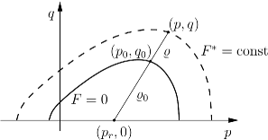
Figure 2: Implicit yield function $F^{\ast}$ generated by a convex yield surface $F=0$.

In order to evaluate the yield function $F^{\ast}(\boldsymbol{\sigma},\cdot)$ for an arbitrary stress $\boldsymbol{\sigma}$, a nonlinear equation must be solved to determine $\varrho_{0}$. That equation corresponds to the condition that the image point $(p_{0},q_{0})$ lies on the yield surface. The yield function $F^{\ast}$ is thus an implicit function. Consequently, its derivatives, for instance, the gradient used in the flow rule, involve the derivatives of the implicit dependence of $\varrho_{0}$ on the stress $\boldsymbol{\sigma}$ and, possibly, also on hardening variables. The details can be found in [17].

The present implementation of the PBG model employs the above implicit formulation of the BP yield function. Accordingly, the actual use of the implicit yield function $F^{\ast}$ and its gradient $\textbf{\em N}^{\ast}$ is denoted below by a ‘$\ast$’ in the superscript.

4.2 Incremental flow rule

With regard to finite element implementation, the constitutive equations specified in Section 3 must be cast in an incremental form, i.e., an appropriate time integration scheme must be applied to the evolution equations for internal variables.

Using the flow rule (34), the rate constitutive equation (27) is rewritten as

$$\dot{\textbf{\em T}}{}^{(2)}=\mathbbm{E}[\dot{\textbf{\em E}}{}^{(2)}-\dot{\lambda}\hat{\textbf{\em N}}{}^{\ast}],$$ (37)

which upon application of the implicit backward-Euler integration scheme yields

$$\textbf{\em T}^{(2)}_{n+1}-\textbf{\em T}^{(2)}_{n}=\mathbbm{E}_{n+1}[\textbf{\em E}^{(2)}_{n+1}-\textbf{\em E}^{(2)}_{n}-\Delta\lambda\hat{\textbf{\em N}}{}^{\ast}_{n+1}],$$ (38)

where $n+1$ and $n$ in the subscript denote, respectively, the current time $t=t_{n+1}$ and the previous time $t=t_{n}$, at which the corresponding quantities are evaluated. The incremental flow rule (38) is accompanied by the complementarity conditions,

$$F^{\ast}_{n+1}=F^{\ast}(\textbf{\em T}^{(2)}_{e,n+1},p_{c,n+1})\leq 0,\qquad\Delta\lambda\geq 0,\qquad\Delta\lambda F^{\ast}_{n+1}=0,$$ (39)

that are enforced at the end of the time increment, consistently with the backward-Euler scheme applied to integrate the rate equation (37).

Considering that arbitrary stress states can be encountered during iterative solution of the return mapping algorithm, the plastic flow direction $\hat{\textbf{\em N}}{}^{\ast}$ is modified according to

$$\hat{\textbf{\em N}}{}^{\ast}=\textbf{\em N}^{\ast}-\frac{1}{3}\,\epsilon(1-\Phi_{0})\operatorname{tr}(\textbf{\em N}^{\ast}\textbf{\em C}_{p}^{-1})\textbf{\em C}_{p},\qquad\Phi_{0}=\frac{p_{0}+c}{p_{c}+c},\qquad p_{0}=\frac{p+F^{\ast}p_{r}}{1+F^{\ast}},$$ (40)

so that $\Phi_{0}\in[0,1]$, just like $\Phi\in[0,1]$ for the stresses satisfying $F^{\ast}=0$. Of course, the flow rule is unaltered for $F^{\ast}=0$.

Remark 1.

The simple backward-Euler scheme is usually avoided in finite-strain plasticity, in particular, in the case of plastically incompressible (or nearly incompressible) materials, e.g., in metal plasticity, and integration schemes employing the exponential map are then preferable, cf. [21, 22]. However, the present plastic flow rule, formulated in terms of the inelastic strain rate $\dot{\textbf{\em E}}_{\it in}$ to consistently introduce the elastoplastic coupling, is not well suited for application of an exponential map integrator.

4.3 Constitutive update problem

In the constitutive update problem, given are the deformation gradient $\textbf{\em F}_{n+1}$ at the current time step and the internal variables $\textbf{\em C}_{p,n}$ and $p_{c,n}$ at the previous time step, and the goal is to find the current internal variables $\textbf{\em C}_{p,n+1}$ and $p_{c,n+1}$ and the plastic multiplier $\Delta\lambda$ that satisfy the incremental flow rule (38), the complementarity conditions (39) and the constitutive relationship between $p_{c,n+1}$ and $\textbf{\em C}_{p,n+1}$ specified by Eq. (25).

The second Piola–Kirchhoff stress $\textbf{\em T}^{(2)}_{n+1}$, which is needed to evaluate the yield function $F^{\ast}_{n+1}$ and its gradient $\textbf{\em N}^{\ast}_{n+1}$ in Eqs. (38)–(40), is defined by the free energy according to

$$\textbf{\em T}^{(2)}_{n+1}=2\frac{\partial\phi(\textbf{\em C}_{n+1},\textbf{\em C}_{p,n+1},p_{c,n+1})}{\partial\textbf{\em C}_{n+1}}.$$ (41)

The constitutive update problem is solved here using the classical return-mapping algorithm [1, 2]. The trial stress is first computed by assuming that the response is elastic,

$$\textbf{\em T}_{n+1}^{(2)\it trial}=2\frac{\partial\phi(\textbf{\em C}_{n+1},\textbf{\em C}_{p,n},p_{c,n})}{\partial\textbf{\em C}_{n+1}},$$ (42)

for which the trial value of the yield function is evaluated according to

$$F^{\ast\it trial}_{n+1}=F^{\ast}(\textbf{\em T}_{e,n+1}^{(2)\it trial},p_{c,n}),$$ (43)

where the necessary invariants of $\textbf{\em T}_{e,n+1}^{(2)\it trial}$ are expressed in terms of $\textbf{\em T}_{n+1}^{(2)\it trial}$ and $\textbf{\em C}_{p,n}$ using the formulae in Eq. (32).

If $F^{\ast\it trial}_{n+1}\leq 0$ then the step is elastic, and

$$\textbf{\em C}_{p,n+1}=\textbf{\em C}_{p,n},\qquad p_{c,n+1}=p_{c,n},\qquad\Delta\lambda=0.$$ (44)

If $F^{\ast\it trial}_{n+1}>0$ then the step is plastic and a set of nonlinear equations must be solved,

$${\rm\bf Q}_{n+1}({\rm\bf h}_{n+1})={\rm\bf 0},$$ (45)

where the vector of unknowns ${\rm\bf h}_{n+1}$ comprises the internal variables and the plastic multiplier $\lambda$,

$${\rm\bf h}_{n+1}=\{C_{p,11},C_{p,22},C_{p,33},C_{p,12},C_{p,13},C_{p,23},\lambda,p_{c}\}_{n+1},$$ (46)

and $C_{p,ij}$ denote the components of $\textbf{\em C}_{p}$. The local residual vector ${\rm\bf Q}_{n+1}$ is defined as

$${\rm\bf Q}_{n+1}=\{{\cal Z}_{11},{\cal Z}_{22},{\cal Z}_{33},{\cal Z}_{12},{\cal Z}_{13},{\cal Z}_{23},F^{\ast}_{n+1},{\cal A}_{n+1}\},$$ (47)

where ${\cal Z}_{ij}$ are the component-wise residuals corresponding to the incremental flow rule (38),

$${\cal Z}_{ij}=\left(\textbf{\em T}^{(2)}_{n+1}-\textbf{\em T}^{(2)}_{n}-\mathbbm{E}_{n+1}[\textbf{\em E}^{(2)}_{n+1}-\textbf{\em E}^{(2)}_{n}-\Delta\lambda\hat{\textbf{\em N}}{}^{\ast}_{n+1}]\right)_{ij},$$ (48)

and ${\cal A}_{n+1}=0$ is the equation that relates the hardening variable $p_{c,n+1}$ and the plastic strain $\textbf{\em C}_{p,n+1}$, cf. Eq. (25),

$${\cal A}_{n+1}=(\det\textbf{\em C}_{p,n+1})^{1/2}-1-{\cal H}(p_{c,n+1}).$$ (49)

Equation (45) is solved using the Newton method according to the following iterative scheme:

$${\rm\bf h}_{n+1}^{(j+1)}={\rm\bf h}_{n+1}^{(j)}+\Delta{\rm\bf h}_{n+1}^{(j)},\qquad\Delta{\rm\bf h}_{n+1}^{(j)}=-\left(\frac{\partial{\rm\bf Q}_{n+1}}{\partial{\rm\bf h}_{n+1}}\right)^{-1}{\rm\bf Q}_{n+1}({\rm\bf h}_{n+1}^{(j)}).$$ (50)

Once the constitutive update problem is solved, the first Piola–Kirchhoff stress $\textbf{\em P}_{n+1}$ and the consistent constitutive tangent $\mathbbm{C}^{\it ep}_{n+1}$ are computed,

$$\textbf{\em P}_{n+1}=\textbf{\em F}_{n+1}\textbf{\em T}^{(2)}_{n+1},\qquad\mathbbm{C}^{\it ep}_{n+1}=\frac{\partial\textbf{\em P}_{n+1}}{\partial\textbf{\em F}_{n+1}},$$ (51)

that are needed at the global level where the equilibrium equations are solved using the finite element method. It is reminded here that the internal variables ${\rm\bf h}_{n+1}$ implicitly depend on $\textbf{\em F}_{n+1}$ through Eq. (45), and the derivative of this implicit dependence must be accounted for when computing the consistent tangent $\mathbbm{C}^{\it ep}_{n+1}$, cf. [23].

In the present implementation, the standard return mapping algorithm specified above has been actually replaced by a more robust algorithm employing the augmented primal closest-point projection method proposed by Perez-Foguet and Armero [24]. This improved algorithm is described in Appendix B.

The model has been implemented using AceGen [14, 15], a symbolic code generation system that combines the symbolic capabilities of Mathematica (www.wolfram.com) with the automatic differentiation technique and additional tools for optimization and automatic generation of computer codes. The present formulation of incremental elastoplasticity and the structure of the constitutive update problem fit the general formulation introduced by Korelc [15], hence the automation approach developed in [15] can be directly applied to derive the necessary finite element routines. In particular, the incremental constitutive model is fully defined by specifying the local residual ${\rm\bf Q}_{n+1}$ in terms of the internal variables ${\rm\bf h}_{n+1}$, as done above, while the remaining part of the formulation remains unaltered. The details are omitted here; an interested reader is referred to [15], see also Section 2 in [25] for a concise presentation of the present automation approach in finite-strain elastoplasticity.

Application of the automatic differentiation technique implemented in AceGen results in the exact linearization of the incremental constitutive relationships which is highly beneficial for the overall performance of the Newton-based computational scheme applied to solve the global equilibrium equations.

It has been checked numerically that the consistent elastoplastic tangent $\mathbbm{C}^{\it ep}_{n+1}$ corresponding to the associated flow rule, i.e., for $\epsilon=0$, is not symmetric for a finite strain increment. However, the symmetry is recovered for the strain increment decreasing to zero. This shows consistency of the present incremental scheme with the rate formulation in which a symmetric elastoplastic tangent is obtained (for associative plasticity) from the Prager’s consistency condition, see [11].

5 Numerical example

An application of the model to finite element computations is presented in this section. Specifically, compaction of an alumina powder in a cylindrical die is considered with account for die-wall friction, and the effect of friction coefficient and initial aspect ratio is studied in detail. Other examples, including comparison to experimental results, can be found in [12].

Consider thus cold compression of alumina powder into a rigid cylindrical mould of radius $r$. The powder specimen has an initial height $h_{0}$ and is compressed by a rigid punch with a maximum force corresponding to the average compaction pressure of 160 MPa. Three values of the initial aspect ratio of the alumina sample are employed, $h_{0}/r=2$, $4$ and $6$. Coulomb friction is assumed at the powder-mould and powder-punch contact interfaces, and three values of the friction coefficient are used, $\mu=0.1$, $0.3$ and $0.5$. Material parameters corresponding to alumina powder are provided in Table 1, see [10, 12]. The value of parameter $\mu_{0}$ has been increased with respect to that adopted in [10, 12] since it has been noticed that the latter may lead to exceedingly large elastic shear strains. At the same time, in compression-dominated processes, such as those considered in [10, 12] and in the present paper, the overall response is not significantly affected.

Table 1: Material parameters for alumina powder.

$M$ $m$ $\alpha$ $\beta$ $\gamma$ $\epsilon$ $\tilde{a}_{1}$ $\tilde{a}_{2}$ $\Lambda_{1}$ (MPa)​​ $\Lambda_{1}$ (MPa)​​ 1.1 2 0.1 0.19 0.9 0.5 0.383 0.124 1.8 40 $c_{\infty}$ (MPa)​​ $\Gamma$ (MPa^-1)​​ $p_{cb}$ (MPa)​​ $B$ (MPa^-1)​​ $n$ $\mu_{0}$ (MPa)​​ $\mu_{1}$ $\kappa$ $e_{0}$ $p_{0}$ (MPa)​​ 2.3 0.026 3.2 0.18 6 20 64 0.04 2.129 0.063

In the finite element implementation, an axisymmetric under-integrated four-node element employing the volumetric-deviatoric split and Taylor expansion of shape functions [26] is used for the solid, and the augmented Lagrangian method used to enforce the frictional contact constraints [27, 28].

The effect of friction coefficient $\mu$ and initial aspect ratio $h_{0}/r$ is illustrated in Fig. 3 which shows the average compacting pressure as a function of the height reduction $\Delta h/h_{0}$. In each case, in addition to the compacting pressure indicated by a solid line, the corresponding average pressure at the bottom part of the mould is also shown using a dashed line of the same color. Clearly, for frictionless contact at the die wall, the two pressures would be equal one to the other, and the difference increases with increasing friction coefficient $\mu$ and with increasing initial aspect ratio $h_{0}/r$.

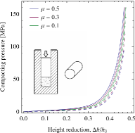
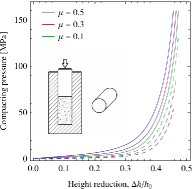
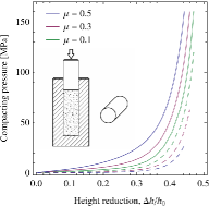
    (a)     (b)     (c)

Figure 3: The average compacting pressure (solid lines) and the average pressure at the bottom part of the mould (dashed lines) as a function of the height reduction $\Delta h/h_{0}$ for: (a) $h_{0}/r=2$, (b) $h_{0}/r=4$, (c) $h_{0}/r=6$.

The finite element mesh representing one half of the cross-section of the (axisymmetric) sample is shown in Fig. 4 for $h_{0}/r=2$ and $h_{0}/r=6$. The undeformed mesh is shown in the left column, and the deformed meshes corresponding to the maximum compression force and different friction coefficients are shown aside. The color map, identical for all figures, indicates the resulting density of alumina powder. Due to friction, the density is nonuniform within the cross-section of the specimen, and the substantial effect of friction coefficient $\mu$ and initial aspect ratio $h_{0}/r$ on the density distribution is clearly seen in Fig. 4.

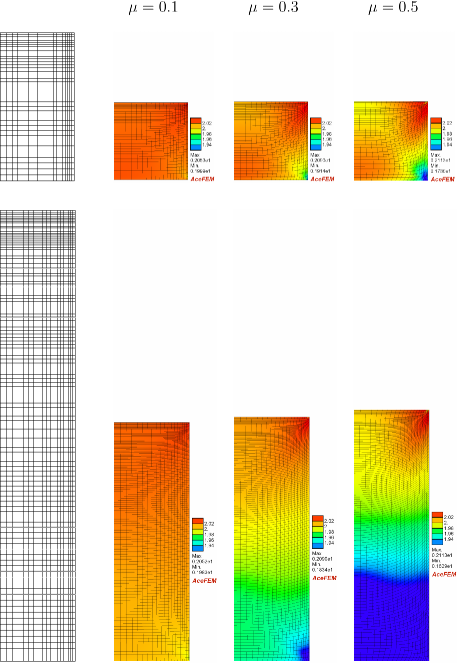
Figure 4: Axisymmetric compression into a rigid cylindrical mould: the undeformed mesh (left) and the deformed mesh corresponding to a prescribed maximum force and different friction coefficients $\mu$ for $h_{0}/r=2$ (upper row) and $h_{0}/r=6$ (lower row). The color map, identical for all figures, indicates the density $\varrho$ (in g/cm³).

The effect of friction, which is more pronounced for higher aspect ratios, results in reduced overall compaction so that the final height corresponding to the same prescribed maximum compression force depends on the friction coefficient. This is particularly visible for $h_{0}/r=6$. Also, the deformation pattern is affected by the shear stresses due to friction at the die wall, which is seen in the distortion of the initially rectangular mesh.

In the PBG model, plastic hardening is governed by the volumetric plastic deformation. Nonuniform distribution of density results thus in nonuniform hardening within the sample. This is illustrated in Fig. 5 which shows the distribution of the cohesion $c$, again indicated by the same color map for all figures. The pattern of inhomogeneity of $c$ is qualitatively similar to that shown in Fig. 4, and the same applies to the distribution of the forming pressure $p_{c}$ (not shown for brevity).

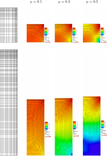
Figure 5: Axisymmetric compression into a rigid cylindrical mould: the undeformed mesh (left) and the deformed mesh corresponding to a prescribed maximum force and different friction coefficients $\mu$ for $h_{0}/r=2$ (upper row) and $h_{0}/r=6$ (lower row). The color map, identical for all figures, indicates the cohesion $c$ (in MPa).

6 Conclusion

A finite strain model for powder compaction has been developed through the derivation of an incremental scheme allowing the successful FE implementation of a series of ‘non-standard’ constitutive features, including: (i.) nonlinear elastic behaviour even at small strain; (ii.) coupling between elastic and plastic deformation; (iii.) pressure- and $J_{3}$-dependent yielding; (iv.) non-isochoric flow. The extension of concepts established at small strain to the large deformation context has required a proper selection of the stress variable to be employed for the yield function and the definition of a neo-Hookean ‘correction’ to the small strain elastic potential. An incremental scheme compatible with the finite-strain formulation of elastoplastic coupling has also been developed. The numerical tests performed on the model have indicated a correct and robust behaviour of the developed code and have demonstrated the possibility of accurate simulation of the transition from a granular material to a fully dense body occurring during the cold forming of ceramic powders.

Appendix A Free energy expressed in terms of the logarithmic elastic strain $\boldsymbol{\epsilon}_{e}$

In this appendix, we provide the formulation corresponding to the original form of the free energy function as proposed in [11]. Consider thus the small-strain free energy function (2) with the infinitesimal elastic strain $\boldsymbol{\varepsilon}_{e}$ simply replaced by the logarithmic elastic strain $\boldsymbol{\epsilon}_{e}$, viz.

$$\phi(\textbf{\em C},\textbf{\em C}_{p},p_{c})=c\,\operatorname{tr}\boldsymbol{\epsilon}_{e}+(p_{0}+c)\left[\left(d-\frac{1}{d}\right)\frac{(\operatorname{tr}\boldsymbol{\epsilon}_{e})^{2}}{2\tilde{\kappa}}+d^{1/n}\tilde{\kappa}\exp\left(-\frac{\operatorname{tr}\boldsymbol{\epsilon}_{e}}{d^{1/n}\tilde{\kappa}}\right)\right]+\mu\operatorname{tr}\boldsymbol{\epsilon}_{e}^{2}-\frac{\mu}{3}(\operatorname{tr}\boldsymbol{\epsilon}_{e})^{2}.$$ (52)

The difference with respect to the free energy function (21) concerns the shear response introduced by the last two terms in Eq. (52). We also note that, in the original form [11], the logarithmic plastic strain $\textbf{\em E}_{p}^{(0)}$ has been adopted as the internal variable rather than the plastic right Cauchy–Green tensor $\textbf{\em C}_{p}$. The two tensors are related by Eq. (20)₂, or by the inverse relationship $\textbf{\em C}_{p}=\exp(2\textbf{\em E}_{p}^{(0)})$, hence both formulations are equivalent. As shown below, explicit formulae involving $\textbf{\em C}_{p}$ are readily available, hence using $\textbf{\em E}_{p}^{(0)}$ as the internal variable would introduce an additional and unnecessary complexity related to the tensor exponential function relating $\textbf{\em E}_{p}^{(0)}$ and $\textbf{\em C}_{p}$.

The free energy (52) is expressed in terms of two invariants of the logarithmic elastic strain $\boldsymbol{\epsilon}_{e}$, namely $\operatorname{tr}\boldsymbol{\epsilon}_{e}$ and $\operatorname{tr}\boldsymbol{\epsilon}_{e}^{2}$. Evaluation of the former does not pose any difficulties, see Eqs. (23)–(24). In order to compute the second invariant, $\operatorname{tr}\boldsymbol{\epsilon}_{e}^{2}$, the logarithmic elastic strain $\boldsymbol{\epsilon}_{e}$ must be computed explicitly (this has been avoided in the case of the first invariant $\operatorname{tr}\boldsymbol{\epsilon}_{e}$). In view of Eqs. (18)₃ and (20)₁, we have

$$\boldsymbol{\epsilon}_{e}=\frac{1}{2}\log(\textbf{\em F}\textbf{\em C}_{p}^{-1}\textbf{\em F}^{T}).$$ (53)

However, this expression involves the deformation gradient F and not the right Cauchy–Green tensor C. Note that an explicit dependence on C (or equivalently on $\textbf{\em E}^{(2)}$) is needed in the present elastoplasticity framework, see Eqs. (26)–(27). Due to objectivity, the free energy function is invariant to a rigid-body rotation, hence we have

$$\operatorname{tr}\boldsymbol{\epsilon}_{e}^{2}=\operatorname{tr}(\boldsymbol{\epsilon}_{e}^{\ast})^{2},\qquad\boldsymbol{\epsilon}_{e}^{\ast}=\frac{1}{2}\log(\textbf{\em U}\textbf{\em C}_{p}^{-1}\textbf{\em U})=\frac{1}{2}\log(\textbf{\em C}^{1/2}\textbf{\em C}_{p}^{-1}\textbf{\em C}^{1/2}),$$ (54)

where $\boldsymbol{\epsilon}_{e}^{\ast}$ refers to a special configuration rotated by $\textbf{\em R}=\textbf{\em F}\textbf{\em U}^{-1}$ with respect to the current configuration. It is seen that the resulting formula (54) for $\operatorname{tr}\boldsymbol{\epsilon}_{e}^{2}$ is rather complex as it involves the tensor logarithm function and the square root of C. Even more importantly, if the above formulation was adopted, then solution of the constitutive update problem would involve the third derivative the tensor logarithm function, which would be associated with a prohibitively high computational cost.

Considering that the elastic strains are relatively small in the materials of interest, the second invariant $\operatorname{tr}\boldsymbol{\epsilon}_{e}^{2}$ can be approximated with a high accuracy by exploiting the following approximation of the logarithmic strain, see [29],

$$\boldsymbol{\epsilon}_{e}=\log\textbf{\em V}_{e}\approx\frac{1}{2}(\textbf{\em V}_{e}-\textbf{\em V}_{e}^{-1}),$$ (55)

which leads to

$$\operatorname{tr}\boldsymbol{\epsilon}_{e}^{2}\approx\frac{1}{4}(\operatorname{tr}\textbf{\em b}_{e}+\operatorname{tr}\textbf{\em b}_{e}^{-1}-6)=\frac{1}{4}[\operatorname{tr}(\textbf{\em C}\textbf{\em C}_{p}^{-1})+\operatorname{tr}(\textbf{\em C}\textbf{\em C}_{p}^{-1})^{-1}-6].$$ (56)

Concluding, the free energy function (52) can be directly expressed in terms of C and $\textbf{\em C}_{p}$ using Eq. (24) for $\operatorname{tr}\boldsymbol{\epsilon}_{e}$ and Eq. (54) or (56) for $\operatorname{tr}\boldsymbol{\epsilon}_{e}^{2}$.

Appendix B Augmented primal closest-point projection

The augmented primal closest-point projection method proposed in [24] proved to significantly improve the convergence of the Newton method used for the solution of the return-mapping equations in the constitutive update problem defined in Section 4.3. The idea is to apply the augmented Lagrangian method to enforce the inequality constraints corresponding to the incremental complementarity conditions, cf. Eq. (39),

$$F^{\ast}_{n+1}\leq 0,\qquad\Delta\lambda\geq 0,\qquad\Delta\lambda F^{\ast}_{n+1}=0.$$ (57)

The simple treatment proposed in [24] amounts to replacing the plastic multiplier $\Delta\lambda$ in the incremental flow rule (38) by the augmented one, $\Delta\hat{\lambda}$,

$$\Delta\hat{\lambda}=\max(0,\Delta\lambda+\varrho F^{\ast}_{n+1}),$$ (58)

where $\varrho>0$. The condition $F^{\ast}_{n+1}=0$ is modified accordingly,

$$\hat{F}^{\ast}_{n+1}=\frac{1}{\varrho}(\Delta\hat{\lambda}-\Delta\lambda)=0,$$ (59)

which now enforces $F^{\ast}_{n+1}=0$ when $\Delta\lambda+\varrho F^{\ast}_{n+1}>0$ and $\Delta\lambda=0$ otherwise. As a result, the local residual ${\rm\bf Q}_{n+1}$ is redefined as

$${\rm\bf Q}_{n+1}=\{{\cal Z}_{11},{\cal Z}_{22},{\cal Z}_{33},{\cal Z}_{12},{\cal Z}_{13},{\cal Z}_{23},\hat{F}^{\ast}_{n+1},{\cal A}\},$$ (60)

with ${\cal Z}_{ij}$ given by

$${\cal Z}_{ij}=\left(\textbf{\em T}^{(2)}_{n+1}-\textbf{\em T}^{(2)}_{n}-\mathbbm{E}_{n+1}[\textbf{\em E}^{(2)}_{n+1}-\textbf{\em E}^{(2)}_{n}-\Delta\hat{\lambda}\hat{\textbf{\em N}}{}^{\ast}_{n+1}]\right)_{ij},$$ (61)

Although the solution sought in the plastic state ($F^{\ast\it trial}_{n+1}>0$) corresponds to a strictly positive $\Delta\lambda$, the above simple treatment leads to a significant increase of the radius of convergence of the Newton method (actually, now a semi-smooth Newton method due to the $\max(\cdot)$ function in the definition of $\Delta\hat{\lambda}$) so that the computations may proceed with larger time increments.

References

- [1] J. C. Simo and T. J. R. Hughes. Computational Inelasticity. Springer-Verlag, New York, 1998.
- [2] E. A. de Souza Neto, D. Peric, and D. R. J. Owen. Computational Methods for Plasticity: Theory and Applications. Wiley, 2008.
- [3] R. I. Borja and C. Tamagnini. Cam-clay plasticity part iii: Extension of the infinitesimal model to include finite strains. Comput. Method. Appl. M., 155:73–95, 1998.
- [4] G. Meschke and W. N. Liu. A re-formulation of the exponential algorithm for finite strain plasticity in terms of Cauchy stresses. Comp. Meth. Appl. Mech. Engng., 173:167–187, 1999.
- [5] A. Perez-Foguet, A. Rodriguez-Ferran, and A. Huerta. Efficient and accurate approach for powder compaction problems. Comput. Mech., 30:220–234, 2003.
- [6] M. Ortiz and A. Pandolfi. A variational cam-clay theory of plasticity. Comput. Method. Appl. M., 193:27–29, 2004.
- [7] M. Rouainia and D. M. Wood. Computational aspects in finite strain plasticity analysis of geotechnical materials. Mech. Res. Commun., 33:123–133, 2006.
- [8] G. Frenning. Analysis of pharmaceutical powder compaction using multiplicative hyperelasto-plastic theory. Powder Technol., 172:103–112, 2007.
- [9] A. Karrech, K. Regenauer-Lieb, and T. Poulet. Frame indifferent elastoplasticity of frictional materials at finite strain. Int. J. Solids Struct., 48:397–407, 2011.
- [10] A. Piccolroaz, D. Bigoni, and A. Gajo. An elastoplastic framework for granular materials becoming cohesive through mechanical densification. Part I – small strain formulation. Eur. J. Mech. A/Solids, 25:334–357, 2006.
- [11] A. Piccolroaz, D. Bigoni, and A. Gajo. An elastoplastic framework for granular materials becoming cohesive through mechanical densification. Part II – the formulation of elastoplastic coupling at large strain. Eur. J. Mech. A/Solids, 25:358–369, 2006.
- [12] S. Stupkiewicz, A. Piccolroaz, and D. Bigoni. Elastoplastic coupling to model cold ceramic powder compaction. J. Eur. Cer. Soc., 2014. doi:10.1016/j.jeurceramsoc.2013.11.017.
- [13] D. Bigoni and A. Piccolroaz. Yield criteria for quasibrittle and frictional materials. Int. J. Sol. Struct., 41:2855–2878, 2004.
- [14] J. Korelc. Multi-language and multi-environment generation of nonlinear finite element codes. Engineering with Computers, 18:312–327, 2002.
- [15] J. Korelc. Automation of primal and sensitivity analysis of transient coupled problems. Comp. Mech., 44:631–649, 2009.
- [16] D. Bigoni. Bifurcation and instability of non-associative elastoplastic solids. In H. Petryk, editor, Material Instabilities in Elastic and Plastic Solids, volume 414 of CISM Courses and Lectures, pages 1–52. Springer-Verlag Wien, 2000.
- [17] S. Stupkiewicz, R. P. Denzer, A. Piccolroaz, and D. Bigoni. Implicit yield function formulation for granular and rock-like materials. (submitted).
- [18] R. Hill and J. R. Rice. Elastic potentials and the structure of inelastic constitutive laws. SIAM J. Appl. Math., 25:448–461, 1973.
- [19] R. M. Brannon and S. Leelavanichkul. A multi-stage return algorithm for solving the classical damage component of constitutive models for rocks, ceramics, and other rock-like media. Int. J. Fract., 163:133–149, 2010.
- [20] M. Penasa, A. Piccolroaz, L. Argani, and D. Bigoni. Integration algorithms of elastoplasticity for ceramic powder compaction. J. Eur. Cer. Soc. doi:10.1016/j.jeurceramsoc.2014.01.041.
- [21] G. Weber and L. Anand. Finite deformation constitutive equations and a time integration procedure for isotropic, hyperelastic–viscoplastic solids. Comp. Meth. Appl. Mech. Engng., 79:173–202, 1990.
- [22] P. Steinmann and E. Stein. On the numerical treatment and analysis of finite deformation ductile single crystal plasticity. Comp. Meth. Appl. Mech. Engng., 129:235–254, 1996.
- [23] P. Michaleris, D. A. Tortorelli, and C. A. Vidal. Tangent operators and design sensitivity formulations for transient non-linear coupled problems with applications to elastoplasticity. Int. J. Num. Meth. Engng., 37:2471–2499, 1994.
- [24] A. Perez-Foguet and F. Armero. On the formulation of the closest-point projection algorithms in elastoplasticity—part II: Globally convergent schemes. Int. J. Num. Meth. Engng., 53:331–374, 2002.
- [25] J. Korelc and S. Stupkiewicz. Closed-form matrix exponential and its application in finite-strain plasticity. Int. J. Num. Meth. Engng., 2014. doi:10.1002/nme.4653.
- [26] J. Korelc and P. Wriggers. Improved enhanced strain four-node element with Taylor expansion of the shape functions. Int. J. Num. Meth. Engng., 40:407–421, 1997.
- [27] P. Alart and A. Curnier. A mixed formulation for frictional contact problems prone to Newton like solution methods. Comp. Meth. Appl. Mech. Engng., 92:353–375, 1991.
- [28] J. Lengiewicz, J. Korelc, and S. Stupkiewicz. Automation of finite element formulations for large deformation contact problems. Int. J. Num. Meth. Engng., 85:1252–1279, 2011.
- [29] Z. P. Bazant. Easy-to-compute tensors with symmetric inverse approximating Hencky finite strain and its rate. Trans. ASME J. Eng. Mat. Technol., 120:131–136, 1998.