Modified Brans–Dicke Theory in Arbitrary Dimensions

Abstract

Within an algebraic framework, used to construct the induced–matter–theory (IMT) setting, in $(D+1)$–dimensional Brans–Dicke (BD) scenario, we obtain a modified BD theory (MBDT) in $D$ dimensions. Being more specific, from the $(D+1)$–dimensional field equations, a $D$–dimensional BD theory, bearing new features, is extracted by means of a suitable dimensional reduction onto a hypersurface orthogonal to the extra dimension. In particular, the BD scalar field in such $D$–dimensional theory has a self–interacting potential, which can be suitably interpreted as produced by the extra dimension. Subsequently, as an application to cosmology, we consider an extended spatially flat FLRW geometry in a $(D+1)$–dimensional space–time. After obtaining the power–law solutions in the bulk, we proceed to construct the corresponding physics, by means of the induced MBDT procedure, on the $D$–dimensional hypersurface. We then contrast the resulted solutions (for different phases of the universe) with those usually extracted from the conventional GR and BD theories in view of current ranges for cosmological parameters. We show that the induced perfect fluid background and the induced scalar potential can be employed, within some limits, for describing different epochs of the universe. Finally, we comment on the observational viability of such a model.

I Introduction

Models of the universe in more than four dimensions have been widely investigated. Kaluza-Klein (KK) type theories Kaluza21 ; Klein26 ; OW97 , ten–dimensional and eleven–dimensional supergravity FP12.book as well as string theories DNP86 ; GSW.book are well–known examples. Multidimensional Brane–World models, space–time–matter or IMT scenarios stm99 ; scalarbook ; 5Dwesson06 ; pav2006 in five dimensions, seeking the unification of matter and geometry, constitute other settings with additional spatial dimensions.

Unifying electromagnetism with gravity has been investigated by Kaluza by admitting Einstein general relativity (GR) in a five–dimensional space–time under three key assumptions OW97 : (i) absence of matter in higher dimensional space–time, (ii) defining the geometrical quantities exactly the same as they were in GR and (iii) omitting the derivatives with respect to the extra coordinate (cylinder condition). Since Kaluza’s procedure in 1921, compactified, projective and noncompactified versions have been studied as interesting approaches to higher dimensional unification, in which, at least one of the Kaluza’s key assumptions has been modified. Among these mentioned versions, we will consider the third. In fact, the IMT is one of these developed procedures. In the IMT, the presence of extra dimensions is also elevated to the hypothesis that matter in a four–dimensional space–time has a purely geometric origin. More precisely, it has been proposed stm99 ; 5Dwesson06 ; PW92 ; OW97 that one large extra dimension is required to obtain a consistent description, at the macroscopic level, of the properties of matter as observed in the four–dimensional space–time of GR. The IMT has been employed in the cosmological context, where concrete scenarios have been appreciated in view of recent cosmological observational data stm99 ; DRJ09 ; RJ10 . The application of the IMT framework to arbitrary dimensions has been performed in RRT95 , relating a vacuum $(D+1)$–dimensional solution to a $D$–dimensional GR space–time, with induced matter sources. This approach has also been employed to obtain lower dimensional gravity from a four–dimensional space–time description.

Another generalization of the IMT, in which the role of GR as a fundamental underlying theory is replaced by the BD theory of gravity, has also been investigated ARB07 ; Ponce1 ; Ponce2 . The BD theory is an extension of GR, in which the Newton gravitational constant is substituted, in the Jordan frame, by a non–minimally coupled scalar field BD61 ; D62 . In this latter application of the IMT, it has been shown that five–dimensional BD vacuum equations, when reduced to four dimensions, induce a modified four–dimensional BD theory. This feature is of some relevance. In fact, despite of some (“conventional”) versions of a four–dimensional BD setting, where a few assumptions have been advocated in order to obtain an accelerating cosmos, the mentioned IMT setup within a BD theory ARB07 ; Ponce1 ; Ponce2 provides a more appealing perspective based on a fundamental concept. More concretely, in the context of spatially flat Friedmann–Lemaître–Robertson–Walker (FLRW) cosmology, by employing the Wesson idea stm99 ; 5Dwesson06 ; PW92 ; OW97 for the BD theory, it has then been shown Ponce1 ; Ponce2 that the subsequent self–interacting scalar potential (geometrically due to the extra dimension) and the induced matter lead to cosmological acceleration of the matter dominated universe. Furthermore, the generalized Bianchi type I RFS11 and FLRW BFS11 models have been studied in this scenario. Our intention in this work will be to generalize the simplest scalar–tensor gravity model, the BD theory, under some of the main assumptions of the IMT, and then critical studying a spatially flat FLRW cosmological model in the extracted gravity model.

In the other reduced BD setting (different from Ponce1 ; Ponce2 ), that is also based on a fundamental concept, a five–dimensional manifold with a compact and sufficiently small fifth dimension (cylindiricity condition) has been assumed and then the five–dimensional BD equations reduced on a hypersurface orthogonal to the extra dimension qiang2005 ; qiang2009 . By assuming a few constraints especially on the matter content in five-dimensional space–time, the four–metric in this four–dimensional reduced theory is coupled with two scalar fields, which are responsible for the accelerated expansion of the universe.

In the context conveyed in the previous paragraphs, the objective of our work is to generalize the IMT formulation of the BD setting towards any arbitrary $D$–dimensional space–time. Our work is organized as follows. In Section II, we derive the BD field equations in $(D+1)$ dimensions and then, by applying a dimensional reduction procedure, within an IMT framework, we construct the MBDT on a hypersurface. Moreover, in this section, the $(D+1)$–dimensional field equations lead to a very specific $D$–dimensional BD theory, where new dynamical ingredients are present, namely, an effective induced self–interacting scalar potential. Subsequently, we investigate cosmological applications. More concretely, in Section III, we discuss exact solutions of BD cosmology in a ($D+1$)–dimensional vacuum space–time. Then, in Section IV, by means of the MBDT–IMT framework, we study the reduced $D$–dimensional cosmological solutions. We analyze them for different ranges of the equation of state parameter in a four–dimensional space-time and, subsequently, compare our results with recent constraints on the BD theory LWC13 based on the new cosmological data (e.g. Planck Planck.XVI ) as well as obtained results in the context of the standard BD theory, e.g., BP01 -BM00 . Finally, we present our conclusions in Section V. In Appendix A, we show that a $(D+1)$–dimensional BD theory can be derived from the simplest version of a KK theory in a $(D+1+d)$–dimensional space–time.

II $D$–Dimensional Brans–Dicke Theory From $(D+1)$ Dimensions

The action for the $(D+1)$–dimensional BD theory, in the Jordan frame, is written as

$${\cal S}^{{}^{(D+1)}}=\int d^{{}^{D+1}}x\sqrt{\Bigl{|}{}{\cal G}^{{}^{(D+1)}}\Bigr{|}}\,\left[\phi R^{{}^{(D+1)}}-\frac{\omega}{\phi}\,{\cal G}^{ab}\,(\nabla_{a}\phi)(\nabla_{b}\phi)+16\pi\,L\!^{{}^{(D+1)}}_{{}_{\rm matt}}\right],$$ (1)

where $\phi$ is the BD scalar field, $\omega$ is an adjustable dimensionless parameter called the BD coupling parameter, the Latin indices run from zero to $D$, $R^{{}^{(D+1)}}$ is the curvature scalar associated with the $(D+1)$–dimensional space–time metric ${\cal G}_{{ab}}$, ${\cal G}^{{}^{(D+1)}}$ is the determinant of the metric and $\nabla_{a}$ denotes the covariant derivative in $(D+1)$–dimensional space–time. The Lagrangian $L^{{}^{(D+1)}}_{{}_{\rm matt}}$ describes ordinary matter in $(D+1)$–dimensional space–time, which depends on the metric and other matter fields except on $\phi$, and we have chosen $c=1$.

The variation of action (1), with respect to the metric and the scalar field, gives the equations

$$G^{{}^{(D+1)}}_{ab}=\frac{8\pi}{\phi}\,T^{{}^{(D+1)}}_{ab}+\frac{\omega}{\phi^{2}}\left[(\nabla_{a}\phi)(\nabla_{b}\phi)-\frac{1}{2}{\cal G}_{ab}(\nabla^{c}\phi)(\nabla_{c}\phi)\right]+\frac{1}{\phi}\Big{(}\nabla_{a}\nabla_{b}\phi-{\cal G}_{ab}\nabla^{2}\phi\Big{)}$$ (2)

and

$$\frac{2\omega}{\phi}\nabla^{2}\phi-\frac{\omega}{\phi^{{}^{2}}}{\cal G}^{ab}(\nabla_{a}\phi)(\nabla_{b}\phi)+R^{{}^{(D+1)}}=0,$$ (3)

respectively, where $\nabla^{2}\equiv\nabla_{a}\nabla^{a}$ and $T^{{}^{(D+1)}}_{ab}$ is the energy–momentum tensor (EMT) of the matter fields in $(D+1)$–dimensional space–time. Contraction of the indices in Eq. (2) yields

$$R^{{}^{(D+1)}}=-\frac{16\pi\,T^{{}^{(D+1)}}}{(D-1)\phi}+\frac{\omega}{\phi^{2}}(\nabla^{c}\phi)(\nabla_{c}\phi)+\frac{2D}{D-1}\frac{\nabla^{2}\phi}{\phi},$$ (4)

where $T^{{}^{(D+1)}}={\cal G}^{ab}T^{{}^{(D+1)}}_{ab}$. By replacing (4) into (3), we further get

$$\nabla^{2}\phi=\frac{8\pi T^{{}^{(D+1)}}}{(D-1)\omega+D}.$$ (5)

In the following, by means of the reduction procedure in the context of the BD theory, we relate the $(D+1)$–dimensional field equations to the corresponding ones, with geometrically induced sources, on the $D$–dimensional space–time. Let us be more precise. We derive the reduced field equations onto a $D$–dimensional hypersurface by using the BD Eqs. (2) and (5), in a $(D+1)$–dimensional space–time described with a line element

$$dS^{2}={\cal G}_{ab}(x^{c})dx^{a}dx^{b}=g_{\mu\nu}(x^{\alpha},l)dx^{\mu}dx^{\nu}+\epsilon\psi^{2}\left(x^{\alpha},l\right)dl^{2},$$ (6)

where the Greek indices run from zero to $(D-1)$, $l$ is a non–compact coordinate associated to $(D+1)$th dimension, which is henceforth labeled with $D$. The indicator $\epsilon=\pm 1$ allows to choose the extra dimension to be either time–like or space–like, and $\psi$ is a scalar that depends on all coordinates. Choosing the line element (6) is obviously restrictive, but it is also constructive FR04 , for, as we will convey, it serves our herein purposes. We assume that the whole space–time is foliated by a family of $D$–dimensional hypersurfaces, $\Sigma$, defined by fixed values of the extra coordinate. Hence, the intrinsic metric of each hypersurface, e.g. $\Sigma_{0}$ for $l=l_{0}={\rm constant}$, is obtained by restricting the line element confined to displacements on it, being orthogonal to the $(D+1)$–dimensional unit vector

$$n^{a}=\frac{\delta^{a}_{{}_{D}}}{\psi}\qquad{\rm where}\qquad n_{a}n^{a}=\epsilon,$$ (7)

along the extra dimension Ponce1 ; Ponce2 . Thus, the induced metric $g_{\mu\nu}$ on the hypersurface $\Sigma_{0}$ has the form

$$ds^{2}={\cal G}_{\mu\nu}(x^{\alpha},l_{0})dx^{\mu}dx^{\nu}\equiv g_{\mu\nu}dx^{\mu}dx^{\nu}.$$ (8)

Now, letting $a\rightarrow\mu$ and $b\rightarrow\nu$, Eq. (2) gives the $D$–dimensional part of the corresponding $(D+1)$–quantity as

$$G_{\mu\nu}^{{}^{(D+1)}}\!\!\! = \frac{8\pi}{\phi}\,T_{\mu\nu}^{{}^{(D+1)}}+\frac{\omega}{\phi^{2}}\left[({\cal D}_{\mu}\phi)({\cal D}_{\nu}\phi)-\frac{1}{2}g_{\mu\nu}({\cal D}_{\alpha}\phi)({\cal D}^{\alpha}\phi)\right]+\frac{1}{\phi}\left[{\cal D}_{\mu}{\cal D}_{\nu}\phi-g_{\mu\nu}{\cal D}^{2}\phi\right]$$

$$- \!\!\!g_{\mu\nu}\frac{({\cal D}_{\alpha}\psi)({\cal D}^{\alpha}\phi)}{\phi\psi}+\frac{\epsilon g_{\mu\nu,}{}_{{}_{D}}\phi{}_{{}_{,D}}}{2\psi^{2}\phi}-\frac{\epsilon g_{\mu\nu}}{2\psi^{2}\phi}\left[2\phi{}_{{}_{,DD}}+\phi{}_{{}_{,D}}\left(g^{\alpha\beta}g_{\alpha\beta,}{}_{{}_{D}}-\frac{2\psi{}_{{}_{,D}}}{\psi}+\frac{\omega\phi{}_{{}_{,D}}}{\phi}\right)\right],$$

where ${\cal D}_{\alpha}$ is the covariant derivative on the hypersurface, whose computation employs $g_{\mu\nu}$. Furthermore, the notation $A{}_{{}_{,D}}$ denotes the derivative of any quantity $A$ with respect to the extra coordinate $l$, and ${\cal D}^{2}\equiv{\cal D}^{\alpha}{\cal D}_{\alpha}$. We also have used the following relations

$$(\nabla^{c}\phi)(\nabla_{c}\phi)\!\! = \!\!({\cal D}^{\alpha}\phi)({\cal D}_{\alpha}\phi)+\epsilon\left(\frac{\phi{}_{{}_{,D}}}{\psi}\right)^{2},$$ (10)

$$\nabla_{\mu}\nabla_{\nu}\phi\!\! = \!\!{\cal D}_{\mu}{\cal D}_{\nu}\phi+\frac{\epsilon\phi{}_{{}_{,D}}g_{\mu\nu,}{}_{{}_{D}}}{2\psi^{2}},$$ (11)

$$\nabla^{2}\phi\!\! = \!\!{\cal D}^{2}\phi+\frac{({\cal D}_{\alpha}\psi)({\cal D}^{\alpha}\phi)}{\psi}+\frac{\epsilon}{\psi^{2}}\left[\phi{}_{{}_{,DD}}+\phi{}_{{}_{,D}}\left(\frac{g^{\mu\nu}g_{\mu\nu,}{}_{{}_{D}}}{2}-\frac{\psi{}_{{}_{,D}}}{\psi}\right)\right].$$ (12)

To obtain the BD effective field equations on the hypersurface, we should construct the Einstein tensor on the hypersurface. Therefore, we relate the $R^{{}^{(D+1)}}_{\alpha\beta}$ and $R^{{}^{(D+1)}}$ to their corresponding quantities on the $D$–dimensional hypersurface. In this respect, we get

$$R^{{}^{(D+1)}}_{\alpha\beta}\!\!\! = \!\!\!R^{{}^{(D)}}_{\alpha\beta}-\frac{{\cal D}_{\alpha}{\cal D}_{\beta}\psi}{\psi}+\frac{\epsilon}{2\psi^{2}}\left[\frac{\psi{}_{{}_{,D}}g_{\alpha\beta,}{}_{{}_{D}}}{\psi}-g_{\alpha\beta,}{}_{{}_{DD}}-g^{\lambda\mu}g_{\alpha\lambda,}{}_{{}_{D}}g_{\beta\mu,}{}_{{}_{D}}-\frac{1}{2}g^{\mu\nu}g_{\mu\nu,}{}_{{}_{D}}g_{\alpha\beta,}{}_{{}_{D}}\right],$$ (13)

$$R^{{}^{(D+1)}}_{{}_{DD}}\!\!\! = \!\!\!-\epsilon\psi{\cal D}^{2}\psi-\frac{1}{4}g^{\lambda\beta}{}_{{}_{,D}}g_{\lambda\beta,}{}_{{}_{D}}-\frac{1}{2}g^{\lambda\beta}g_{\lambda\beta,}{}_{{}_{DD}}+\frac{1}{2\psi}g^{\lambda\beta}g_{\lambda\beta,}{}_{{}_{D}}\psi{}_{{}_{,D}}.$$ (14)

Also, by using Eqs. (2), (4), (5) and (14), we obtain

$$\frac{{\cal D}^{2}\psi}{\psi}=\!\!\!\!\! -\frac{({\cal D}_{\alpha}\psi)({\cal D}^{\alpha}\phi)}{\psi\phi}-\frac{\epsilon}{2\psi^{2}}\left[g^{\lambda\beta}g_{\lambda\beta,}{}_{{}_{DD}}+\frac{1}{2}g^{\lambda\beta}{}_{{}_{,D}}g_{\lambda\beta,}{}_{{}_{D}}-\frac{g^{\lambda\beta}g_{\lambda\beta,}{}_{{}_{D}}\psi{}_{{}_{,D}}}{\psi}\right]$$

$$-\frac{\epsilon}{\psi^{2}\phi}\left[\phi{}_{{}_{,DD}}+\phi{}_{{}_{,D}}\left(\frac{\omega\phi{}_{{}_{,D}}}{\phi}-\frac{\psi{}_{{}_{,D}}}{\psi}\right)\right]+\frac{8\pi}{\phi}\left[\frac{(\omega+1)T^{{}^{(D+1)}}}{(D-1)\omega+D}-\frac{\epsilon T^{{}^{(D+1)}}_{{}_{DD}}}{\psi^{2}}\right],$$

where the relation $g^{\mu\beta}g^{\lambda\sigma}g_{\lambda\beta,}{}_{{}_{D}}g_{\mu\sigma,}{}_{{}_{D}}+g^{\mu\sigma}{}_{{}_{,D}}g_{\mu\sigma,}{}_{{}_{D}}=0$ has been used. By applying relations (14) and (II), we can relate the Ricci scalar in $(D+1)$–dimensional space–time to its corresponding one on the hypersurface, as

$$R^{{}^{(D+1)}}=\!\!\!\!\! R^{{}^{(D)}}+\frac{2({\cal D}_{\alpha}\psi)({\cal D}^{\alpha}\phi)}{\psi\phi}-\frac{\epsilon}{4\psi^{2}}\left[g^{\alpha\beta}{}_{{}_{,D}}g_{\alpha\beta,}{}_{{}_{D}}+\left(g^{\alpha\beta}g_{\alpha\beta,}{}_{{}_{D}}\right)^{2}\right]$$

$$+\frac{2\epsilon}{\psi^{2}\phi}\left[\phi{}_{{}_{,DD}}+\phi{}_{{}_{,D}}\left(\frac{\omega\phi{}_{{}_{,D}}}{\phi}-\frac{\psi{}_{{}_{,D}}}{\psi}\right)\right]+\frac{16\pi}{\phi}\left[\frac{\epsilon T^{{}^{(D+1)}}_{{}_{DD}}}{\psi^{2}}-\frac{(\omega+1)T^{{}^{(D+1)}}}{(D-1)\omega+D}\right].$$

By using the above expressions, we can eventually obtain the reduced equations onto the $D$–dimensional hypersurface. This will produce our $D$–dimensional MBDT scenario. In what follows, we outline these retrieved equations in three separated steps, providing suitable interpretations.

Firstly, by applying equations (II), (13) and (II), we construct the Einstein equations on the hypersurface as

$$G_{\mu\nu}^{{}^{(D)}}\!\! = \!\!\frac{8\pi}{\phi}\,\left(S_{\mu\nu}+T_{\mu\nu}^{{}^{[\rm BD]}}\right)+\frac{\omega}{\phi^{2}}\left[({\cal D}_{\mu}\phi)({\cal D}_{\nu}\phi)-\frac{1}{2}g_{\mu\nu}({\cal D}_{\alpha}\phi)({\cal D}^{\alpha}\phi)\right]$$ (18)

$$+\frac{1}{\phi}\left[{\cal D}_{\mu}{\cal D}_{\nu}\phi-g_{\mu\nu}{\cal D}^{2}\phi\right]-g_{\mu\nu}\frac{V(\phi)}{2\phi}$$

$$\equiv \frac{8\pi}{\phi}T_{\mu\nu}^{{}^{(D)[{\rm eff}]}}+\frac{\omega}{\phi^{2}}\left[({\cal D}_{\mu}\phi)({\cal D}_{\nu}\phi)-\frac{1}{2}g_{\mu\nu}({\cal D}_{\alpha}\phi)({\cal D}^{\alpha}\phi)\right]+\frac{1}{\phi}\left[{\cal D}_{\mu}{\cal D}_{\nu}\phi-g_{\mu\nu}{\cal D}^{2}\phi\right]-g_{\mu\nu}\frac{V(\phi)}{2\phi}.$$ (19)

The above result conveys the standard BD equations that contain an induced scalar potential, though, there are a few points which we should make clear:

• $S_{\mu\nu}$ represents the effects of the $(D+1)$–dimensional EMT on the hypersurface and is given by

  $$S_{\mu\nu}\equiv T_{\mu\nu}^{{}^{(D+1)}}-g_{\mu\nu}\left[\frac{(\omega+1)T^{{}^{(D+1)}}}{(D-1)\omega+D}-\frac{\epsilon\,T_{{}_{DD}}^{{}^{(D+1)}}}{\psi^{2}}\right].$$ (20)

  Clearly, if one assumes that the $(D+1)$–dimensional space–time is empty of the usual matter fields [i.e., no $L_{{}_{\rm matt}}^{{}^{(D+1)}}$ term in action (2.1)], then $S_{\mu\nu}$ will vanish.

• The quantity $T_{\mu\nu}^{{}^{[\rm BD]}}$ is an induced EMT for a BD theory in $D$ dimensions and, in turn, it contains three components, namely,

  $$T_{\mu\nu}^{{}^{[\rm BD]}}=T_{\mu\nu}^{{}^{[\rm IMT]}}+T_{\mu\nu}^{{}^{[\rm\phi]}}+\frac{1}{16\pi}g_{\mu\nu}V(\phi),$$ (21)

  where

  $$\frac{8\pi}{\phi}T_{\mu\nu}^{{}^{[\rm IMT]}} \!\!\!\equiv \!\!\frac{{\cal D}_{\mu}{\cal D}_{\nu}\psi}{\psi}-\frac{\epsilon}{2\psi^{2}}\left(\frac{\psi_{{}_{,D}}g_{\mu\nu,}{}_{{}_{D}}}{\psi}-g_{\mu\nu,}{}_{{}_{DD}}+g^{\lambda\alpha}g_{\mu\lambda,}{}_{{}_{D}}g_{\nu\alpha,}{}_{{}_{D}}-\frac{1}{2}g^{\alpha\beta}g_{\alpha\beta,}{}_{{}_{D}}g_{\mu\nu,}{}_{{}_{D}}\right)$$ (23)

  $$\!\!-\frac{\epsilon g_{\mu\nu}}{8\psi^{2}}\left[g^{\alpha\beta}{}_{{}_{,D}}g_{\alpha\beta,}{}_{{}_{D}}+\left(g^{\alpha\beta}g_{\alpha\beta,}{}_{{}_{D}}\right)^{2}\right],$$

  $$\frac{8\pi}{\phi}T_{\mu\nu}^{{}^{[\rm\phi]}} \!\!\!\equiv \!\!\frac{\epsilon\phi_{{}_{,D}}}{2\psi^{2}\phi}\left[g_{\mu\nu,}{}_{{}_{D}}+g_{\mu\nu}\left(\frac{\omega\phi_{{}_{,D}}}{\phi}-g^{\alpha\beta}g_{\alpha\beta,}{}_{{}_{D}}\right)\right].$$ (24)

  The first part of the induced EMT, i.e. $T_{\mu\nu}^{{}^{[\rm IMT]}}$, is the $(D+1)$th part of the metric (6) which is geometrically induced on the hypersurface. In fact, as the BD scalar field plays (inversely) the role of the Newton gravitational constant, we can deduce that this part is the modified version of the induced EMT, introduced in the IMT scenario. Whereas, the second part, i.e. $T_{\mu\nu}^{{}^{[\rm\phi]}}$, depends on the BD scalar field and its derivatives with respect to the $(D+1)$th coordinate, has no analogue in IMT.

• The quantity introduced by $V(\phi)$ is the induced scalar potential on the hypersurface, which is derived from the other reduced equation on the hypersurface, see Eq. (II).

Secondly, we obtain the $D$–dimensional counterpart of Eq. (5), the wave equation on the hypersurface. By contracting Eq. (18), we get a relation between $R^{{}^{(D)}}$, $S=g^{\mu\nu}S_{\mu\nu}$ and $T^{{}^{[\rm BD]}}=g^{\mu\nu}T_{\mu\nu}^{{}^{[\rm BD]}}$ as

$$R^{{}^{(D)}}=-\frac{16\pi}{(D-2)\phi}\left(S+T^{{}^{[\rm BD]}}\right)+\frac{\omega({\cal D}_{\alpha}\phi)({\cal D}^{\alpha}\phi)}{\phi^{2}}+\frac{2(D-1)}{(D-2)}\frac{{\cal D}^{2}\phi}{\phi}+\frac{DV(\phi)}{(D-2)\phi}.$$ (25)

Then, by substituting relations (II) and (25) into Eq. (3) and applying relations (11) and (12), we finally achieve

$${\cal D}^{2}\phi=\frac{8\pi}{(D-2)\omega+(D-1)}\left(S+T^{{}^{[\rm BD]}}\right)+\frac{1}{(D-2)\omega+(D-1)}\left[\phi\frac{dV(\phi)}{d\phi}-\frac{D}{2}V(\phi)\right],$$ (26)

where

$$\phi\frac{dV(\phi)}{d\phi}\!\! \equiv \!\!-(D-2)(\omega+1)\left[\frac{({\cal D}_{\alpha}\psi)({\cal D}^{\alpha}\phi)}{\psi}+\frac{\epsilon}{\psi^{2}}\left(\phi_{{}_{,DD}}-\frac{\psi_{{}_{,D}}\phi_{{}_{,D}}}{\psi}\right)\right]$$

$$\!\!\!-\frac{(D-2)\epsilon\omega\phi_{{}_{,D}}}{2\psi^{2}}\left[\frac{\phi_{{}_{,D}}}{\phi}+g^{\mu\nu}g_{\mu\nu,}{}_{{}_{D}}\right]+\frac{(D-2)\epsilon\phi}{8\psi^{2}}\Big{[}g^{\alpha\beta}{}_{{}_{,D}}g_{\alpha\beta,}{}_{{}_{D}}+(g^{\alpha\beta}g_{\alpha\beta,}{}_{{}_{D}})^{2}\Big{]}$$

$$\!\!\!+8\pi(D-2)\left[\frac{(\omega+1)T^{{}^{(D+1)}}}{(D-1)\omega+D}-\frac{\epsilon\,T_{{}_{DD}}^{{}^{(D+1)}}}{\psi^{2}}\right].$$

Hence, in this applied approach, the dimensional reduction procedure provides an expression to obtain the potential, up to a constant of integration, rather than being merely introduced by hand.

Finally, we derive the counterpart equation for a conservation equation introduced within the IMT. For this purpose, by substituting $a\rightarrow\alpha$ and $b\rightarrow D$ in Eq. (2), we get

$$G_{\alpha D}^{{}^{(D+1)}}=R_{\alpha D}^{{}^{(D+1)}}=\frac{8\pi}{\phi}T^{{}^{(D+1)}}_{\alpha D}+\frac{\omega\phi_{{}_{,D}}}{\phi^{2}}({\cal D}_{\alpha}\phi)+\frac{1}{\phi}{\cal D}_{\alpha}\left(\phi_{{}_{,D}}\right)-\frac{1}{2\phi}g_{\alpha\beta,}{}_{{}_{D}}({\cal D}^{\beta}\phi)-\frac{\phi{}_{{}_{,D}}({\cal D}_{\alpha}\psi)}{\psi\phi},$$ (28)

where the first equality comes from the metric (6). On the other hand, metric (6) for the mentioned component gives

$$G^{{}^{(D+1)}}_{\alpha D}=\psi P^{\beta}{}_{\alpha;\beta},$$ (29)

where $P_{\alpha\beta}$ is given by

$$P_{\alpha\beta}\equiv\frac{1}{2\psi}\left(g_{\alpha\beta,}{}_{{}_{D}}-g_{\alpha\beta}g^{\mu\nu}g_{\mu\nu,}{}_{{}_{D}}\right).$$ (30)

Therefore, Eqs. (28) and (29) give the dynamical equation for $P_{\alpha\beta}$ as

$$P^{\beta}{}_{\alpha;\beta} = \!\!\frac{8\pi}{\psi\phi}T^{{}^{(D+1)}}_{\alpha D}+\frac{\omega\phi_{{}_{,D}}}{\psi\phi^{2}}\left({\cal D}_{\alpha}\phi\right)+\frac{1}{\psi\phi}{\cal D}_{\alpha}\left(\phi_{{}_{,D}}\right)$$ (31)

$$- \!\!\!\frac{1}{2\psi\phi}g_{\alpha\lambda,}{}_{{}_{D}}\left({\cal D}^{\lambda}\phi\right)-\frac{\phi{}_{{}_{,D}}({\cal D}_{\alpha}\psi)}{\psi^{2}\phi}\,.$$ (32)

As we conclude this section, let us further clarify a few points about the herein retrieved $D$–dimensional MBDT.

• The $(D+1)$–dimensional field equations (2) and (5), with a general metric (6), split naturally into four sets of Eqs. (II), (18), (26) and (31). As mentioned, Eqs. (18) and (26) are the BD field equations on a $D$–dimensional space–time, with a geometrically induced energy–momentum source. Such a correspondence is guaranteed by the Campbell–Magaard theorem C26 ; M63 ; RTZ95 ; LRTR97 ; SW03 . Furthermore, it is important to note that Eq. (II) has no standard BD analog, and the set of Eqs. (31) is a generalized conservation law introduced within the IMT.

• The induced EMT is covariantly conserved (the same way as in the standard four–dimensional BD theory), i.e. ${\cal D}_{\beta}T^{{}^{[\rm BD]}}_{\alpha}{}^{\beta}=0$.

• In the particular case of $D=4$ (and $L\!^{{}^{(D+1)}}_{{}_{\rm matt}}=0$), the MBDT approach reproduces the results of Ponce2 (and Ponce1 ). In addition, when $L\!^{{}^{(D+1)}}_{{}_{\rm matt}}=0$ and the BD scalar field takes constant values, the results of RRT95 are also reproduced, as expected.

• In the special case when $\omega=-1$, $l$ is a cyclic coordinate and $L\!^{{}^{(D+1)}}_{{}_{\rm matt}}=0$, the scalar potential, without loss of generality, vanishes. Thus, to reproduce a general version of a $D$–dimensional BD theory by means of the above dimensional reduction procedure, we should notice those requirements.

• In the case where $T^{{}^{(D+1)}}_{\alpha D}=0$ and the BD scalar field takes constant values, Eq. (31) reduces to $P^{{}^{(D)\beta}}{}_{\alpha;\beta}=0$. In the brane world theory, this quantity is proportional to the EMT of the matter on the brane Ponce2 ; Pon01 . If, in addition, $l$ is a cyclic coordinate then, equation (31) will reduce to an identity.

We would like to close this section by indicating an interesting point regarding how the BD theory can be related to the KK setting. An important benefit of the MBDT is that the induced matter and scalar potential, which depend on the BD scalar field and its derivatives, derived via the BD action (1), should be regarded as fundamental quantities rather than quantities added by hand. However, some questions may be asked: can we accept the BD scalar field in action (1) as a fundamental field? Where does it emerge from?

In Appendix A, by generalizing the approaches of scalarbook ; PS02 ; Faraoni.book , we show that the $(D+1)$–dimensional BD framework (in vacuum) can be derived from a generalized GR (i.e., a simplest version of the KK) theory in a $(D+1+d)$–dimensional space–time by obtaining $\omega=-1+1/d$ in which $d$ is the number of the compactified extra spatial dimensions. Moreover, in this formalism, the BD scalar field emerges as a geometrical quantity, namely, it is related to the determinant of the metric associated to submanifold of extra dimensions.

III exact solutions of BD cosmology in ($D+1$)–Dimensional vacuum space–time

In this section, we assume an empty $(D+1)$–dimensional space–time that is described by an extended version of the Friedmann–Lemaître–Robertson–Walker (FLRW) metric and then, in section (IV), by means of the MBDT procedure described in the previous section, we investigate the cosmology reduced on a $D$–dimensional hypersuface. Furthermore, in order to respect the space–time symmetries, we assume that the metric components and the BD scalar field depend only on the comoving time. Moreover, we choose the $K=0$ case with the metric

$$dS^{2}=-dt^{2}+a^{2}(t)\left[\sum^{D-1}_{i=1}\left(dx^{i}\right)^{2}\right]+\epsilon\psi^{2}(t)dl^{2},$$ (33)

where $t$ is the cosmic time, $a(t)$ and $\psi(t)$ are cosmological scale factors and $x^{i}$’s are the Cartesian coordinates.

The dynamical field equations in vacuum are given by

$$\ddot{\phi}+\dot{\phi}\left[(D-1)\frac{\dot{a}}{a}+\frac{\dot{\psi}}{\psi}\right]\!\! = \!\!0,$$ (34)

$$(D-1)\frac{\dot{a}}{a}\left(\frac{D-2}{2}\frac{\dot{a}}{a}+\frac{\dot{\psi}}{\psi}\right)\!\! = \!\!\frac{1}{\phi}\left(\ddot{\phi}+\frac{\omega}{2}\frac{\dot{\phi}^{2}}{\phi}\right),$$ (35)

$$(D-2)\frac{\ddot{a}}{a}+(D-2)\frac{\dot{a}}{a}\left[\frac{D-3}{2}\frac{\dot{a}}{a}+\frac{\dot{\psi}}{\psi}\right]+\frac{\ddot{\psi}}{\psi}\!\! = \!\!\frac{\dot{\phi}}{\phi}\left(\frac{\dot{a}}{a}-\frac{\omega}{2}\frac{\dot{\phi}}{\phi}\right),$$ (36)

$$(D-1)\left[\frac{\ddot{a}}{a}+\frac{D-2}{2}\left(\frac{\dot{a}}{a}\right)^{2}\right]\!\! = \!\!\frac{\dot{\phi}}{\phi}\left(\frac{\dot{\psi}}{\psi}-\frac{\omega}{2}\frac{\dot{\phi}}{\phi}\right),$$ (37)

where equation (34) is obtained from (5), and equations (35), (36) and (37) are associated to the components $a=0=b$, $a=b=1,2,\cdots,(D-1)$ and $a=D=b$ of Eq.(2), respectively, in which we have used equation (34). “  ${\bf\dot{}}$  ” denotes the derivative with respect to the cosmic time.

Let us solve Eqs. (34)-(37) by using the power–law solutions

$$a(t)=a_{0}\left(\frac{t}{t_{0}}\right)^{r},\hskip 28.45274pt\psi(t)=\psi_{0}\left(\frac{t}{t_{0}}\right)^{n}\hskip 14.22636pt{\rm and}\hskip 14.22636pt\phi(t)=\phi_{0}\left(\frac{t}{t_{0}}\right)^{s}\,,$$ (38)

where $a_{0}$, $\psi_{0}$ and $\phi_{0}$ are constants determined in an arbitrary fixed time $t_{0}$, and $r$, $n$ and $s$ are parameters, which are not independent, satisfying the field equations. Substituting these solutions in equations (34)–(37), it yields

$$s=1-(D-1)r-n\hskip 28.45274pt{\rm and}\hskip 28.45274pt\omega=-\frac{D(D-1)r^{2}+2(n-1)\Big{[}(D-1)r+n\Big{]}}{\Big{[}1-(D-1)r-n\Big{]}^{2}},$$ (39)

where, by assuming negative values for $n$, we must have

$$\omega\geq-\frac{n(D+1)+(D-1)}{nD+(D-2)}\hskip 28.45274pt{\rm and}\hskip 28.45274pt\omega\neq 0,-D/(D-1).$$ (40)

Some special solutions, that are of our interest, include:

• When $s$ tends to zero, then $\omega$ goes to infinity and $\phi$ takes a constant value. In this limit, the field equations are only satisfied for $r=2/D$, i.e. $n=-(D-2)/D$. Thus, the $(D+1)$–dimensional solution

  $$dS^{2}=-dt^{2}+a_{0}^{2}\left(\frac{t}{t_{0}}\right)^{\frac{4}{D}}\left[\sum^{D-1}_{i=1}\left(dx^{i}\right)^{2}\right]+\epsilon\psi_{0}^{2}\left(\frac{t}{t_{0}}\right)^{-2(D-2)/D}dl^{2}$$ (41)

  is obtained, which is the unique solution for the $(D+1)$–dimensional metric (33) for the Einstein field equations in vacuum.

• In the case where $\omega=-D/(D-1)$, we cannot set this value of $\omega$ in solutions (39) and then get the values for the exponents $r$, $n$ and $s$. However, instead, we should start from the field equations (34)–(37). It is straightforward to show that for $\omega=-D/(D-1)$, we have a $(D+1)$–dimensional de Sitter–like space

  $$a(t)=\psi(t)=a^{\prime}_{0}e^{\xi t}\qquad{\rm and}\qquad\phi(t)=\phi^{\prime}_{0}e^{-D\xi t}\,,$$ (42)

  where $\xi$, $a^{\prime}_{0}$ and $\phi^{\prime}_{0}$ are constants.

• One of the most well–known class of solutions in standard BD theory is the O’Hanlon and Tupper solution o'hanlon-tupper-72 . This class corresponds to “vacuum” with a free scalar and the range of the BD parameter in four–dimensional space–time is restricted to $\omega>-3/2$, $\omega\neq 0,-4/3$ Faraoni.book . Assuming $a(t)=\psi(t)=a_{0}\left(t/t_{0}\right)^{r}$ and $\omega\neq-D/(D-1)$ at the beginning, thus solutions (38) and (39) are reduced to a generalized O’Hanlon and Tupper solution in a ($D+1$)–dimensional space–time as

  $$dS^{2}=-dt^{2}+a_{0}^{2}\left(\frac{t}{t_{0}}\right)^{2r}\left[\sum^{D-1}_{i=1}\left(dx^{i}\right)^{2}+dl^{2}\right],\hskip 28.45274pt\phi(t)=\phi_{0}\left(\frac{t}{t_{0}}\right)^{s}$$ (43)

  where

  $$r_{\pm}=\frac{1}{(D+1)+D\omega}\left[\omega+1\pm\sqrt{\frac{(D-1)\omega+D}{D}}\right]$$ (44)

  and

  $$s_{\pm}=\frac{1\mp\sqrt{D}\sqrt{D+(D-1)\omega}}{(D+1)+D\omega}\,,$$ (45)

  where $\omega>-D/(D-1)$ and $r_{\pm}$ and $s_{\pm}$ algebraically are related by constraint $s+Dr=1$. We also assumed $\epsilon=1$. When the cosmic time goes to zero, this solution has a big bang singularity. In a four–dimensional space–time, this solution has been obtained by means of different methods o'hanlon-tupper-72 ; KE95 ; MW95 ; Faraoni.book . We can easily show that

  $$\omega=\frac{1-s}{Ds^{2}}\Big{[}(D+1)s+(D-1)\Big{]}.$$ (46)

  When $s$ tends to zero, then $\omega$ goes to infinity and $\phi$ takes a constant value. In this limit, we have

  $$dS^{2}=-dt^{2}+a_{0}^{2}t^{\frac{2}{D}}\left[\sum^{D-1}_{i=1}\left(dx^{i}\right)^{2}+dl^{2}\right].$$ (47)

  We should note that in the mentioned limit, the corresponding general relativistic solution is not reproduced; as (47) illustrates, it is not a Minkowski space. Let us check it for, e.g., a four–dimensional space–time (i.e. by setting $D=3$). In this special case, the solutions are reduced to

  $$a(t)=a_{0}\left(\frac{t}{t_{0}}\right)^{1/3}\qquad{\rm and}\qquad\phi={\rm constant},$$ (48)

  where the scale factor has a decelerated expanding behavior Faraoni.book ; RFK11 .

In the next section, as an application of the MBDT in cosmology, we proceed to investigate the effective $D$–dimensional picture generated by the exact power–law solutions in $(D+1)$–dimensional space–time.

IV Reduced Brans–Dicke Cosmology in $D$ Dimensions

The non–vanishing components of the induced EMT (21) associated to the metric (33) on the hypersurface $\Sigma_{0}$ are

$$\frac{8\pi}{\phi}T^{0[{\rm BD}]}_{\,\,\,0}\!\!\! = \!\!\!-\frac{\ddot{\psi}}{\psi}+\frac{V(\phi)}{2\phi},$$ (49)

$$\frac{8\pi}{\phi}T^{i[{\rm BD}]}_{\,\,\,i}\!\!\! = \!\!\!-\frac{\dot{a}\dot{\psi}}{a\psi}+\frac{V(\phi)}{2\phi},$$ (50)

where the induced potential $V(\phi)$ will be determined from (II). As the different components of $T^{i[{\rm BD}]}_{\,\,\,i}$ [where $i=1,2,\cdots,(D-1)$ with no sum] are equal, thus the induced–matter can be considered as a perfect fluid with an energy density $\rho_{{}_{\rm BD}}\equiv-T^{0[{\rm BD}]}_{\,\,\,0}$ and isotropic pressures $p_{{}_{\rm BD}}=p_{i}\equiv T^{i[{\rm BD}]}_{\,\,\,i}$.

In order to derive the induced scalar potential, we substitute the power–law solutions (38) into (II) and evaluate it on the hypersurface. Thus, we get

$$\phi\frac{dV}{d\phi}{\Biggr{|}}_{{}_{\Sigma_{o}}}\!\!\!\!\!=(D-2)(\omega+1)nst_{0}^{-2}\phi_{0}^{2/s}\phi^{\frac{s-2}{s}},$$ (51)

where $t_{0}$, $\phi_{0}$, $n$, $s$ and $\omega$ are given by relations (38) and (39). By integrating this equation, we obtain

$$V(\phi)=\left\{\begin{array}[]{c}\frac{2\phi_{0}}{t_{0}^{2}}(D-2)n\left(\omega+1\right){\rm ln}\phi\hskip 56.9055pt{\rm for}\hskip 14.22636pts=2\\ \\ \frac{\phi_{0}^{2/s}ns^{2}}{t_{0}^{2}(s-2)}(D-2)(\omega+1)\phi^{(s-2)/s}\hskip 42.67912pt{\rm for}\hskip 14.22636pts\neq 0,2,\\ \end{array}\right.$$

where the constants of integration have been set equal to zero. In the special cases, regardless of $D$, where $\omega=-1$ or $n=0$, the scalar potential will be zero. Also, for the particular case of $s=0$ where the BD scalar field takes constant values, it is straightforward to show that $\frac{dV}{d\phi}{\Biggr{|}}_{{}_{\Sigma_{o}}}$ identically vanishes, and thus, without loss of generality, we can set $V=0$ in this case. From now on, we will not investigate the logarithmic potential with $s=2$, for it leads to some difficulties when the weak energy condition is applied.

By substituting the scalar potential (for $s\neq 0,2$) and also the power–law solutions (38) into relations (49) and (50), we get the induced quantities in a $D$–dimensional hypersurface as

$$\rho_{{}_{\rm BD}}=\frac{\phi_{0}}{16\pi t_{0}^{s}}\frac{n\left[2(n-1)(s-2)-(D-2)(\omega+1)s^{2}\right]}{(s-2)}t^{s-2}$$ (52)

and

$$p_{{}_{\rm BD}}=-\frac{\phi_{0}}{16\pi t_{0}^{s}}\frac{n\left[2r(s-2)-(D-2)(\omega+1)s^{2}\right]}{(s-2)}t^{s-2},$$ (53)

which, by applying (39), we have

$$\rho_{{}_{\rm BD}}=-\frac{\phi_{0}}{16\pi t_{0}^{{}^{[1-(D-1)r-n]}}}\frac{(D-1)nr[(D-2)r-2n+2]+(D-4)n(n^{2}-1)}{[(D-1)r+n+1]t^{{}^{[(D-1)r+n+1]}}}$$ (54)

and

$$p_{{}_{\rm BD}}=\frac{\phi_{0}}{16\pi t_{0}^{{}^{[1-(D-1)r-n]}}}\frac{(D-1)(D-4)nr^{2}+n(n+1)[(D-2)(n-1)-2r]}{[(D-1)r+n+1]t^{{}^{[(D-1)r+n+1]}}}.$$ (55)

It is straightforward to show that the conservation law for the above induced EMT is satisfied, as expected. Consequently, from relations (54) and (55), the equation of state for the power–law solutions on the $D$–dimensional hypersurface is

$$p_{{}_{\rm BD}}=W_{{}_{\rm BD}}\rho_{{}_{\rm BD}},\hskip 28.45274ptW_{{}_{\rm BD}}\equiv-\frac{(D-1)(D-4)r^{2}-(n+1)[2r-(D-2)(n-1)]}{(D-1)r[(D-2)r-2(n-1)]+(D-4)(n^{2}-1)}.$$ (56)

We proceed to discuss cosmological consequences for different types of matter. Hence, it will be appropriate to express the parameter $r$ in terms of the deceleration parameter $q=-a\ddot{a}/(\dot{a})^{2}$, namely

$$r=\frac{1}{q+1}.$$ (57)

In order to proceed and analyze the induced quantities on the hypersurface, we should express the exponent associated to the scalar $\psi$, the scale factor of the $(D+1)$th dimension, in terms of $W_{{}_{\rm BD}}$, $r$ and $D$. Thus, from relation (56), we get

$$n=\frac{r[(D-1)W_{{}_{\rm BD}}+1]\pm\sqrt{\Delta}/2}{(D-4)W_{{}_{\rm BD}}+(D-2)},$$ (58)

where

$$\Delta\equiv \!\!\!+\!\!\! 4r^{2}\Big{[}(D-1)W_{{}_{\rm BD}}+1\Big{]}-4\Big{[}(D-4)W_{{}_{\rm BD}}+(D-2)\Big{]}$$ (59)

$$\times\Bigg{\{} \!\!\!\Big{[}\!\!\! (D^{2}-3D+2)W_{{}_{\rm BD}}+(D^{2}-5D+4)\Big{]}r^{2}+2\Big{[}(D-1)W_{{}_{\rm BD}}-1\Big{]}r+\Big{[}(4-D)W_{{}_{\rm BD}}+2-D\Big{]}\Bigg{\}},$$

where $W_{{}_{\rm BD}}$ and $D$ must be accurately set, such that we always have $\Delta\geq 0$ and a non–vanishing value for the denominator of (58). In addition, the resulted value for $n$ should give positive values for the induced energy density.

Consequently, let us re–write the reduced BD cosmological power–law solution on a $D$–dimensional hypersurface as

$$ds^{2} \equiv dS^{2}{\Big{|}}_{{}_{\Sigma_{o}}}=-dt^{2}+a_{0}^{2}\left(\frac{t}{t_{0}}\right)^{2r}\left[\sum^{D-1}_{i=1}\left(dx^{i}\right)^{2}\right],$$

$$\phi = \phi_{0}\left(\frac{t}{t_{0}}\right)^{[1-(D-1)r-n]},$$

$$V(\phi) = \frac{n(D-2)\left[(D-1)r^{2}+n^{2}-1\right]}{\left[(D-1)r+n+1\right]t_{0}^{2}\phi_{0}^{{}^{2/[(D-1)r+n-1]}}}\phi^{[(D-1)r+n+1]/[(D-1)r+n-1]},$$

$$\rho_{{}_{\rm BD}} = -\frac{\phi_{0}}{16\pi t_{0}^{{}^{[1-(D-1)r-n]}}}\frac{(D-1)nr[(D-2)r-2n+2]+(D-4)n(n^{2}-1)}{[(D-1)r+n+1]t^{{}^{[(D-1)r+n+1]}}},$$ (60)

where $n$, as a function of the parameters $W_{{}_{\rm BD}}$, $r$ and $D$, is given by (58). The constant $\phi_{0}$ has been assigned to the value of the BD scalar field at some arbitrary fixed time $t_{0}$.

In order to study accelerating solutions (in particular for late times) we further discuss the energy density and the pressure associated to the BD scalar field. From (18) and (33), the FLRW equations on a $D$–dimensional hypersurface can be written as

$$\frac{(D-1)(D-2)}{2}H^{2}\!\! = \!\!\frac{1}{\phi}\left(8\pi\rho_{{}_{\rm BD}}+\rho_{\phi}\right),$$ (61)

$$(D-2)\frac{\ddot{a}}{a}+\frac{(D-2)(D-3)}{2}H^{2}\!\! = \!\!-\frac{1}{\phi}\left(8\pi p_{{}_{\rm BD}}+p_{\phi}\right),$$ (62)

where $H=\dot{a}/a$ is the Hubble expansion rate of the universe, $\rho_{{}_{\rm BD}}$ and $p_{{}_{\rm BD}}$ are given by (54) and (55), respectively, and the energy density and pressure of the BD scalar field T02 are given by

$$\rho_{\phi}\!\! \equiv\!\! \frac{\omega}{2}\frac{\dot{\phi}^{2}}{\phi}+\frac{V(\phi)}{2}-(D-1)H\dot{\phi},$$ (63)

$$p_{\phi}\!\! \equiv\!\! \frac{\omega}{2}\frac{\dot{\phi}^{2}}{\phi}-\frac{V(\phi)}{2}+\ddot{\phi}+(D-2)H\dot{\phi}.$$ (64)

Employing (38), we get

$$\rho_{\phi}=\frac{\phi_{0}}{t_{0}^{s}}\frac{s\left[\omega s(s-2)+(D-2)(\omega+1)ns-2(D-1)(s-2)r\right]}{2(s-2)}t^{s-2}$$ (65)

and

$$p_{\phi}=\frac{\phi_{0}}{t_{0}^{s}}\frac{s\left[\omega s(s-2)-(D-2)(\omega+1)ns+2(D-2)(s-2)r+2(s-1)(s-2)\right]}{2(s-2)}t^{s-2},$$ (66)

in which the equation of state for the BD scalar field is described by

$$p_{\phi}=W_{\phi}\rho_{\phi}\hskip 14.22636pt{\rm where}\hskip 14.22636ptW_{\phi}\equiv\frac{\omega s(s-2)-(D-2)(\omega+1)ns+2(D-2)(s-2)r+2(s-1)(s-2)}{\omega s(s-2)+(D-2)(\omega+1)ns-2(D-1)(s-2)r}.$$ (67)

Equation (61) can be written in the form $\Omega_{{}_{\rm BD}}+\Omega_{\phi}=1$, with

$$\Omega_{{}_{\rm BD}} \equiv \frac{16\pi}{(D-1)(D-2)}\frac{\rho_{{}_{\rm BD}}}{H^{2}\phi},$$ (68)

$$\Omega_{\phi} \equiv \frac{2}{(D-1)(D-2)}\frac{\rho_{\phi}}{H^{2}\phi},$$

where $\Omega_{{}_{\rm BD}}$ and $\Omega_{\phi}$ are the density parameters associated to the reduced matter and the BD scalar field, respectively. By employing (38), (52), (65), the density parameters are written as

$$\Omega_{{}_{\rm BD}} = \frac{n\left[2(n-1)(s-2)-(D-2)(\omega+1)s^{2}\right]}{(D-1)(D-2)(s-2)r^{2}},$$ (69)

$$\Omega_{\phi} = \frac{s\left[\omega s(s-2)+(D-2)ns(\omega+1)-2r(D-1)(s-2)\right]}{(D-1)(D-2)(s-2)r^{2}}.$$

As the main purpose of the IMT framework is to show that the matter in the universe has a geometrical origin stm99 ; in the following subsections, we will examine the $D$–dimensional solutions for some values of $W_{{}_{\rm BD}}$. In order to compare the resulted solutions with the ones obtained in the conventional BD theory (with or without any scalar potential or other generalization, e.g. a variable BD coupling parameter), as well as with observational data, somewhere, we will restrict ourselves to $D=4$.

IV.1 Modified Brans–Dicke Cosmology and Quintessence

The observational data have shown that we are living in an accelerated expanding universe. A lot of cosmological quintessence models of dark energy (see e.g. PB99 ; T02 ; Faraoni.book ; P13 and references therein), have been presented to explain the present epoch of the universe. Scalar-tensor models of dark energy have been known as extended quintessence FJ06 . As the most of the mentioned models based on the phenomenological basis, thus, many endeavors also have been done to extract this property for the universe from fundamental physics. For instance, in several investigations, when the conventional BD theory has been used in quintessential scenarios, a scalar potential has been included by hand. As we assert that the MBDT, and in turn the induced scalar potential, is constructed based on fundamental principles, one of the aims of the MBDT is to present a model to explain the accelerated expansion. In the following subsections, we would like to examine the MBDT cosmology for describing the various epoches of the universe.

For an accelerating universe, from the power–law solution (38), we must have $r>1$. Besides, we assume the equation of the state parameter of the baroscopic matter is restricted to be between $0$ and $1$. Thus, from (56) with $D=4$, we get $-1<n<r-1$ or equivalently, from (39), we have $2-4r<s<2-3r$, which implies that $s$ is always negative. As we are interested in a shrinking fifth dimension, we would like to restrict the solutions to only negative values of $n$, namely, we take $-1<n<0$, which gives $1-3r<s<2-3r$. Furthermore, in order to satisfy the positivity conditions for $\rho_{{}_{\rm BD}}$ and $\rho_{\phi}$, from relations (52) and (65), and the resulted negative values for $s$ and $n$, the BD coupling parameter must be restricted as

$$\frac{2(1-s)}{s}<\omega<\left[\frac{(3r+s)(2-s)}{s^{2}}-1\right],\hskip 14.22636pt{\rm with}\hskip 14.22636pt1-3r<s<2-3r,$$ (70)

or equivalently, from relation (39), we get

$$\frac{2(3r+n)}{1-3r-n}<\omega<\left[\frac{(1-n)(1+3r+n)}{(1-3r-n)^{2}}-1\right],\hskip 14.22636pt{\rm with}\hskip 14.22636pt-1<n<0.$$ (71)

According to the above relations, in Fig. 1, the allowed region for the BD coupling parameter, (the region between the two hypersurfaces) has been specified versus $n$ and $r$ for an accelerated expansion.

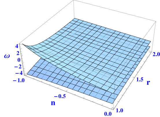
Figure 1: The region between two hypersurfaces shows the allowed region for $\omega$ versus $n$ and $r$ (the permitted values) for an accelerated expansion.

This figure has been plotted by respecting $r>1$ and the weak energy condition of the matter associated to the BD scalar field and the induced matter. In the following figures, we will find a few allowed ranges for the parameters of the model, which not only do they respect to the mentioned physical conditions, but also match with the recent observational data for the BD theory LWC13 .

By employing Eqs. (39) with $D=4$, we have obtained $W_{\phi}$ versus $n$ and $r$, and then specified an allowed range for it, numerically. As a sample, Fig. 2 gives an acceptable ranges for $W_{\phi}$ which may in agreement with the recent observational data describing the current accelerated universe. Especially, this figure also indicates that the obtained ranges for $W_{\phi}$ as well as $r$ are in accordance with the results of conventional BD theory SS01 ; SS03 .

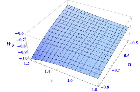
Figure 2: Resulted ranges for $W_{\phi}$ versus $r$ and $n$ in their corresponding allowed ranges.

In the other numerical endeavors, we have tried to find allowed ranges for the BD coupling parameter. In this manner, we have used the recent data for the present parameters in the model. The results of our study have shown that the best range for the BD coupling parameter is almost constrained as $-3/2<\omega<-2$. For instance, in Fig. 3, we have plotted $\omega$ versus $r$ for an allowed value of $n$. This result is also in accordance with the consequences obtained by the mentioned conventional BD theory.

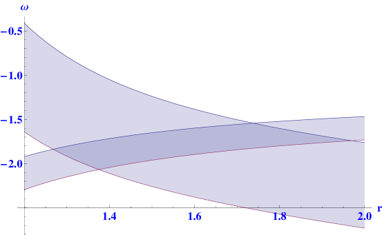
Figure 3: The overlap of the two spaces shows the allowed region in the $(r,\omega)$ parameter space for $n=-0.9$, $0.3<\Omega_{{}_{\rm BD}}<0.5$ and $-0.6<W_{\phi}<-0.8$.

Since in scalar–tensor theories, the gravitational constant is varying with time, the gravitational coupling (in the Jordan frame) is constrained by the gravitational experiments. From the effective BD action on the hypersurface, the Newton’s gravitational constant is read as the inverse of the BD scalar field, $G_{\rm N}=\phi^{-1}$. However, $G_{\rm N}$ cannot be interpreted, physically, the same as Newton’s gravitational constant in GR. In fact, it is included in the Newton force (as determined by Cavendish–type experiments) as $G_{\rm eff}m_{1}m_{2}/r_{12}^{2}$ in which $m_{1}$ and $m_{2}$ are two close test masses and $r_{12}$ is their distance. Hence, the effective gravitational constant in the BD theory (in the weak field limit) is given by $G_{\rm eff}=\phi^{-1}(2\omega+4)/(2\omega+3)$ EP01 ; NP07 . Thus, the rate of variation of $G_{\rm N}$ and $G_{\rm eff}$ have the same value and, the recent experimental limits LWC13 have shown that, at present time, it reads

$$\left[\frac{\dot{G}_{\rm eff}}{G_{\rm eff}}\right]_{t=t_{0}}\approx 1.42\times 10^{-13}yr^{-1},$$ (72)

where $t_{0}$ is the age of the universe. In our model, we have

$$\left[\frac{\dot{G}_{\rm eff}}{G_{\rm eff}}\right]_{t=t_{0}}=-\frac{s}{t_{0}}=-\frac{s}{r}H_{0},$$ (73)

where $H_{0}=r/t_{0}$ is the Hubble parameter at present. Therefore, the parameters $s$ and $r$, for an accelerated expansion at late times, should satisfy the constraint (72). If we assume that the age of the universe to be $13.7179$ Gyrs (as a best fit value), as estimated in LWC13 , thus in our model, $H_{0}t_{0}=r$ may approach to one. On the other hand, for a four–dimensional space–time, from (38), (52) and (68), we have

$$(H_{0}t_{0})^{2}=\frac{n\left[(n-1)(1+3r+n)+(\omega+1)(1-3r-n)^{2}\right]}{3(1+3r+n)\Omega_{{}_{\rm BD}}}.$$ (74)

In Fig. 4, $H_{0}t_{0}$ has been plotted versus $n$ (in the allowed range) for some allowed values of $\omega$ and $r$. As it is seen, in the permissable ranges of the parameters of the model, all the curves associated to $H_{0}t_{0}$ intersect at least once the line associated to constant values of $r=1.25$ and also $r=1.40$.

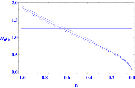
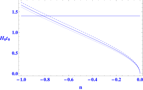
Figure 4: $H_{0}t_{0}$ versus $n$ with $r=1.25$ (left figure) and $r=1.40$ (right figure) for $\omega=-2$ (the dashed curve), $\omega=-1.8$ (the solid curve) and $\omega=-1.65$ (the dotted curve). We set $\Omega_{{}_{\rm BD}}=0.3048$.

IV.2 Matter–Dominated Universe

For a matter–dominated universe, we set $W_{{}_{\rm BD}}=0$, thus relations (58) and (59) reduce to

$$n=\frac{r\pm\sqrt{\Delta_{\rm matt}}}{(D-2)}\hskip 14.22636pt{\rm with}\hskip 14.22636pt\Delta_{\rm matt}\equiv-\left[D(D^{2}-7D+14)-9\right]r^{2}+2(D-2)r+(D-2)^{2}.$$ (75)

Therefore, by substituting these values of $n$ into solution (60), we obtain the solutions associated with a matter–dominated universe, in which all of the induced quantities are in terms of the parameters $D$ and $r$. Let us investigate the solutions for a four–dimensional space–time. By substituting $D=4$ into relation (75), we get

$$n=\frac{1}{2}(r\pm|r+2|),$$ (76)

where it yields $n=-1,r+1$. As the case where $n=r+1$ gives $\rho=0$ (for $D=4$), it is not acceptable. In what follows, we derive the solution for the case where $n=-1$.

By substituting $n=-1$ and $D=4$ into relations (39) and (60) we obtain

$$s = 2-3r,\hskip 76.82243pt\omega=-\frac{4(3r^{2}-3r+1)}{(2-3r)^{2}}$$ (77)

$$\rho = \frac{\phi_{0}(r+2)}{8\pi t_{0}^{2}}\left(\frac{t}{t_{0}}\right)^{-3r},\hskip 19.91692ptV=-\frac{2\phi_{0}r}{t_{0}^{2}}\left(\frac{t}{t_{0}}\right)^{-3r}.$$

In a particular case where $\mid\omega\mid$ tends to infinity, we obtain $r=2/3$ and thus $s=0$. Namely, in this case, the BD scalar field takes constant values and, without loss of generality, from (60), we can assume $V=0$, which implies that the usual spatially flat FLRW cosmology (for a matter–dominated universe) in the context of GR has been recovered. Besides, $n=-1$ indicates that the extra dimension contracts as the cosmic time increases.

Let us proceed to probe the general solutions without assuming any particular value for $\omega$. From relations (57) and (60), the decelerated parameter can be written in terms of $\omega$ as

$$q=\frac{1+\omega\pm\sqrt{-3(1+\omega)}}{2(1+\omega)},$$ (78)

which implies that, in order to get real values for $q$ (or $r$), the BD coupling parameter must be restricted to $\omega<-1$. Also, expressing the above relation in terms of $r$ leads to the other restriction on the BD coupling parameter, namely, $\omega\neq-4/3$. On the other hand, from relations (52) and (65), the positivity condition for $\rho_{{}_{\rm BD}}$ and $\rho_{\phi}$, in the case where $n=-1$ and $r>1$, are given by

$$-\frac{2(3r-1)}{3r-2}<\omega<\frac{6r}{(2-3r)^{2}}-1.$$ (79)

Thus, according to the above physical conditions, we have plotted this range of the BD coupling parameter versus $r$ in Fig. 5. We should mention that this specified range of $\omega$ satisfies the weak energy conditions for the matter associated to the BD scalar field and the induced matter. In addition, we notice that the obtained range of the $\omega$ is applicable to produce values for $q$ which are in agreement with the current observed measurements for the present epoch of the universe, namely, $q=-0.67\pm 0.25$.

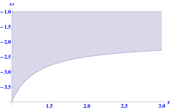
Figure 5: The allowed range of the BD coupling parameter in $(r,\omega)$ parameter space for $n=-1$ and small values of $r$ for a matter–dominated universe.

As $n=-1$, note that while the usual spatial dimensions expand with $t$, the extra dimension contracts.

In Fig. 6, we have shown $W_{\phi}$ versus $r$ for a particular value of the BD coupling parameter in the permissable range. This figure indicates that if any permissable value of $\omega$ is taken, then for small values of $r$, the value of $W_{\phi}$ can be consistent with the recent observational data.

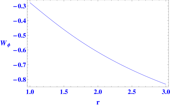
Figure 6: $W_{\phi}$ versus $r$ for $\omega=-1.49$ for the matter dominated epoch.

In order to show that the cosmology based on MBDT can work, appropriately, as an unified model for describing dark matter–dark energy, besides the above resulted solutions for only $r>1$, let us apply the following approach for explaining the consequences associated to the other values of $r$.

From equations (61) and (62), we get

$$\frac{\ddot{a}}{a}=-\frac{1}{(D-1)(D-2)\phi}\Big{[}(D-3)\rho_{{}_{\rm tot}}+(D-1)p_{{}_{\rm tot}}\Big{]},$$ (80)

where $\rho_{{}_{\rm tot}}=8\pi\rho_{{}_{\rm BD}}+\rho_{\phi}$ and $p_{{}_{\rm tot}}=8\pi p_{{}_{\rm BD}}+p_{\phi}$. As we have assumed $\phi>0$, the sign of $(D-3)\rho_{{}_{\rm tot}}+(D-1)p_{{}_{\rm tot}}$ determines to have whether accelerating or decelerating expansion (contraction). Let us focus on the the specific case of this subsection. Therefore, by using the relations (39), (52), (53), (65), (66) and setting $D=4$ and $n=-1$ in equation (80), we easily find that $\ddot{a}/a<0$ for $-1<s<2$ (except $s=0$) and $\ddot{a}/a>0$ for $s<-1$. Namely, the former case gives a decelerating expansion while the latter one gives an accelerating expansion for the universe. Note that when $s>2$, we have also $\ddot{a}/a>0$, but in this case, we have an accelerating contraction. Moreover, we have $\ddot{a}/a=0$ (zero acceleration) when $s=-1$ which corresponds to $r=1$ and $\omega=-4$. For the case where $s=2$, we get $r=0$ that yields a static universe. For both the ranges $-1<s<2$ and $s<-1$, we get $\rho_{{}_{\rm tot}}>0$ whilst, as Figure 7 shows, $\omega$ takes small negative values such that the allowed ranges (of $\omega$) are almost the same for both of the branches. Note that in this figure, when $s$ tend to zero then $|\omega|$ takes very large values. Hence, $\phi$ takes constant values and, consequently, the corresponding solutions in the IMT is recovered.

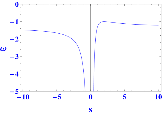
Figure 7: $\omega$ versus $s$ for $n=-1$. The right branch corresponds to a decelerating expansion and the left one corresponds to an accelerating expansion. When $s$ goes to zero, then the corresponding IMT solution is recovered.

Although the observational viability of the case $s<-1$ (which corresponds to $r>1$) has already been discussed, but, once again we note that, when $s$ is restricted to the range $s<-1$, then the deceleration parameter is restricted to $-1<q<0$, while for $-1<s<2$, it takes positive values. We should note that, in the phenomenological models based on the BD theory, the scalar potential is imposed by hand. Instead, in our model, the induced scalar potential is automatically procreated by the geometry of the extra dimension. and is responsible for describing each epoch.

IV.3 Radiation–Dominated Universe

For the radiation–dominated case in a $D$–dimensional hypersurface, we set $W_{{}_{\rm BD}}=1/(D-1)$ in (58) which gives

$$n=\frac{2(D-1)r\pm\sqrt{\Delta_{\rm rad}}}{D(D-2)-2}\hskip 14.22636pt{\rm with}\hskip 14.22636pt\Delta_{\rm rad}\equiv D^{2}(D-4)\left[D-(D-2)(D-1)r^{2}\right]+8D+4.$$ (81)

In the special case where $D=4$, relation (81) gives $n=r\pm 1$. As mentioned, the case $n=r+1$ is not acceptable. In the following, we explain the solutions associated to $n=r-1$.

By using (39) and (60) for this case, we obtain

$$s = 2(1-2r),\hskip 71.13188pt\omega=-\frac{5r-2}{2(2r-1)},$$ (82)

$$\rho = \frac{3\phi_{0}(1-r)}{16\pi t_{0}^{2}}\left(\frac{t}{t_{0}}\right)^{-4r},\hskip 19.91692ptV=\frac{\phi_{0}(1-r)(1-2r)}{t_{0}^{2}}\left(\frac{t}{t_{0}}\right)^{-4r}$$

For large values of the BD coupling parameter, we get $r=1/2$ and then, $n=-1/2$ and $s=0$, namely

$$a(t)\propto t^{1/2},\hskip 28.45274ptp(t)=3\rho(t)\propto t^{-2}\hskip 28.45274pt{\rm and}\hskip 28.45274pt\phi={\rm constant}.$$ (83)

Therefore, for the large values of $\mid\omega\mid$, a radiation–dominated epoch evolves the same way as the corresponding one of the flat FLRW space–time in GR. Also the extra dimension contracts as $t$ increases.

We further see that for $0<r<1$, and $r\neq 1/2$, the relations (52) and (65) indicate that for satisfying the weak energy conditions, $\omega$ must be restricted to $(4r-1)/(1-2r)<\omega<(-5r^{2}+6r-1)/(1-2r)^{2}$, in which for $r<1/2$, $\omega$ always takes positive values, while for $r>1/2$, it can be positive or negative. Namely, for the case $n=r-1$, the model gives a decelerated universe consistent with radiation dominated universe, in which the weak energy conditions are satisfied and the fifth dimension contracts with the cosmic time.

Let us further describe the behavior of specific quantities for different values of the cosmic time for the latter case. By assuming the obtained ranges for $r$, $n$ and $s$, relations (60) imply that: i) When $t$ goes to zero, by assuming $a_{0}=0=\phi_{0}$ at $t=0$, the scale factor $a$ goes to zero. However, the induced scalar potential, the induced energy density and pressure, all take infinite values. These behaviors indicate that the model is in accordance with the big bang scenario. ii) As the cosmic time increases, the scale factor is increasing. However, the expansion proceeds with a positive deceleration parameter. iii) When the cosmic time tends to infinity, the scale factor tends to infinity; while the other (induced) quantities, such as the scalar potential and the energy density go to zero. Therefore, the reduced cosmology in four–dimensional space–time for $W_{{}_{\rm BD}}=1/3$ yields a model similar to the radiation dominated obtained in GR.

IV.4 Vanishing Scalar Potential

As mentioned, in the quintessential scenarios or the early universe studies, a few phenomenological models have been employed. For example, by assuming two different models, the standard BD theory has been generalized to include an effective cosmological constant: i) In some investigations, see, e.g., UK82 , an included scalar potential can play the role of the cosmological constant. This scalar potential can be reduced to a mass term or to a constant. ii) Whilst in the other models LS89 ; W89 , there is no scalar potential, but instead, there is a perfect fluid with equation of state $P=-\rho$.

As seen in the previous subsections, we studied the evolution of the universe for some particular cases, having the general scalar potential dictated from the geometry in $(D+1)$–dimensions. However, from equation (51), it is impossible to obtain a ${\rm constant}(\neq 0)$ scalar potential, even by assuming a nonzero integration constant, for the power–law solution in the case where $s\neq 2$. More precisely, by substituting the power–law solution (38) into the corresponding scalar potential, the only way of having a constant scalar potential is to set $s=2$ which is in direct contradiction with the constraint $s\neq 2$. (We should mention that having a scalar potential as a linear function of $\phi$ is also impossible.) In the other words, in our herein cosmological model, in which the scalar potential and the matter content are obtained geometrically from the extra dimensions, imposing a few conditions on the parameters of the model, such that the induced scalar potential takes constant value (or a linear function of $\phi$) while the induced matter has barotropic equation of state, is in direct contradiction with having the power–law solutions for the spatially flat FLRW universe. We also should note that having an induced matter with $W_{\rm BD}=-1$, which can play the role of cosmological constant, is not allowed for $D=4$ dimensions. Although we have not investigated the case where $s=2$, we should also remark that, in this case, the logarithmic scalar potential cannot be a constant unless we set $t=constant$. Therefore, the only appropriate case is to consider the vanishing scalar potential which is obtained by setting $\omega=-1$ or $n=0$. In the case where $n=0$, we have $\psi={\rm constant}$, and thus, from Eqs. (49) and (50), we get $\rho_{{}_{\rm BD}}=0=p_{{}_{\rm BD}}$. It is straightforward to show that, in this case, we further obtain $r=1$, $s=D-2$, and $\omega=-(D-1)/(D-2)$. These values of parameters of the model lead us to an unknown zero acceleration universe. In the rest of this subsection we investigate the case of $\omega=-1$.

A particular case of cosmological power–law solutions is obtained by assuming a vanishing scalar potential, $V(\phi)$. In our setting, this type of solutions resembles the particular classes of Nariai solutions N63 ; GFR73 obtained for the four–dimensional flat FLRW universe with $V(\phi)=0$ and $\omega\neq 4/[3(W^{2}-1)]<0$ (where $W$ is the equation of state parameter) for a perfect fluid equation of state. By assuming $V(\phi)=0$, the relations (49) and (50) give

$$p_{{}_{\rm BD}}=W_{{}_{\rm BD}}\rho_{{}_{\rm BD}}=-\frac{Crn}{t^{{}^{[1+(D-1)r+n]}}}\hskip 28.45274pt{\rm with}\hskip 28.45274ptW_{{}_{\rm BD}}=\frac{r}{1-n}\hskip 28.45274pt{\rm and}\hskip 28.45274ptC\equiv\frac{\phi_{0}}{8\pi}t_{0}^{{}^{[(D-1)r+n-1]}}.$$ (84)

On the other hand, equation (II) gives $\omega=-1$. Then, from (39), the exponent $n$ becomes $n_{\pm}=\pm\sqrt{1-(D-1)r^{2}}$. In order to obtain real values for $n$, we must have $\mid r\mid\leq 1/\sqrt{D-1}$ for both values of $n$. Furthermore, by assuming $C>0$, only $n_{-}$ guarantees that the induced energy density takes positive values, and with these conditions, the induced pressure is also positive.

As a particular case, let us discuss the radiative fluid, namely $W_{{}_{\rm BD}}=1/(D-1)$. For this case, by applying $n_{-}$, we get $r=2/D$ and $n_{-}=-(D-2)/D$. By substituting these values of $r$ and $n_{-}$ in relation (39), the exponent of the cosmic time for the BD scalar field reduces to $s=0$. In particular, when $D=4$, we get the following solution

$$a(t)\propto t^{1/2},\hskip 28.45274ptp_{{}_{\rm BD}}(t)=\frac{1}{3}\rho_{{}_{\rm BD}}(t)\propto t^{-2}\hskip 28.45274pt{\rm and}\hskip 28.45274pt\phi={\rm constant},$$ (85)

which is similar to the Nariai solution derived for a radiative fluid in four dimensions. As $n_{-}=-1/2$ (for $D=4$), thus the extra dimension contracts as the cosmic time increases.

Another case of particular interest is the solution associated with cosmological constant, corresponding to $W_{{}_{\rm BD}}=-1$. In BD gravity, such a solution is not the de Sitter space, but it is the power–law solution MJ84 ; Faraoni.book , which is a particular case of the Nariai solution. The case of the Nariai solution for $\omega>1/2$ is inflationary. This kind of inflation is called power–law inflation in the context of GR, with an exponential scalar field potential AW84 ; LM85 ; Faraoni.book . By assuming a vanishing scalar potential, from relation (84) and again assuming $n_{-}$, we obtain $r=-2/D$, $n=(D-2)/D$ and $s=2$. For a four–dimensional space–time, we will have a decelerated expansion and the BD coupling parameter is restricted to $\omega<1/2$.

V Conclusions

In this manuscript, we applied the dimensional reduction procedure, for a $(D+1)$–dimensional BD scenario. Subsequently, we obtained a modified BD theory in $D$ dimensions. Namely, with new dynamical features, more concretely, we have shown that, in this scenario, the induced EMT, namely $T_{\mu\nu}^{{}^{[\rm BD]}}$ is composed of three parts. The first part of the induced EMT, i.e. $T_{\mu\nu}^{{}^{[\rm IMT]}}$, is the $(D+1)$th part of the metric, which is geometrically induced on a hypersurface. Whereas, the second part, $T_{\mu\nu}^{{}^{[\rm\phi]}}$, depends on the BD scalar field and its derivatives with respect to the $(D+1)$th coordinate. The third part is an induced scalar potential that can be derived from the theory, and contributes in a wave equation. In this construction, the induced EMT obeys a conservation law. When the BD scalar field takes constant values, the second and third parts of the induced EMT, without loss of generality, can be set equal to zero and the theory reduces to the GR setting derived in RRT95 in $D$–dimensions, as expected.

Let us further emphasize some similarities and differences regarding a standard $D$–dimensional BD theory: within the context of the work at hand, the $(D+1)$–dimensional field equations (2) and (5), with a general metric (6), split naturally into four sets of Eqs. (II), (18), (26) and (31), in which Eqs. (18) and (26) reproduce the BD field equations on a $D$–dimensional space–time, with a geometrically induced energy–momentum source. Equivalently, they would be retrieved from a conventional action. Such a correspondence is guaranteed by the Campbell–Magaard theorem C26 ; M63 ; RTZ95 ; LRTR97 ; SW03 . Whereas, Eq. (II) has no BD analog, and the set of Eqs. (31) is a generalized version of a conservation law introduced in the IMT.

We investigated solutions associated to the spatially flat FLRW in a vacuum ($D+1$)–dimensional space–time. By assuming a power–law ansatz, (38), we found the general solutions for the equations. Then, we discussed a few particular cases, such as $(D+1)$–dimensional de Sitter–like space as well as an extended version of the O’Hanlon and Tupper solution, which describes an empty universe in standard BD theory.

We then employed the MBDT to study the ($D$–dimensional) induced setting. After deriving the energy density, pressure and scalar potential, we found that the general induced EMT describes a perfect fluid. For power–law solutions, the induced scalar potential is in the forms of the power–law or logarithmic. However, we only considered the power–law case, which yielded a baroscopic equation of state for the effective EMT.

We further calculated the $D$–dimensional energy density and pressure of the BD scalar field, as well as density parameters associated to the induced matter and BD scalar field. Then, in order to meet recent observational data, as well as to compare our results with the case from standard BD theory, we restricted the results to a four–dimensional space–time. We should mention that the model has been constructed entirely from four parameters $\omega$, $r$, $s$ and $n$, which are not independent. By imposing the different physical conditions for each solution, we have obtained the allowed ranges of the present parameters of the model.

In order to discuss on the extended quintessence of the dark energy models and consequently having an accelerating universe, the parameter $r$ must be taken greater than one. By assuming this condition for $r$, we found that $s$ is always negative whereas $n$ can take positive as well as negative values. However, as the negative values of this parameter give a contracting fifth dimension, we restricted the solutions by omitting the solutions associated to positive values of $n$. Further, we also restricted the ranges of the parameters so that weak energy conditions for the induced matter, as well as matter associated to BD scalar field, would be satisfied. These physical conditions give a permissable range for the BD coupling parameter presented by (70) or equivalently by (71). By applying the physical conditions, for an accelerating expansion, the allowed ranges of $\omega$ have been plotted versus $r$ and $n$. The resulted ranges for $\omega$ were further constrained to match with other limits, reported by recent observational data for the parameters of the model. Finally, as Fig. 3 shows, we found a narrow region of the BD coupling parameter in the $(r,\omega)$ parameter space, for small negative values of $n$ and permitted ranges of the density parameters obtained from observations. However, these values for $\omega$ are not in accordance with the constraints on $\omega$ reported by the tests of the solar system. Although the allowed ranges of the BD coupling parameter in our model are very similar to those obtained in investigations in the context of conventional BD theory, we should stress that our herein model leads us to accelerating solutions based on fundamental concept, i.e., from the geometrical presence of the extra dimension, rather than by means of some ad hoc assumptions.

We also probed the variation of the gravitational coupling and the age of the universe. The result is in accordance with the observational data LWC13 . In our model, as $s$ takes negative values, the gravitational coupling increases with cosmic time.

In order to proceed the discussions on the dust and radiation dominated universe, we further obtained the decelerated parameter, $q$, and expressed all the induced quantities in terms of the parameter of the equation of state associated to the induced matter, $W_{{}_{\rm BD}}$, the exponent associated to the scale factor, $r$, the number of the dimensions, $D$, and the cosmic time $t$ for a few well–known particular cases of the equation of state, namely, matter–dominated and radiation–dominated universe. The results of the model have shown that the cosmological model based on the MBDT can describe, by means of assuming a few required physical conditions, an accelerated universe as well as a decelerated universe. We have plotted the allowed ranges of BD coupling parameter. Also, in Fig. 6, for a particular value of $\omega$ associated to the matter–dominated case, we have specified $W_{\phi}$ for small values of $r$, which shows a proper range consistent with the recent observational results.

For a dust fluid, we also argued that the terms inside the brackets of equation (80), which represents a quantity associated to the strong energy condition, decides to have a decelerating or an accelerating expansion. For the particular case of the dust in four dimensions, by expressing all the quantities versus $n$ and $s$, we found that when a nonzero $s$ is restricted to the ranges $-1<s<2$ and $s<-1$, then the universe is in the phase of deceleration and acceleration, respectively. For $s<-1$, the deceleration parameter is always restricted to the range $-1<q<0$, while for $-1<s<2$, it takes positive values. In both of these cases, the total energy density satisfies the weak energy condition. Also, a zero acceleration phase is described when $s=-1$ (corresponds to $r=1$), in which also the weak energy condition is satisfied. Consequently, we found that in the case where $n=-1$, the herein cosmological model can be considered as an unified model for dark matter–dark energy. We also mention that, in this case, the extra dimension contracts as the cosmological time increases. We should also note that, similar to the most of the conventional models of BD theory, the BD coupling parameter takes small negative values, which is, as mentioned, in contradiction with solar system experiments. Different phenomenological approaches have been trying to resolve the problems with the cosmological models in the BD theory, especially the trouble with $\omega$ LSB89 ; BM90 ; PSW08 ; WW12 . One way to get out of this problem can be assuming a varying $\omega$, namely, $\omega=\omega(\phi)$ instead of the constant one. In the context of MBDT, unfortunately, using such an approach would flunk Ponce1 . We should also stress that the observational constrains on $\omega$ are only in the weak field limit.

It would be of interest to study a case in which a scalar potential can play the role of an effective cosmological constant. However, as in the MBDT, both the induced matter and the scalar potential are dictated from the geometry of the extra dimension, thus, in the power–law cosmological setting associated to the MBDT, neither such a scalar potential nor an induced matter with $W_{\rm BD}=-1$ is obtained. Instead, we can investigate the case where the scalar potential is zero and obtain the corresponding cosmological phases. By assuming a vanishing induced scalar potential, we studied a particular case of cosmological power–law solutions resembling to the Nariai class N63 ; GFR73 , obtained for the four–dimensional flat FLRW universe with $V(\phi)=0$ and $\omega\neq 4/[3(W^{2}-1)]<0$, for a perfect fluid equation of state. We also found that, in the other special case where $n=0$, the scalar potential vanishes and leads to an unknown zero acceleration universe.

Appendix A $(D+1)$-dimensional BD theory and the Kaluza-Klein theory

As mentioned at the end of section II, we can derive the BD theory by applying the classical KK theory. Here, we derive a $(D+1)$–dimensional BD theory from a KK theory by extending the usual approach applied to obtain the $4$–dimensional BD theory OW97 ; scalarbook ; Faraoni.book ; PS02 .

We consider a KK theory with a single dilaton field. Let us be more clear. We start from a $(D+1+d)$–dimensional space-time $(M\otimes N,\hat{\Upsilon})$, where $M$ and $N$ are a $(D+1)$–dimensional manifold (with one timelike dimension) and a submanifold with $d$ ($d\geq 1)$ spatial dimensions, respectively. We assume that the $(D+1+d)$–dimensional metric with $d$–dimensional compactified space is in the form

$$(\hat{\Upsilon}_{AB})=\left(\begin{array}[]{cc}\hat{\gamma}_{ab}(x)&0\\ 0&\hat{\phi}_{\bar{a}\bar{b}}\\ \end{array}\right),$$ (88)

where $A,B,...=0,1,2,...,(D+d)$, $a,b,..=0,1,2,...,D$, $\bar{a},\bar{b},...=(D+1),(D+2),...,(D+d)$ and $x$ denotes the coordinates of $(D+1)$–dimensional space–time.

In the original KK theory OW97 , three key assumptions have been considered within a metric similar to (88), but a significant difference, namely, with non–vanishing off–diagonal terms $A_{a}$ corresponding to the electromagnetic potentials. However, here, we also assume the three key assumptions of the original KK theory, but instead, we assume that there are no off-diagonal terms in the above metric. Furthermore, in order to respect to homogeneity and isotropy, we assume that $\hat{\gamma}_{ab}$ is a generalized FLRW metric on the $(D+1)$–dimensional manifold $M$ and $\hat{\phi}_{\bar{a}\bar{b}}$ is a diagonal Riemannian metric on $N$. Moreover, we assume that $\hat{\phi}_{\bar{a}\bar{b}}=\ell^{2}(x)\tilde{\phi}_{\bar{a}\bar{b}}(\theta)$ (where we have chosen $\theta$’s as dimensionless coordinates) where the purely geometrical metric $\tilde{\phi}_{\bar{a}\bar{b}}$ describes the $d$-dimensional internal space and $\ell(x)$, which is a function of $(D+1)$–dimensional coordinate $x$, stands for the size of the space. Thus, we have $\sqrt{-\hat{\Upsilon}}=\sqrt{-\hat{\gamma}}A^{d}\sqrt{\tilde{\phi}}$ in which $\sqrt{\tilde{\phi}}$ is related to the volume of the compact manifold $N$, $V_{d}=\ell^{d}\tilde{V}_{d}$, via $\tilde{V}_{d}=\int\sqrt{\tilde{\phi}}d^{d}\theta$, where $\hat{\Upsilon}$, $\hat{\gamma}$ and $\tilde{\phi}$ are the determinant of the corresponding metrics.

By adapting the KK first key assumption, the action associated to a $(D+1+d)$–dimensional space-time is written as

$$S=\frac{1}{16\pi\hat{G}}\int d^{{}^{(D+1+d)}}x\sqrt{-\hat{\Upsilon}}\hat{R},$$ (89)

where $\hat{R}$ stands for the Ricci curvature associated to the metric $\hat{\Upsilon}_{AB}$ and $\hat{G}$ denotes the $(D+1+d)$–dimensional gravitational coupling. In order to derive the effective action on $M$, we can compute the integral over the $D+1+d$ dimensions by assuming that the above integral is composed of multiplication of two integrals, one over the $(D+1)$ dimensions and the other over $d$ dimensions. Besides, by defining Faraoni.book $\varphi\equiv\mid\!\!\det(\hat{\phi}_{\bar{a}\bar{b}})\!\!\mid$ and a symmetric tensor $\varrho_{\bar{a}\bar{b}}\equiv\varphi^{-1/d}\phi_{\bar{a}\bar{b}}$ such that $\mid\det(\varrho_{\bar{a}\bar{b}})\mid=1$, we get

$$S=\frac{1}{16\pi G}\int d^{{}^{(D+1)}}x\sqrt{-{\gamma}}\left[\phi\left(R+R_{{}_{\rm N}}\right)+\frac{(d-1)}{d}\frac{{\gamma}^{ab}\,(\nabla_{a}\phi)(\nabla_{b}\phi)}{\phi}\right],$$ (90)

where $R_{{}_{\rm N}}$ is the Ricci curvature associated to the $d$–dimensional submanifold $N$ and we have set $\phi=\sqrt{\varphi}$ and $G=\hat{G}/V_{d}$. By comparing (1) and (90), we find that the $(D+1)$–dimensional BD action for the vacuum case can be derived from a $(D+d+1)$ extended GR (or the simplest KK theory) by setting the BD coupling parameter as $G=1$, $\omega=-1+1/d$ in which $d$ is the number of compact extra spatial dimensions and the BD scalar field emerges geometrically from the determinant of the submanifold $N$.

References

- (1) T. Kaluza, Sitz. Preuss. Akad. Wiss. 33, 966 (1921).
- (2) O. Klein, Z. Phys. 37, 895 (1926).
- (3) J.M. Overduin and P.S. Wesson, Phys. Rep. 283, 303 (1997).
- (4) D.Z. Freedman, A.V. Proeyen, Supergravity, (Cambridge University Press, Cambridge, 2012).
- (5) M.J. Duff, B.E.W. Nilsson and C.N. Pope, Phys. Rep. 130, 1 (1986).
- (6) M.B. Green, J.H. Schwarz and E. Witten, Superstring Theory (Cambridge University Press, Cambridge, 1988).
- (7) P.S. Wesson, Space–Time–Matter: Modern Kaluza–Klein Theory (World Scientific, Singapore, 1999).
- (8) Y. Fujii and K. Maeda, The Scalar–Tensor Theory of Gravitation (Cambridge University Press, Cambridge, 2004).
- (9) P.S. Wesson, Five–Dimensional Physics (World Scientific, Singapore, 2006).
- (10) M. Pavšič, “The Landscape of Theoretical Physics: A Global View From Point Particles to the Brane World and Beyond, in Search of a Unifying Principle” gr-qc/0610061.
- (11) P.S. Wesson and J. Ponce de Leon, J. Math. Phys. 33, 3883 (1992).
- (12) N. Doroud, S.M. M. Rasouli and S. Jalalzadeh, Gen. Rel. Grav. 41, 2637 (2009).
- (13) S.M. M. Rasouli and S. Jalalzadeh, Ann. Phys. (Berlin) 19, 276 (2010).
- (14) S. Rippl, C. Romero and R. Tavakol, Class. Quant. Grav. 12, 2411 (1995).
- (15) J.E.M. Aguilar, C. Romero and A. Barros, Gen. Rel. Grav. 40, 117 (2008).
- (16) J. Ponce de Leon, Class. Quant. Grav. 27, 095002 (2010).
- (17) J. Ponce de Leon, JCAP 03, 030 (2010).
- (18) C. Brans and R.H. Dicke, Phys. Rev. 124, 925 (1961).
- (19) R.H. Dicke, Phys. Rev. 125, 2163 (1962).
- (20) N. Banerjee and D. Pavon, Phys. Rev. D 63, 043504 (2001).
- (21) A.E. Jr Montenegro and S. Carneiro, Class. Quant. Grav. 24, 313 (2007).
- (22) A. A. Sen, S. Sen and S. Sethi, Phys. Rev. D 63, 107501 (2001).
- (23) S. Sen and A.A. Sen, Phys. Rev. D 63, 124006 (2001).
- (24) S. Sen and T. R. Seshadri, Int. J. Mod. Phys. D 12, 445 (2003).
- (25) O. Bertolami and P. J. Martins, Phys. Rev. D 61, 064007 (2000).
- (26) S.M. M. Rasouli, M. Farhoudi and H.R. Sepangi, Class. Quant. Grav. 28, 155004 (2011).
- (27) A.F. Bahrehbakhsh, M. Farhoudi and H. Shojaie, Gen. Rel. Grav. 43, 847 (2011).
- (28) L. Qiang, Y. Ma, M. Han and D. Yu, Phys. Rev. D 71, 061501 (2005).
- (29) Li-e Qiang, Yan Gonga, Yongge Ma and Xuelei Chena, Phys. Lett. B 681, 210 (2009).
- (30) Yi-Chao Li, Feng-Quan Wu and Xuelei Chen, Phys. Rev. D 88, 084053 (2013).
- (31) P. Ade, et al., Planck 2013 results XVI: “Cosmological parameters” arXiv:1303.5076.
- (32) V. Faraoni, Cosmology in Scalar Tensor Gravity (Dordrecht:Kluwer Academic, 2004).
- (33) J.J. Figueiredo and C. Romero, Grav. Cosmol. 10, 187 (2004).
- (34) J.E. Campbell, A Course of Differential Geometry (Clarendon, Oxford, 1926).
- (35) L. Magaard, Zur einbettung riemannscher Raume in Einstein–Raume und konformeuclidische Raume (Ph.D. Thesis, University of Kiel, 1963).
- (36) C. Romero, R. Tavakol and R. Zalaletdinov, Gen. Rel. Grav. 28, 365 (1995).
- (37) J. Lidsey, C. Romero, R. Tavakol and S. Rippl, Class. Quant. Grav. 14, 865 (1997).
- (38) S.S. Seahra and P.S. Wesson, Class. Quant. Grav. 20, 1321 (2003).
- (39) D. Blaschke and M.P. Dabrowski, Entropy 14, 1978 (2012).
- (40) A. Barros and C. Romero, Phys. Lett. A 173, 243 (1993).
- (41) N. Banerjee and S. Sen, Phys. Rev. D 56, 1334 (1997).
- (42) V. Faraoni, Phys. Rev. D 59, 084021 (1999).
- (43) J. Ponce de Leon, Mod. Phys. Lett. A 16, 2291 (2001).
- (44) L. Perivolaropoulos and C. Sourdis, Phys. Rev. D 66, 084018 (2002).
- (45) J. Ponce de Leon, Mod. Phys. Lett. A 21, 947 (2006).
- (46) J. Ponce de Leon, Int. J. Mod. Phys. D 15, 1237 (2006).
- (47) J. Ponce de Leon, J. High Energy Phys. JHEP03, 052 (2009).
- (48) H. Kim, Phys. Lett. B 606, 223 (2005).
- (49) H. Kim, Mon. Not. R. Astron. Soc. 364, 813 (2005).
- (50) J. O’Hanlon and B.O.J. Tupper, Nuovo Cim. 7B, 305 (1972).
- (51) S.J. Kolitch, and D.M. Eardley, Ann. Phys. (N.Y.) 241, 128 (1995).
- (52) J.P. Mimoso and D. Wands Phys. Rev. D 51, 477 (1995).
- (53) S. M. M. Rasouli, M. Farhoudi and N. Khosravi, Gen. Rel. Grav. 43, 2895 (2011).
- (54) D. F. Torres, Phys. Rev. D 66, 043522 (2002).
- (55) F. Perrotta and C. Baccigalupi, Phys. Rev. D 61, 023507 (1999).
- (56) D. Polarski, Int. J. Mod. Phys. D 22, 1330027 (2013).
- (57) V. Faraoni and M. N. Jensen, Class. Quant. Grav. 23, 3005 (2006).
- (58) L. M. Diaz-Rivera and L. O. Pimentel, Phys. Rev. D 63, 123501 (1999).
- (59) G. Esposito-Farese and D. Polarski, Phys. Rev. D 63, 063504 (2001).
- (60) S. Nesseris and L. Perivolaropoulos, Phys. Rev. D 75, 023517 (2007).
- (61) M. Kaplinghat, G. Steigman, I. Tkachevand and t.P. Walker Phys. Rev. D 59, 043514 (1999).
- (62) M. Sethi, A. Batra and D. Lohiya Phys. Rev. D 60, 108301 (1999).
- (63) K. Uehara and C. W. Kim, Phys. Rev. D. 26, 2575 (1982).
- (64) D. La and P. J. Steinhardt, Phys. Rev. Lett. 62, 376 (1989).
- (65) E. Weinberg, Phys. Rev. D. 40, 3950 (1989).
- (66) H. Nariai, Prog. Theor. Phys. 40, 49 (1968).
- (67) L.E. Gurevich, A.M. Finkelstein and V.A. Ruban, Astrophys. Space Sci. 22, 231 (1973).
- (68) C. Mathiazhagan and V.B. Johri, Class. Quant. Grav. 1, L29 (1984).
- (69) L.F. Abbott and M.B. Wise, Nucl. Phys. B 244, 541 (1984).
- (70) F. Lucchin and S. Matarrese, Phys. Rev. D 32, 1316 (1985).
- (71) C. M. Will, Living Rev. Rel. 9, 3 (2006).
- (72) B. Bertotti, L. Iess, and P. Tortora, Nature 425, 374 (2003).
- (73) D. La, P. J. Steinhardt and E. Bertschinger, Phys. Lett. B 231, 231 (1989).
- (74) J. D. Barrow and K. Maeda, Nucl. Phys. B 341, 249 (1990).
- (75) R. Punzi, F. P. Schuller and M. N. R. Wohlfarth, Phys. Lett. B 670, 161 (2008).
- (76) Yu-Huei Wu and Chih-Hung Wang, Phys. Rev. D 86, 123519 (2012).