Scattering and bound states of fermions in a mixed vector-scalar smooth step potential

Abstract

The scattering of a fermion in the background of a smooth step potential is considered with a general mixing of vector and scalar Lorentz structures with the scalar coupling stronger than or equal to the vector coupling. Charge-conjugation and chiral-conjugation transformations are discussed and it is shown that a finite set of intrinsically relativistic bound-state solutions appears as poles of the transmission amplitude. It is also shown that those bound solutions disappear asymptotically as one approaches the conditions for the realization of the so-called spin and pseudospin symmetries in a four-dimensional space-time.

1 Introduction

The solutions of the Dirac equation with vector and scalar potentials can be classified according to an SU(2) symmetry group when the difference between the potentials, or their sum, is a constant. The near realization of these symmetries may explain degeneracies in some heavy meson spectra (spin symmetry) [1]-[2] or in single-particle energy levels in nuclei (pseudospin symmetry) [2]-[3]. When these symmetries are realized, the energy spectrum does not depend on the spinorial structure, being identical to the spectrum of a spinless particle [4]. In fact, there has been a continuous interest for solving the Dirac equations in the four-dimensional space-time as well as in lower dimensions for a variety of potentials and couplings. A few recent works have been devoted to the investigation of the solutions of the Dirac equation by assuming that the vector potential has the same magnitude as the scalar potential [5]-[7] whereas other works take a more general mixing [8]-[11].

In a recent work the scattering a fermion in the background of a sign potential has been considered with a general mixing of vector and scalar Lorentz structures with the scalar coupling stronger than or equal to the vector coupling [11]. It was shown that a special unitary transformation preserving the form of the current decouples the upper and lower components of the Dirac spinor. Then the scattering problem was assessed under a Sturm-Liouville perspective. Nevertheless, an isolated solution from the Sturm-Liouville perspective is present. It was shown that, when the magnitude of the scalar coupling exceeds the vector coupling, the fermion under a strong potential can be trapped in a highly localized region without manifestation of Klein’s paradox. It was also shown that this curious lonely bound-state solution disappears asymptotically as one approaches the conditions for the realization of “spin and pseudospin symmetries”.

The purpose of the present paper is to generalize the previous work to a smoothed out form of the sign potential. We consider a smooth step potential behaving as $V(x)\sim\tanh\gamma x$. This form for the potential, termed kink-like potential just because it approaches a nonzero constant value as $x\rightarrow+\infty$ and $V\left(-\infty\right)=-V\left(+\infty\right)$, has already been considered in the literature in nonrelativistic [12] and relativistic [13]-[15] contexts. The satisfactory completion of this task has been alleviated by the use of tabulated properties of the hypergeometric function. A peculiar feature of this potential is the absence of bound states in a nonrelativistic approach because it gives rise to an ubiquitous repulsive potential. Our problem is mapped into an exactly solvable Sturm-Liouville problem of a Schrödinger-like equation with an effective Rosen-Morse potential which has been applied in discussing polyatomic molecular vibrational states [16]. The scattering problem is assessed and the complex poles of the transmission amplitude are identified. In that process, the problem of solving a differential equation for the eigenenergies corresponding to bound-state solutions is transmuted into the solutions of a second-degree algebraic equation. It is shown that, in contrast to the case of a sign step potential of Ref. [11], the spectrum consists of a finite set of bound-state solutions. An isolated solution from the Sturm-Liouville perspective is also present. With this methodology the whole relativistic spectrum is found, if the particle is massless or not. Nevertheless, bounded solutions do exist only under strict conditions. Interestingly, all of those bound-state solutions tend to disappear as the conditions for “spin and pseudospin symmetries” are approached. We also consider the limit where the smooth step potential becomes the sign step potential.

2 Scalar and vector potentials in the Dirac equation

The Dirac equation for a fermion of rest mass $m$ reads

$$\left(\gamma^{\mu}p_{\mu}-Imc-V/c\right)\Psi=0$$ (1)

where $p_{\mu}=i\hbar\partial_{\mu}$ is the momentum operator, $c$ is the velocity of light, $I$ is the unit matrix, and the square matrices $\gamma^{\mu}$ satisfy the algebra $\{\gamma^{\mu},\gamma^{\nu}\}=2Ig^{\mu\nu}$. In 1+1 dimensions $\Psi$ is a 2$\times$1 matrix and the metric tensor is $g^{\mu\nu}=$ diag$\left(1,-1\right)$. For vector and scalar interactions the matrix potential is written as

$$V=\gamma^{\mu}A_{\mu}+IV_{s}$$ (2)

We say that $A_{\mu}$ and $V_{s}$ are the vector and scalar potentials, respectively, because the bilinear forms $\bar{\Psi}\gamma^{\mu}\Psi$ and $\bar{\Psi}I\Psi$ behave like vector and scalar quantities under a Lorentz transformation, respectively. Eq. (1) can be written in the form

$$i\hbar\frac{\partial\Psi}{\partial t}=H\Psi$$ (3)

with the Hamiltonian given as

$$H=\gamma^{5}c\left(p_{1}+\frac{A_{1}}{c}\right)+IA_{0}+\gamma^{0}\left(mc^{2}+V_{s}\right)$$ (4)

where $\gamma^{5}=\gamma^{0}\gamma^{1}$. Requiring $\left(\gamma^{\mu}\right)^{{\dagger}}=\gamma^{0}\gamma^{\mu}\gamma^{0}$ and defining the adjoint spinor $\bar{\Psi}=\Psi^{\dagger}\gamma^{0}$, one finds the continuity equation $\partial_{\mu}J^{\mu}=0$, where the conserved current is $J^{\mu}=c\bar{\Psi}\gamma^{\mu}\Psi$. The positive-definite function $J^{0}/c=|\Psi|^{2}$ is interpreted as a position probability density and its norm is a constant of motion. This interpretation is completely satisfactory for single-particle states [17]. If the potentials are time independent one can write $\Psi\left(x,t\right)=\psi\left(x\right)\exp\left(-iEt/\hbar\right)$ in such a way that the time-independent Dirac equation becomes $H\psi=E\psi$. Meanwhile $J^{\mu}$ is time independent and $J^{1}$ is uniform. The space component of the vector potential can be gauged away by defining a new spinor just differing from the old by a phase factor so that we can consider $A_{1}=0$ without loss of generality. From now on, we use the explicit representation $\gamma^{0}=\sigma_{3}$ and $\gamma^{1}=i\sigma_{2}$ in such a way that $\gamma^{5}=\sigma_{1}$. Here, $\sigma_{1}$, $\sigma_{2}$ and $\sigma_{3}$ stand for the Pauli matrices. The charge-conjugation operation is accomplished by the transformation $\psi_{c}=\sigma_{1}\psi^{\ast}$ followed by $A_{0}\rightarrow-A_{0}$, $V_{s}\rightarrow V_{s}$ and $E\rightarrow-E$ [6]. As a matter of fact, $A_{0}$ distinguishes fermions from antifermions but $V_{s}$ does not, and so the spectrum is symmetrical about $E=0$ in the case of a pure scalar potential. The chiral-conjugation operation $\gamma^{5}\psi$ (according to Ref. [18]) is followed by the changes of the signs of $V_{s}$ and $m,$ but not of $A_{0}$ and $E$ [6]. One sees that the charge-conjugation and the chiral-conjugation operations interchange the roles of the upper and lower components of the Dirac spinor. For weak potentials, fermions (antifermions) are subject to the effective potential $V_{s}+A_{0}$ ($V_{s}-A_{0}$) with energy $E\approx+mc^{2}$ ($-mc^{2}$) so that a mixed potential with $A_{0}=-V_{s}$ ($A_{0}=+V_{s}$) is associated with free fermions (antifermions) in a nonrelativistic regime [11].

Introducing the unitary operator

$$U(\theta)=\exp\left(-\frac{\theta}{2}i\sigma_{1}\right)$$ (5)

where $\theta$ is a real quantity such that $0\leq\theta\leq\pi$, one can write $h\phi=E\phi$, where $\phi=U\psi$ and $h=UHU^{-1}$ takes the form

$$h = \sigma_{1}cp_{1}+IA_{0}$$ (6)

$$+\sigma_{3}\left(mc^{2}+V_{s}\right)\cos\theta-\sigma_{2}\left(mc^{2}+V_{s}\right)\sin\theta$$

It is instructive to note that the transformation preserves the form of the current in such a way that $J^{\mu}=c\bar{\Phi}\gamma^{\mu}\Phi$. An additional important feature of the continuous chiral transformation (see, e.g., [19])) induced by (5) is that it is a symmetry transformation when $m=V_{s}=0$. In terms of the upper and the lower components of the spinor $\phi$, the Dirac equation decomposes into:

$$\hbar c\frac{d\phi_{\pm}}{dx}\pm\left(mc^{2}+V_{s}\right)\sin\theta\,\phi_{\pm}=i\left[E\pm\left(mc^{2}+V_{s}\right)\cos\theta-A_{0}\right]\phi_{\mp}$$ (7)

Furthermore,

$$\frac{J^{0}}{c}=|\phi_{+}|^{2}+|\phi_{-}|^{2},\quad\frac{J^{1}}{c}=2\text{Re}\left(\phi_{+}^{\ast}\phi_{-}\right)$$ (8)

Choosing

$$A_{0}=V_{s}\cos\theta$$ (9)

one has

$$\hbar c\frac{d\phi_{+}}{dx}+\left(mc^{2}+V_{s}\right)\sin\theta\,\phi_{+} = i\left(E+mc^{2}\cos\theta\right)\phi_{-}$$ (10a)

$$\hbar c\frac{d\phi_{-}}{dx}-\left(mc^{2}+V_{s}\right)\sin\theta\,\phi_{-} = i\left[E-\left(mc^{2}+2V_{s}\right)\cos\theta\right]\phi_{+}$$ (10b)

Note that due to the constraint represented by (9), the vector and scalar potentials have the very same functional form and the parameter $$\theta |V_{s}|\geq |A_{0}| \theta \pi/2-\varepsilon \pi/2+\varepsilon E=0$$ in (5) measures the dosage of vector coupling in the vector-scalar admixture in such a way that . Note also that when the mixing angle goes from to the sign of the spectrum undergoes an inversion under the charge-conjugation operation whereas the spectrum of a massless fermion is invariant under the chiral-conjugation operation. Combining charge-conjugation and chiral-conjugation operations makes the spectrum of a massless fermion to be symmetrical about in spite of the presence of vector potential.

We now split two classes of solutions depending on whether $E$ is equal to or different from $-mc^{2}\cos\theta$.

2.1 $E=-mc^{2}\cos\theta$

Defining $v\left(x\right)=\int^{x}dy\,V_{s}\left(y\right)$, the solutions for (10a) and (10b) with $E=-mc^{2}\cos\theta$ are

$$\phi_{+} = N_{+}$$ (11a)

$$\phi_{-} = N_{-}-2\frac{i}{\hbar c}N_{+}\left[mc^{2}x+v\left(x\right)\right]\cos\theta$$ (11b)

for $$\sin\theta=0$$, and

$$\phi_{+} = N_{+}\exp\left\{-\frac{\sin\theta}{\hbar c}\left[mc^{2}x+v\left(x\right)\right]\right\}$$ (12a)

$$\phi_{-} = N_{-}\exp\left\{+\frac{\sin\theta}{\hbar c}\left[mc^{2}x+v\left(x\right)\right]\right\}+i\phi_{+}\cot\theta$$ (12b)

for $$\sin\theta\neq 0 N_{+} N_{-} J^{1}=2c\text{Re}\left(N_{+}^{\ast}N_{-}\right) N_{+}=0 N_{-}=0 \phi_{+} \phi_{-} |x|\rightarrow\infty \sin\theta=0 \sin\theta\neq 0 v(x)$$. and are normalization constants. It is instructive to note that there is no solution for scattering states. Both set of solutions present a space component for the current equal to and a bound-state solution demands or , because and are square-integrable functions vanishing as . There is no bound-state solution for , and for the existence of a bound state solution depends on the asymptotic behaviour of [9], [20]. Note also that

$$\phi_{\pm}=N_{\pm}\exp\left\{\mp\frac{1}{\hbar c}\left[mc^{2}x+v\left(x\right)\right]\right\}$$ (13)

in the case of a pure scalar coupling ($E=0$) so that either $\phi_{+}=0$ or $\phi_{-}=0$.

2.2 $E\neq-mc^{2}\cos\theta$

For $E\neq-mc^{2}\cos\theta$, using the expression for $\phi_{-}$ obtained from (10a), viz.

$$\phi_{-}=\frac{-i}{E+mc^{2}\cos\theta}\left[\hbar c\frac{d\phi_{+}}{dx}+\left(mc^{2}+V_{s}\right)\sin\theta\,\phi_{+}\right]$$ (14)

one finds

$$J^{1}=\frac{2\hbar c^{2}}{E+mc^{2}\cos\theta}\,\text{Im}\left(\phi_{+}^{\ast}\frac{d\phi_{+}}{dx}\right)$$ (15)

Inserting (14) into (10b) one arrives at the following second-order differential equation for $\phi_{+}$:

$$-\frac{\hbar^{2}}{2}\frac{d^{2}\phi_{+}}{dx^{2}}+V_{\mathtt{eff}}\,\phi_{+}=E_{\mathtt{eff}}\,\phi_{+}$$ (16)

where

$$V_{\mathtt{eff}}=\frac{\sin^{2}\theta}{2c^{2}}V_{s}^{2}+\frac{mc^{2}+E\cos\theta}{c^{2}}V_{s}-\frac{\hbar\sin\theta}{2c}\frac{dV_{s}}{dx}$$ (17)

and

$$E_{\mathtt{eff}}=\frac{E^{2}-m^{2}c^{4}}{2c^{2}}$$ (18)

Therefore, the solution of the relativistic problem for this class is mapped into a Sturm-Liouville problem for the upper component of the Dirac spinor. In this way one can solve the Dirac problem for determining the possible discrete or continuous eigenvalues of the system by recurring to the solution of a Schrödinger-like problem. For the case of a pure scalar coupling ($E\neq 0$), it is also possible to write a second-order differential equation for $\phi_{-}$ just differing from the equation for $\phi_{+}$ in the sign of the term involving $dV_{s}/dx$, namely,

$$-\frac{\hbar^{2}}{2}\frac{d^{2}\phi_{\pm}}{dx^{2}}+\left(\frac{V_{s}^{2}}{2c^{2}}+mV_{s}\mp\frac{\hbar}{2c}\frac{dV_{s}}{dx}\right)\phi_{\pm}=E_{\mathtt{eff}}\,\phi_{\pm}$$ (19)

This supersymmetric structure of the two-dimensional Dirac equation with a pure scalar coupling has already been appreciated in the literature [21].

3 The smooth step potential

Now the scalar potential takes the form

$$V_{s}=v_{0}\tanh\gamma x$$ (20)

where the skew positive parameter $\gamma$ is related to the range of the interaction which makes $V_{s}$ to change noticeably in the interval $-1/\gamma<x<1/\gamma$, and $v_{0}$ is the height of the potential at $x=+\infty$. When $1/\gamma\gg\lambda_{C}$, where $\lambda_{C}=\hbar/mc$ is the Compton wavelength of the fermion, the potential changes smoothly over a large distance compared to the Compton wavelength so that we can expect the absence of quantum effects. Typical quantum effects appear when $1/\gamma$ is comparable to the Compton wavelength, and relativistic quantum effects are expected when $1/\gamma$ is of the same order or smaller than the Compton wavelength. Notice that as $\gamma\rightarrow\infty$, the case of an extreme relativistic regime, the smooth step approximates the sign potential already considered in Ref. [11].

Our problem is to solve the set of equations (10a)-(10b) for $\phi$ and to determine the allowed energies for both classes of solutions sketched in Sec. 2.

3.1 The case $E=-mc^{2}\cos\theta$

As commented before, there is no solution for $\sin\theta=0$, and the normalizable solution for $\sin\theta\neq 0$ requires $|v_{0}|>mc^{2}$:

$$\phi=\left(\begin{array}[]{c}1\\ i\cot\theta\end{array}\right)N_{>}\,f$$ (21)

for $v_{0}>mc^{2}$, and

$$\phi=\left(\begin{array}[]{c}0\\ 1\end{array}\right)N_{<}\,f$$ (22)

for $v_{0}<-mc^{2}$. Here,

$$f=\frac{\exp\left(-\alpha_{1}x\right)}{\cosh^{\alpha_{2}}\gamma x}$$ (23)

where

$$\alpha_{1}=\frac{\text{sgn}\left(v_{0}\right)mc\sin\theta}{\hbar},\quad\alpha_{2}=\frac{|v_{0}|\sin\theta}{\hbar c\gamma}$$ (24)

The normalization condition $\int_{-\infty}^{+\infty}dx\,\left(|\phi_{+}|^{2}+|\phi_{-}|^{2}\right)=1$ and (A1) allow one to determine $N_{\gtrless}$. In the way indicated we found

$$N_{>}=N_{<}\sin\theta=\frac{\sin\theta}{2^{\alpha_{2}}}\sqrt{\frac{2\gamma}{B\left(\alpha_{+},\alpha_{-}\right)}}$$ (25)

where

$$\alpha_{\pm}=\alpha_{2}\pm\frac{\alpha_{1}}{\gamma}$$ (26)

From (21) and (22), one readily finds the position probability density to be

$$|\phi|^{2}=\frac{2\gamma f^{2}}{2^{2\alpha_{2}}B\left(\alpha_{+},\alpha_{-}\right)}$$ (27)

Therefore, a massive fermion tends to concentrate at the left (right) region when $v_{0}>0$ ($v_{0}<0$), and tends to avoid the origin more and more as $\sin\theta$ decreases. A massless fermion has a position probability density symmetric around the origin. One can see that the best localization occurs for a pure scalar coupling. In fact, the fermion becomes delocalized as $\sin\theta$ decreases. From (A8a) and

$$\lim_{\gamma\rightarrow\infty}f=\exp\left\{-\frac{\sin\theta}{\hbar c}\left[|v_{0}|+mc^{2}\text{sgn}\left(v_{0}x\right)\right]|x|\right\}$$ (28)

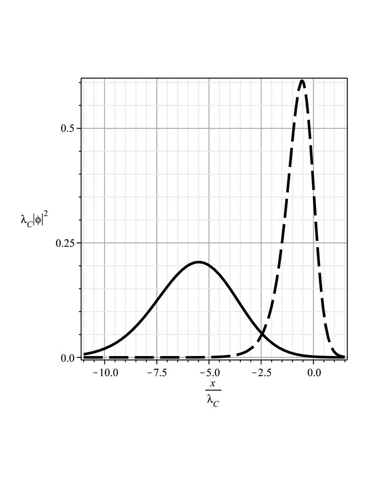
Figure 1: Position probability density for the isolated solution with $v_{0}/mc^{2}=2$ and $\theta=3\pi/8$. The continuous line for $\hbar\gamma/mc=1/10$, and the dashed line for $\hbar\gamma/mc=1$. $\lambda_{C}=\hbar/mc$ denotes the Compton wavelength of the fermion.

one recovers the value for $\phi$ in the case of the sign potential (at large $\gamma$) as in Ref. [11]. Figure 1 illustrates the position probability density for a massive fermion with $v_{0}/mc^{2}=2$, $\theta=3\pi/8$ and two different values of $\gamma$. From this figure one sees that $|\phi|^{2}$ shrinks with rising $\gamma$.

The expectation value of $x$ and $x^{2}$ is given by

$$<x>=-\frac{4\gamma}{2^{2\alpha_{2}}B\left(\alpha_{+},\alpha_{-}\right)}\int_{0}^{\infty}dx\,\frac{x\sinh 2\alpha_{1}x}{\cosh^{2\alpha_{2}}\gamma x}$$ (29)

and

$$<x^{2}>=\frac{4\gamma}{2^{2\alpha_{2}}B\left(\alpha_{+},\alpha_{-}\right)}\int_{0}^{\infty}dx\,\frac{x^{2}\cosh 2\alpha_{1}x}{\cosh^{2\alpha_{2}}\gamma x}$$ (30)

From (A7a) and (A7b) these last results can be simplified to

$$<x>=-\frac{1}{2\gamma}{\Delta}\left(\alpha\right)$$ (31)

and

$$<x^{2}>=\frac{1}{\left(2\gamma\right)^{2}}\,{\Sigma}^{\left(1\right)}\left(\alpha\right)+<x>^{2}$$ (32)

and hence the fermion is confined within an interval $\Delta x=\sqrt{<x^{2}>-<x>^{2}}$ given by

$$\Delta x=\frac{1}{2\gamma}\sqrt{{\Sigma}^{\left(1\right)}\left(\alpha\right)}$$ (33)

Thereby, with the help of (A8b), one obtains the values for $<x>$ and $\Delta x$ either in the case of $\sin\theta\rightarrow 0$ or in the case of the sign potential (at large $\gamma$) as in Ref. [11]:

$$< x>\rightarrow-\text{sgn}\left(v_{0}\right)\frac{\hbar c}{\sin\theta}\frac{mc^{2}}{v_{0}^{2}-m^{2}c^{4}}$$ (34a)

$$\Delta x \rightarrow \frac{\hbar c}{\sqrt{2}\sin\theta}\frac{\sqrt{v_{0}^{2}+m^{2}c^{4}}}{v_{0}^{2}-m^{2}c^{4}}$$ (34b)

On the other hand, from (A9) one sees that when $$\gamma\rightarrow 0 |v_{0}|\rightarrow\infty$$ or

$$< x>\rightarrow\frac{1}{2\gamma}\ln\frac{|v_{0}|-\text{sgn}\left(v_{0}\right)mc^{2}}{|v_{0}|+\text{sgn}\left(v_{0}\right)mc^{2}}$$ (35a)

$$\Delta x \rightarrow \sqrt{\frac{\hbar c}{2\gamma\sin\theta}\frac{|v_{0}|}{v_{0}^{2}-m^{2}c^{4}}}$$ (35b)

Again one can see that the fermion becomes delocalized as $$\sin\theta <x>\rightarrow-\infty \Delta x\rightarrow\infty |v_{0}|\rightarrow mc^{2} <x>\rightarrow 0 \Delta x\rightarrow 0 |v_{0}|\rightarrow\infty$$ decreases and that the best localization occurs for a pure scalar coupling. More than this, and as , and besides and as .

If $\Delta x$ reduces its extension (with rising $|v_{0}|$ or $\sin\theta$ or $\gamma$) then $\Delta p$ must expand, in consonance with the Heisenberg uncertainty principle. Nevertheless, the maximum uncertainty in the momentum is comparable with $mc$ requiring that is impossible to localize a fermion in a region of space less than or comparable with half of its Compton wavelength (see, for example, [22]). This impasse can be broken by resorting to the concepts of effective mass and effective Compton wavelength. Indeed, if one defines an effective mass as $m_{\mathtt{eff}}=m\sqrt{1+\left(v_{0}/mc^{2}\right)^{2}}$ and an effective Compton wavelength $\lambda_{\mathtt{eff}}=\hbar/\left(m_{\mathtt{eff}}c\right)$, one will find

$$\Delta x=\frac{\sqrt{2}\lambda_{\mathtt{eff}}}{4\sin\theta}\sqrt{\left(\alpha_{+}^{2}+\alpha_{-}^{2}\right){\Sigma}^{\left(1\right)}\left(\alpha\right)}$$ (36)

It follows that the high localization of fermions, related to high values of $|v_{0}|$ and $\gamma$, never menaces the single-particle interpretation of the Dirac theory even if the fermion is massless ($m_{\mathtt{eff}}=|v_{0}|/c^{2}$). This fact is convincing because the scalar coupling exceeds the vector coupling, and so the conditions for Klein’s paradox are never reached. As a matter of fact, (34b) furnishes $\left(\Delta x\right)_{\min}\simeq\lambda_{\mathtt{eff}}/(\sqrt{2}\sin\theta)$ for $|v_{0}|\gg mc^{2}$ and $\hbar\gamma\gg mc$.

3.2 The case $E\neq-mc^{2}\cos\theta$

For our model, recalling (14) and (17), one finds

$$\phi_{-}=\frac{-i}{E+mc^{2}\cos\theta}\left[\hbar c\frac{d\phi_{+}}{dx}\,+\left(mc^{2}+v_{0}\,\tanh\gamma x\right)\sin\theta\,\phi_{+}\right]$$ (37)

and

$$V_{\mathtt{eff}}=-V_{1}\text{{sech}}^{2}\gamma x+V_{2}\tanh\gamma x+V_{3}$$ (38)

where the following abbreviations have been used:

$$V_{1} = v_{0}\sin\theta\,\frac{v_{0}\sin\theta+\hbar c\gamma}{2c^{2}}$$ (39a)

$$V_{2} = v_{0}\,\frac{E\cos\theta+mc^{2}}{c^{2}}$$ (39b)

$$V_{3} = \frac{v_{0}^{2}\sin^{2}\theta}{2c^{2}}$$ (39c)

It is instructive to note that if we let $$\gamma\rightarrow\infty \tanh\gamma x\rightarrow \left(x\right) \left(\gamma/2\right) {}^{2}\gamma x\rightarrow\delta\left(x\right) \sin\theta=0 V_{2}>0 V_{2}<0 \sin\theta\neq 0 V_{3}\pm V_{2} x\rightarrow\pm\infty |V_{2}|<2|V_{1}|$$, then sgn and sech. For , the “effective potential” is an ascendant (a descendant) smooth step if (). For , though, the “effective potential” has the same form as the exactly solvable Rosen-Morse potential [16], [23]. The Rosen-Morse potential approaches as and has an extremum when at

$$x_{m}=\frac{1}{2\gamma}\ln\left(\frac{2V_{1}-V_{2}}{2V_{1}+V_{2}}\right)$$ (40)

As a matter of fact, potential-well structures can be achieved when $|V_{2}|<2|V_{1}|$   with $V_{1}>0$. To acknowledge that the effective potential for the mixing given by (9) is a Rosen-Morse potential can help you to see more clearly how a kink-like smooth step potential might furnish a finite set of bound-state solutions. After all, we shall not use the knowledge about the exact analytical solution for the Rosen-Morse potential.

3.2.1 The asymptotic solutions

As $|x|\gg 1/\gamma$ the effective potential is practically constant (the main transition region occurs in $|x|<1/\gamma$) and the solutions for the Dirac equation can be approximate by those ones for a free particle. Furthermore, the asymptotic behaviour will show itself suitable to impose the appropriate boundary conditions to the complete solution to the problem.

We turn our attention to scattering states for fermions coming from the left. Then, $\phi$ for $x\rightarrow-\infty$ describes an incident wave moving to the right and a reflected wave moving to the left, and $\phi$ for $x\rightarrow+\infty$ describes a transmitted wave moving to the right or an evanescent wave. The upper components for scattering states are written as

$$\phi_{+}=\left\{\begin{array}[]{cc}A_{+}e^{+ik_{-}x}+A_{-}e^{-ik_{-}x},&\text{for\quad}x\rightarrow-\infty\\ &\\ B_{\pm}e^{\pm ik_{+}x},&\text{for\quad}x\rightarrow+\infty\end{array}\right.$$ (41)

where

$$\hbar k_{\pm}=\sqrt{2\left(E_{\mathtt{eff}}-V_{3}\mp V_{2}\right)}$$ (42)

Note that $k_{+}$ is a real number for a progressive wave and an imaginary number for an evanescent wave ($k_{-}$ is a real number for scattering states). Therefore,

$$J^{1}\left(-\infty\right)=\frac{2\hbar c^{2}k_{-}}{E+mc^{2}\cos\theta}\left(|A_{\pm}|^{2}-|A_{\mp}|^{2}\right),\text{\quad for\quad}E\gtrless-mc^{2}\cos\theta$$ (43)

and

$$J^{1}\left(+\infty\right)=\pm\,\frac{2\hbar c^{2}\text{Re}\,k_{+}}{E+mc^{2}\cos\theta}\,|B_{\pm}|^{2},\text{\quad for\quad}E\gtrless-mc^{2}\cos\theta$$ (44)

Note that $J^{1}\left(-\infty\right)=J_{\mathtt{inc}}-J_{\mathtt{ref}}$ and $J^{1}\left(+\infty\right)=J_{\mathtt{tran}}$, where $J_{\mathtt{inc}}$, $J_{\mathtt{ref}}$ and $J_{\mathtt{tran}}$ are nonnegative quantities characterizing the incident, reflected and transmitted waves, respectively. Note also that the roles of $A_{+}$ and $A_{-}$ are exchanged as the sign of $E+mc^{2}\cos\theta$ changes. In fact, if $E>-mc^{2}\cos\theta$, then $A_{+}e^{+ik_{-}x}$ ($A_{-}e^{-ik_{-}x}$) will describe the incident (reflected) wave, and $B_{-}=0$. On the other hand, if $E<-mc^{2}\cos\theta$, then $A_{-}e^{-ik_{-}x}$ ($A_{+}e^{+ik_{-}x}$) will describe the incident (reflected) wave, and $B_{+}=0$. Therefore, the reflection and transmission amplitudes are given by

$$r=\frac{A_{\mp}}{A_{\pm}},\text{\quad}t=\frac{B_{\pm}}{A_{\pm}},\text{\quad for\quad}E\gtrless-mc^{2}\cos\theta$$ (45)

To determine the transmission coefficient we use the current densities $J^{1}\left(-\infty\right)$ and $J^{1}\left(+\infty\right)$. The $x$-independent space component of the current allows us to define the reflection and transmission coefficients as

$$R=\frac{|A_{\mp}|^{2}}{|A_{\pm}|^{2}},\text{\quad}T=\frac{\text{Re}\,k_{+}}{k_{-}}\frac{|B_{\pm}|^{2}}{|A_{\pm}|^{2}},\text{\quad for\quad}E\gtrless-mc^{2}\cos\theta$$ (46)

Notice that $R+T=1$ by construction.

3.2.2 The complete solutions

Armed with the knowledge about asymptotic solutions and with the definition of the transmission coefficient we proceed for searching solutions on the entire region of space.

Changing the independent variable $x$ in (16) to

$$y=\frac{1}{2}\left(1-\tanh\gamma x\right)$$ (47)

the differential equation is transformed into

$$y\left(1-y\right)\frac{d^{2}\phi_{+}}{dy^{2}}+\left(1-2y\right)\frac{d\phi_{+}}{dy}+\Theta\phi_{+}=0$$ (48)

where

$$\Theta=\frac{4V_{1}y\left(1-y\right)-V_{2}\left(1-2y\right)-V_{3}+E_{\mathtt{eff}}}{2\left(\hbar\gamma\right)^{2}y\left(1-y\right)}$$ (49)

regardless of the sign of $x$. Introducing a new function $\varphi(y)$ through the relation

$$\phi_{+}(y)=y^{\nu}\left(1-y\right)^{\mu}\varphi(y)$$ (50)

and defining

$$a = \mu+\nu+\frac{1-\omega}{2},\quad b=\mu+\nu+\frac{1+\omega}{2},\quad d=2\nu+1$$ (51a)

$$\mu^{2} = -\left(\frac{k_{-}}{2\gamma}\right)^{2},\quad\nu^{2}=-\left(\frac{k_{+}}{2\gamma}\right)^{2},\quad\omega^{2}=1+\frac{8V_{1}}{\left(\hbar\gamma\right)^{2}}$$ (51b)

Eq. (48) becomes the hypergeometric differential equation [24]

$$y\left(1-y\right)\frac{d^{2}\varphi}{dy^{2}}+\left[d-\left(a+b+1\right)y\right]\frac{d\varphi}{dy}-ab\varphi=0$$ (52)

whose general solution can be written in terms of the Gauss hypergeometric series

$${}_{2}F_{1}\left(a,b,d,y\right)=\frac{\Gamma\left(d\right)}{\Gamma\left(a\right)\Gamma\left(b\right)}\sum\limits_{n=0}^{\infty}\frac{\Gamma\left(a+n\right)\Gamma\left(b+n\right)}{\Gamma\left(d+n\right)}\frac{y^{n}}{n!}$$ (53)

in the form [24]

$$\varphi=A\;_{2}F_{1}\left(a,b,d,y\right)+By^{-2\nu}\;_{2}F_{1}\left(a+1-d,b+1-d,2-d,y\right)$$ (54)

in such a way that

$$\phi_{+}=A\,y^{\nu}\left(1-y\right)^{\mu}\;_{2}F_{1}\left(a,b,d,y\right)$$

$$+\,B\,y^{-\nu}\left(1-y\right)^{\mu}\;_{2}F_{1}\left(a+1-d,b+1-d,2-d,y\right)$$ (55)

with the constants $A$ and $B$ to be fitted by the asymptotic behaviour analyzed in the previous discussion.

As $x\rightarrow+\infty$ (that is, as $y\rightarrow 0$), one has that $y\simeq\exp\left(-2\gamma x\right)$ and (55), because ${}_{2}F_{1}\left(a,b,d,0\right)=1$, reduces to

$$\phi_{+}\left(+\infty\right)\simeq Ae^{-2\gamma\nu x}+Be^{2\gamma\nu x}$$ (56)

so the asymptotic behaviour, for $\nu=\mp ik_{+}/\left(2\gamma\right)$, requires that $B=0$ and $A=B_{\pm}$ corresponding to $E\gtrless-mc^{2}\cos\theta$, or equivalently $A=0$ and $B=B_{\mp}$ corresponding to $E\lessgtr-mc^{2}\cos\theta$. We choose $B=0$.

The asymptotic behaviour as $x\rightarrow-\infty$ ($y\rightarrow 1$) can be found by using the relation for passing over from $y$ to $1-y$:

$${}_{2}F_{1}\left(a,b,d,y\right)=\gamma_{-}\;{}_{2}F_{1}\left(a,b,a+b-d+1,1-y\right)$$

$$+\,\,\gamma_{+}\;{}_{2}F_{1}\left(d-a,d-b,d-a-b+1,1-y\right)\left(1-y\right)^{d-a-b}$$ (57)

where $\gamma_{+}$ and $\gamma_{-}$ are expressed in terms of the gamma function as

$$\gamma_{-}=\frac{\Gamma\left(d\right)\Gamma\left(d-a-b\right)}{\Gamma\left(d-a\right)\Gamma\left(d-b\right)},\quad\gamma_{+}=\frac{\Gamma\left(d\right)\Gamma\left(a+b-d\right)}{\Gamma\left(a\right)\Gamma\left(b\right)}\quad$$ (58)

which can also be written as

$$\gamma_{\pm}=\frac{\Gamma\left(2\nu+1\right)\Gamma\left(\pm 2\mu\right)}{\Gamma\left(\frac{1+\omega}{2}+\nu\pm\mu\right)\Gamma\left(\frac{1-\omega}{2}+\nu\pm\mu\right)}$$ (59)

Now, as $x\rightarrow-\infty$, $1-y\simeq\exp\left(+2\gamma x\right)$. This time, (55) tends to

$$\phi_{+}\left(-\infty\right)\simeq A\gamma_{+}e^{-2\gamma\mu x}+A\gamma_{-}e^{+2\gamma\mu x}$$ (60)

so that $A\gamma_{+}=A_{\pm}$ and $A\gamma_{-}=A_{\mp}$ for $\mu=\mp ik_{-}/\left(2\gamma\right)$, in accordance with the previous analysis for very large negative values of $x$.

Those asymptotic behaviours are all one needs to determinate the transmission amplitude (45) and the transmission coefficient (46). Now, these quantities can now be expressed in terms of $\gamma_{\pm}$ as

$$\text{\quad}t=\frac{1}{\gamma_{\pm}},\text{\quad}T=\left|\frac{\text{Im}\nu}{\mu}\right|\frac{1}{|\gamma_{\pm}|^{2}},\text{\quad for\quad}\mu=\mp\frac{ik_{-}}{2\gamma}$$ (61)

Notice that $\omega^{2}$ in (51b) can be written as

$$\omega^{2}=\left(1+\frac{2v_{0}\sin\theta}{\hbar c\gamma}\right)^{2}$$ (62)

so that

$$\omega=\pm\left(1+\frac{2v_{0}\sin\theta}{\hbar c\gamma}\right)$$ (63)

Furthermore, by using the following identities [24]

$$|\Gamma\left(iv\right)|^{2}=\frac{\pi}{v\sinh\pi v},\quad|\Gamma\left(1+iv\right)|^{2}=\frac{\pi v}{\sinh\pi v}$$ (64)

added by the identity [14]

$$|\Gamma\left(u+iv\right)\Gamma\left(1-u+iv\right)|^{2}=\frac{2\pi^{2}}{\cosh 2\pi v-\cos 2\pi u}$$ (65)

where $u$ and $v$ are the real and imaginary parts of a complex number, one can show that

$$T=\frac{2\sinh\frac{k_{-}\pi}{\gamma}\sinh\text{Re}\,\frac{k_{+}\pi}{\gamma}}{\left|\cosh\frac{\left(k_{-}+k_{+}\right)\pi}{\gamma}+\cos\pi\omega\right|}$$ (66)

taking no regard if $E>-mc^{2}\cos\theta$ or $E<-mc^{2}\cos\theta$. Nevertheless, scattering states are possible only if $|E+v_{0}\cos\theta|>|mc^{2}-v_{0}|$ because $k_{-}$ is a real number, and there is a transmitted wave only if $|E-v_{0}\cos\theta|>|mc^{2}+v_{0}|$. As $|E|\rightarrow\infty$, $T\rightarrow 1$ as it should be. Seen as a function of $E$, for $E>-mc^{2}\cos\theta$, the transmission coefficient presents a profile typical for the nonrelativistic scattering in a step potential. Seen as a function of the mixing angle the transmission coefficient presents some intriguing results explained by observing that the effective potential presents an ascendant (descendant) step for small (large) values of $\theta$ (see Ref. [11] for $\gamma\rightarrow\infty$). The transmission coefficient vanishes for enough small mixing angles and energies because the effective energy is smaller than the height of the effective step potential. For $|v_{0}|>mc^{2}$, the absence of scattering for enough large mixing angles and enough small energies occurs because the effective energy is smaller than the effective step potential in the region of incidence.

By the way, as $\gamma\rightarrow 0$ one finds

$$T=\left\{\begin{array}[]{cc}1,&\text{for\quad}k_{+}\in\mathbb{R}\\ &\\ 0,&\text{for\quad}k_{+}=\pm i|k_{+}|\end{array}\right.$$ (67)

reflecting our expectation about the absence of quantum effects for a potential whose interval of appreciable variation is much more larger than the Compton wavelength. It is remarkable that this “classical” scattering also takes place for massless fermions. On the other hand, for $\gamma\rightarrow\infty$ one finds the transmission coefficient for the sign step potential [11]:

$$T\simeq\frac{4k_{-}\text{Re}\,k_{+}}{\left(k_{-}+k_{+}\right)^{2}+\left(\frac{2v_{0}\sin\theta}{{}_{\hbar c}}\right)^{2}}$$ (68)

as it should be.

3.2.3 Bound states

The possibility of bound states requires a solution with an asymptotic behaviour given by (41) with $k_{\pm}=i|k_{\pm}|$ and $A_{+}=B_{-}=0$, or $k_{\pm}=-i|k_{\pm}|$ and $A_{-}=B_{+}=0$, to obtain a square-integrable $\phi_{+}$, meaning that

$$E_{\mathtt{eff}}<V_{3}\pm V_{2}$$ (69)

or equivalently

$$|E\pm v_{0}\cos\theta|<|mc^{2}\mp v_{0}|$$ (70)

On the other hand, if one considers the transmission amplitude $t$ in (61) as a function of the complex variables $k_{\pm}$ one sees that for $k_{\pm}>0$ ($\mu$ and $\nu$ as imaginary quantities) one obtains the scattering states whereas the bound states would be obtained by the poles lying along the imaginary axis of the complex $k$-plane. From (56) with $B=0$ one sees that $\nu$ is a positive quantity. On the other hand, $\mu$ is positive (negative) if $\gamma_{+}=0$ ($\gamma_{-}=0$). The poles of the transmission amplitude are given by the zeros of $\gamma_{\pm}$. It happens that $\Gamma\left(z\right)$ has no zeros but it has simple poles on the real axis at $z=-n$ with $n=0,1,2,\ldots$ Because ${}_{2}F_{1}\left(a,b,d,y\right)$ is invariant under exchange of $a$ and $b$, the quantization condition is thus given by $a=-n$ or $b=-n$. Therefore, the bound states occur only for

$$|\mu|+|\nu|+\frac{1-|\omega|}{2}=-n$$ (71)

Recalling the definitions of $\mu$, $\nu$ and $\omega$ given in (51), the quantization condition can be rewritten as

$$\sqrt{\left(mc^{2}+v_{0}\right)^{2}-\left(E-v_{0}\cos\theta\right)^{2}}+\sqrt{\left(mc^{2}-v_{0}\right)^{2}-\left(E+v_{0}\cos\theta\right)^{2}}$$

$$=2\hbar c\gamma\left(\pm\frac{v_{0}\sin\theta}{\hbar c\gamma}-N\right),\text{\quad for\quad}\frac{v_{0}\sin\theta}{\hbar c\gamma}\gtrless-\frac{1}{2}$$ (72)

with

$$N=\left\{\begin{array}[]{c}n,\\ \\ n+1,\end{array}\begin{array}[]{c}\text{\quad for\quad}\frac{v_{0}\sin\theta}{\hbar c\gamma}>-\frac{1}{2}\\ \\ \text{\quad for\quad}\frac{v_{0}\sin\theta}{\hbar c\gamma}<-\frac{1}{2}\end{array}\right.$$ (73)

Because the first line of (72) is a positive number and $n$ is a nonnegative integer, one finds supplementary restrictions imposed on $v_{0}\sin\theta/\left(\hbar c\gamma\right)$ and $N$:

$$\frac{v_{0}\sin\theta}{\hbar c\gamma}>0,\text{\quad}N<\frac{v_{0}\sin\theta}{\hbar c\gamma}$$ (74)

or

$$\frac{v_{0}\sin\theta}{\hbar c\gamma}<-1,\text{\quad}N<-\frac{v_{0}\sin\theta}{\hbar c\gamma}$$ (75)

This means that there is a finite set of bound-state solutions depending on the sign and size of $v_{0}\sin\theta/\left(\hbar c\gamma\right)$, and that the number of allowed solutions increases with $|v_{0}|\sin\theta/\left(\hbar c\gamma\right)$. It is worth to mention that the threshold ($|v_{0}|_{\min}$) is an increasing monotonic function of $\gamma$ with $|v_{0}|_{\min}\rightarrow mc^{2}$ as $\gamma\rightarrow 0$ so that the existence of those bound-state solutions is not workable in a nonrelativistic scheme. In particular, there is no bound-state solution neither when $\sin\theta=0$ nor in the limiting case $\gamma\rightarrow\infty$. Furthermore, the symmetries related to the charge-conjugation and chiral-conjugation operations discussed in Sec. 2 are clearly revealed. It is interesting to remark that the conditions on $v_{0}\sin\theta/\left(\hbar c\gamma\right)$ in (74) and (75) are these ones that make $V_{1}>0$ in (39a).

The irrational equation (72) can be solved iteratively to determine the eigenenergies. However, if one squares (72), the resulting quantization condition can also be expressed as a second-order algebraic equation in $E$ with two branches of solutions

$$E=\frac{-c_{1}\pm\sqrt{c_{1}^{2}-4c_{2}c_{0}}}{2c_{2}}$$ (76)

where

$$c_{2} = v_{0}^{2}+(\hbar c\gamma N)^{2}-2\left(\hbar c\gamma N\right)|v_{0}|\sin\theta$$ (77a)

$$c_{1} = 2mc^{2}v_{0}^{2}\cos\theta$$ (77b)

$$c_{0} = (\hbar c\gamma N)^{4}-4(\hbar c\gamma N)^{3}|v_{0}|\sin\theta+(\hbar c\gamma N)^{2}\left(5v_{0}^{2}\sin^{2}\theta-m^{2}c^{4}\right)$$ (77c)

$$+2(\hbar c\gamma N)\left(m^{2}c^{4}-v_{0}^{2}\sin^{2}\theta\right)|v_{0}|\sin\theta+m^{2}c^{4}v_{0}^{2}\cos^{2}\theta$$

The price paid by those analytical solutions is that some of them can be spurious. Of course, the false roots can be eliminated by inspecting whether they satisfy the original equation. Furthermore, despite the closed form for the Dirac eigenenergies, the solutions given by (76) present an intricate dependence on $$|v_{0}| \gamma \theta m N n=0 v_{0}>0 n=0 v_{0}>0 E=-mc^{2}\cos\theta v_{0}<0 v_{0}>0 |v_{0}|\sin\theta/\left(\hbar c\gamma\right) |v_{0}|\sin\theta/\left(\hbar c\gamma\right)+1 n n-1$$, , , and . There is an evident problem with the solution when because Eq. (76) with and presents the unique root . This, of course, is not a proper solution of the problem. The results for are the same as those ones for if one changes by and by .

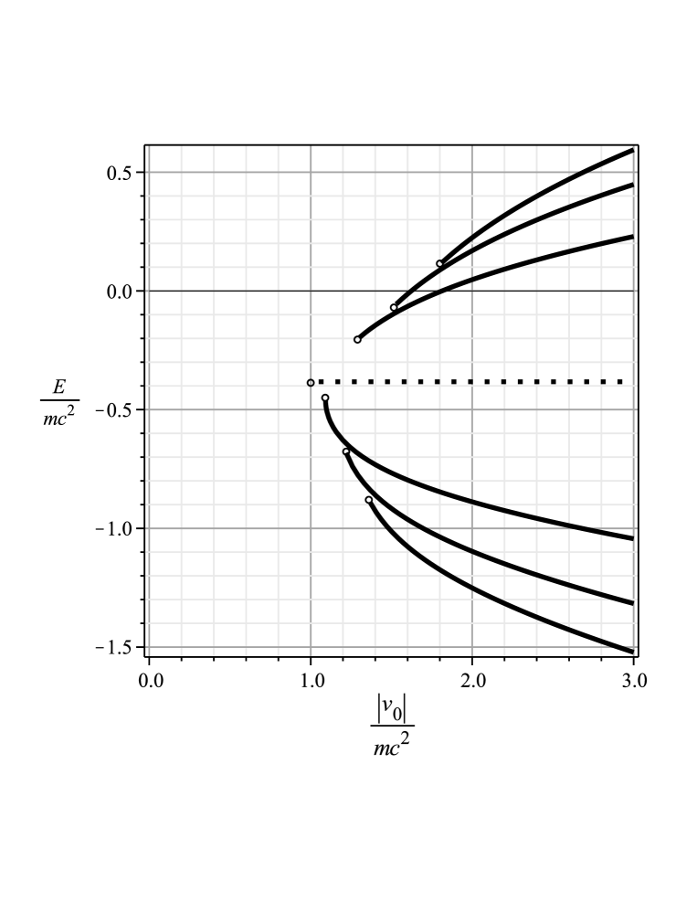
Figure 2: Energy levels for the three lowest quantum numbers ($n=1,2,3$ for $v_{0}>0$) with $\theta=3\pi/8$ and $\hbar\gamma/mc=1/10$. The innermost curves are related to the lowest quantum numbers. The dotted line is related to the isolated solution.

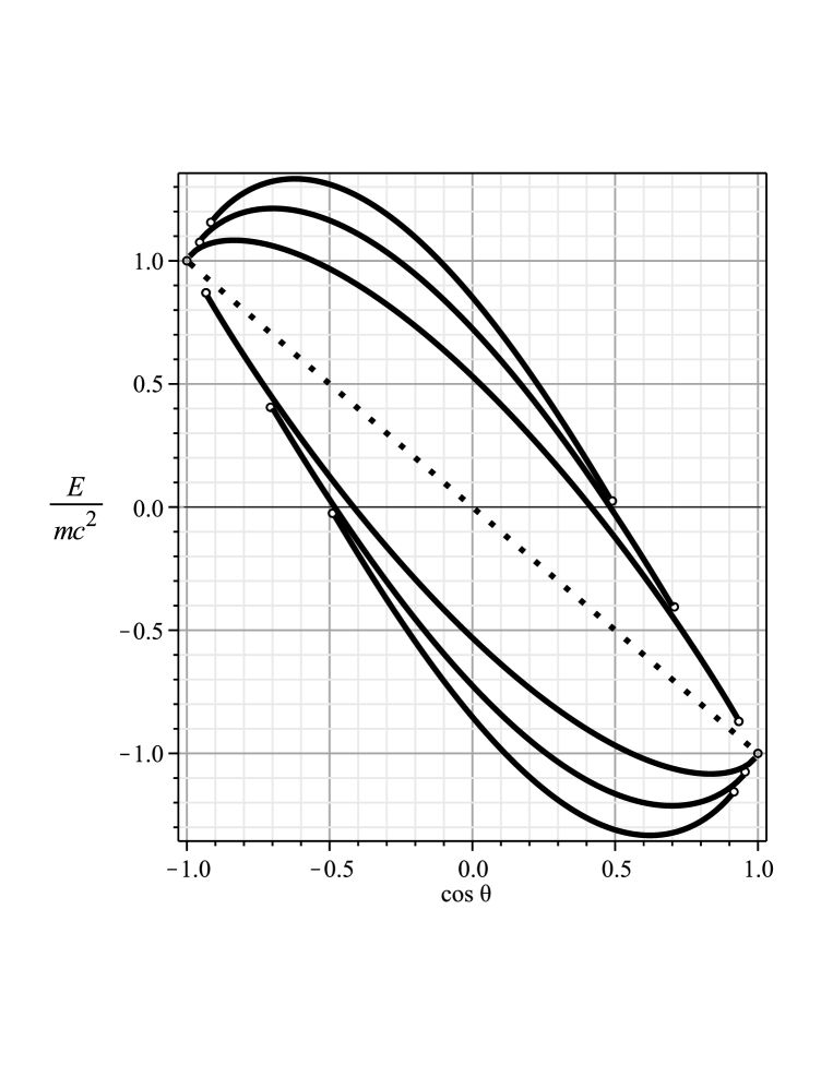
Figure 3: The same as Figure 2, for $v_{0}/mc^{2}=2$ and $\hbar\gamma/mc=1/10$.

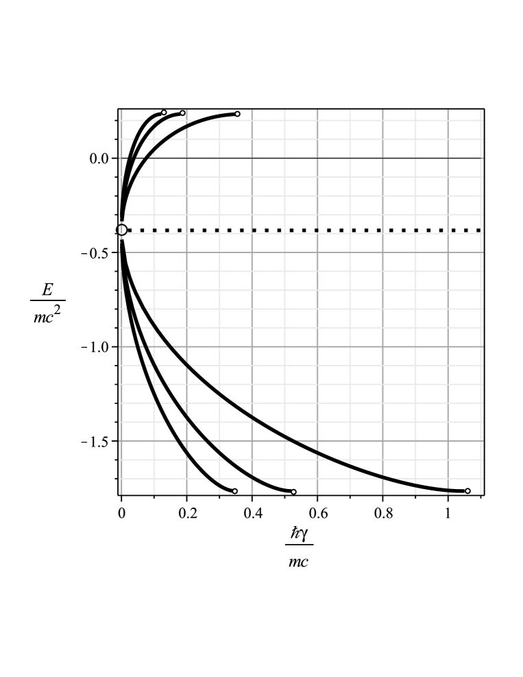
Figure 4: The same as Figure 2, for $\theta=3\pi/8$ and $v_{0}/mc^{2}=2$.

Numerical solutions for the eigenenergies corresponding to the three lowest quantum numbers ($n=1,2,3$ for $v_{0}>0$) are shown in Figures 2, 3 and 4 for a massive fermion. In all of these figures, the innermost curves correspond to the lowest quantum numbers and the dotted line corresponds to the isolated solution ($E=-mc^{2}\cos\theta$) discussed in the previous section.

In Fig. 2 we show the eigenenergies as a function of $|v_{0}|/mc^{2}$ for $\theta=3\pi/8$ and $\hbar\gamma/mc=1/10$. Notice that a minimum value for $|v_{0}|$ is required to obtain at least one energy level and that because $\theta<\pi/2$ the branch of solutions with $E<-mc^{2}\cos\theta$ is more favoured. Notice also that more and more energy levels arise for each branch as $v_{0}$ increases.

In Fig. 3 the eigenenergies are shown as a function of $\cos\theta$ for $v_{0}/mc^{2}=2$ and $\hbar\gamma/mc=1/10$. It is remarkable that the eigenenergy changes from $E$ to $-E$ when $\theta$ changes from $\pi/2-\varepsilon$ to $\pi/2+\varepsilon$. In particular, the energy levels exhibit symmetry about $E=0$ when $\theta=\pi/2$. All of the levels tend to vanish as $\cos\theta$ tends to $\pm 1$. Incidentally, this disappearance of energy levels is more forceful for higher values of $n$. The branch for $E\gtrless-mc^{2}\cos\theta$ is more favored when $\theta\lessgtr\pi/2$.

In Fig. 4 the eigenenergies are shown as a function of $\hbar\gamma/mc$ for $\theta=3\pi/8$ and $v_{0}/mc^{2}=2$. For $\gamma\simeq 0$ we have a very high density of energy levels. These levels correspond to very delocalized states due to the large extension of the interaction region. The density of energy levels decreases with increasing $\hbar\gamma/mc$. It is worth noting that the energy levels exist in a finite interval of $\hbar\gamma/mc$, and so they do not exist in the extreme relativistic regime for a finite value of $|v_{0}|/mc^{2}$. It should be mentioned, though, the upper limit of $\hbar\gamma/mc$ increases monotonously with $|v_{0}|/mc^{2}$. Notice also that because $\theta<\pi/2$ the branch of solutions with $E<-mc^{2}\cos\theta$ is more favoured.

The case of a massless fermion, as already discussed before with fulcrum on the charge-conjugation and the chiral-conjugation operations, presents a spectrum symmetrical about $E=0$ and seen as a function of $\theta$ exhibits an additional symmetry about $\theta=\pi/2$.

Now the Gauss hypergeometric series ${}_{2}F_{1}\left(a,b,d,y\right)$ reduces to nothing but a polynomial of degree $n$ in $y$ when $a$ or $b$ is equal to $-n$: Jacobi’s polynomial of index $\alpha$ and $\beta$. Indeed, for $a=-n$ one has [24]

$${}_{2}F_{1}\left(a,b,d,y\right) = {}_{2}F_{1}\left(-n,\alpha+1+\beta+n,\alpha+1,y\right)$$ (78)

$$= \frac{n!}{\left(\alpha+1\right)_{n}}P_{n}^{\left(\alpha,\beta\right)}\left(\xi\right)$$

where

$$\alpha=2|\nu|,\quad\beta=2|\mu|,\quad\xi=1-2y$$ (79)

and $\left(\alpha\right)_{n}=\alpha\left(\alpha+1\right)\left(\alpha+2\right)...\left(\alpha+n-1\right)$ with $\left(\alpha\right)_{0}=1$. Hence $\phi_{+}$ can be written as

$$\phi_{+}\left(\xi\right)=N_{n}\left(1-\xi\right)^{\alpha/2}\left(1+\xi\right)^{\beta/2}P_{n}^{\left(\alpha,\beta\right)}\left(\xi\right)$$ (80)

and $\phi_{-}$ assumes the form

$$\phi_{-}\left(\xi\right)=\frac{-i\hbar c\gamma}{E+mc^{2}\cos\theta}\left[\left(1-\xi^{2}\right)\frac{d\phi_{+}}{d\xi}+\frac{mc^{2}+v_{0}\xi}{\hbar c\gamma}\sin\theta\,\phi_{+}\right]$$ (81)

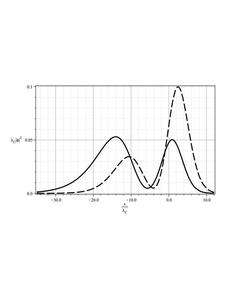
Figure 5: Position probability density for the Sturm-Liouville solution with $n=1$, $v_{0}/mc^{2}=2$, $\hbar\gamma/mc=1/10$ and $\theta=3\pi/8$. The continuous line for $E/mc^{2}=+0.047$, and the dashed line for $E/mc^{2}=-0.888$. $\lambda_{C}=\hbar/mc$ denotes the Compton wavelength of the fermion.

Because Jacobi’s polynomials $P_{n}^{\left(\alpha,\beta\right)}\left(\xi\right)$ have $n$ distinct zeros [24] $\phi_{+}$ has $n$ nodes, and this fact causes $|\phi|^{2}$ to have between $n+1$ and $2n+1$ humps. The position probability density has a lonely hump exclusively for the isolated solution. The determination of the normalization constant $N_{n}$ looks exceedingly complicated and so we content ourselves with a numerical illustration. Figure 5 shows the normalized position probability density for a massive fermion for the Sturm-Liouville solution with $n=1$, $v_{0}/mc^{2}=2$, $\hbar\gamma/mc=1/10$ and $\theta=3\pi/8$.

4 Final remarks

We have assessed the stationary states of a fermion under the influence of the kink-like potential $\tanh\gamma x$ as a generalization of the sign potential (see [11]). Several interesting properties arose depending on the size of the skew parameter $\gamma$. For a special mixing of scalar and vector couplings, a continuous chiral-conjugation transformation was allowed to decouple the upper and lower components of the Dirac spinor and to assess the scattering problem under a Sturm-Liouville perspective. A finite set of intrinsically relativistic bound-state solutions was computed directly from the poles of the transmission amplitude. An isolated solution from the Sturm-Liouville problem corresponding to a bound state was also analyzed. The concepts of effective mass and effective Compton wavelength were used to show the impossibility of pair production under a strong potential despite the high localization of the fermion. It was also shown that all of the bound-state solutions disappear asymptotically as one approaches the conditions for the realization of “spin and pseudospin symmetries”.

Appendix A Useful integrals and limits

The integral necessary for calculating the normalization constants in (21) and (22) is tabulated (see the formula 3.512.1, or 8.380.10, in Ref. [25]):

$$\int_{0}^{\infty}dx\,\frac{\cosh 2\beta_{1}x}{\cosh^{2\beta_{2}}\gamma x}=\frac{2^{2\beta_{2}}}{4\gamma}B\left(\beta_{2}+\frac{\beta_{1}}{\gamma},\beta_{2}-\frac{\beta_{1}}{\gamma}\right)$$ (A1)

where

$$B\left(z_{1},z_{2}\right)=\frac{\Gamma\left(z_{1}\right)\Gamma\left(z_{2}\right)}{\Gamma\left(z_{1}+z_{2}\right)},\text{\quad Re\thinspace}z_{1}>0,\text{\quad Re\thinspace}z_{2}>0$$ (A2)

is the beta function [24].

We now proceed to evaluate the integrals in (29) and (30). We introduce an accessory parameter $\lambda$ in such a way that

$$\int_{0}^{\infty}dx\,\frac{x\sinh 2\lambda\beta_{1}x}{\cosh^{2\beta_{2}}\gamma x}=\frac{1}{2\beta_{1}}\frac{\partial I\left(\lambda\right)}{\partial\lambda}$$ (A3a)

$$\int_{0}^{\infty}dx\,\frac{x^{2}\cosh 2\lambda\beta_{1}x}{\cosh^{2\beta_{2}}\gamma x}=\frac{1}{4\beta_{1}^{2}}\frac{\partial^{2}I\left(\lambda\right)}{\partial\lambda^{2}}$$ (A3b)

where

$$I\left(\lambda\right)=\int_{0}^{\infty}dx\,\frac{\cosh 2\lambda\beta_{1}x}{\cosh^{2\beta_{2}}\gamma x}=\frac{2^{2\beta_{2}}}{4\gamma}B\left(\beta_{+},\beta_{-}\right)$$ (A4)

and $\beta_{\pm}\left(\lambda\right)=\beta_{2}\pm\lambda\beta_{1}/\gamma$. Defining

$${\Delta}\left(\beta\right)=\boldsymbol{\psi\,}\left(\beta_{+}\right)-\boldsymbol{\psi\,}\left(\beta_{-}\right),\quad{\Sigma}^{\left(1\right)}\left(\beta\right)=\boldsymbol{\psi\,}^{\left(1\right)}\left(\beta_{+}\right)+\boldsymbol{\psi\,}^{\left(1\right)}\left(\beta_{-}\right)$$ (A5)

where $\boldsymbol{\psi\,}\left(z\right)=d\ln\Gamma\left(z\right)/dz$ is the digamma (psi) function and $\boldsymbol{\psi\,}^{\left(1\right)}\left(z\right)=d\boldsymbol{\psi\,}\left(z\right)/dz$ is the trigamma function [24], printed in a boldface type to differ from the Dirac eigenspinor in Sec. 2, one can write

$$\frac{\partial}{\partial\lambda}B\left(\beta_{+},\beta_{-}\right)=\frac{\beta_{1}}{\gamma}B\left(\beta_{+},\beta_{-}\right){\Delta}\left(\beta\right)$$ (A6a)

$$\frac{\partial^{2}}{\partial\lambda^{2}}B\left(\beta_{+},\beta_{-}\right)=\left(\frac{\beta_{1}}{\gamma}\right)^{2}B\left(\beta_{+},\beta_{-}\right)\left[{\Sigma}^{\left(1\right)}\left(\beta\right)+{\Delta}^{2}\left(\beta\right)\right]$$ (A6b)

Finally, setting the parameter $\lambda=1$ and defining $\widetilde{\beta}_{\pm}=\beta_{\pm}\left(1\right)$, one finds

$$\int_{0}^{\infty}dx\,\frac{x\sinh 2\beta_{1}x}{\cosh^{2\beta_{2}}\gamma x}=\frac{2^{2\beta_{2}}}{8\gamma^{2}}B\left(\widetilde{\beta}_{+},\widetilde{\beta}_{-}\right){\Delta}\left(\widetilde{\beta}\right)$$ (A7a)

$$\int_{0}^{\infty}dx\,\frac{x^{2}\cosh 2\beta_{1}x}{\cosh^{2\beta_{2}}\gamma x}=\frac{2^{2\beta_{2}}}{16\gamma^{3}}B\left(\widetilde{\beta}_{+},\widetilde{\beta}_{-}\right)\left[{\Sigma}^{\left(1\right)}\left(\widetilde{\beta}\right)+{\Delta}^{2}\left(\widetilde{\beta}\right)\right]$$ (A7b)

for Re $\widetilde{\beta}_{\pm}>0$.

Notice that because $\Gamma\left(z\right)$ has simple poles at $z=-n$ with residue $\left(-1\right)^{n}/n!$ [24], one has $\Gamma\left(z\right)\simeq z^{-1}$ for $z\simeq 0$. As a consequence,

$$B\left(z_{1},z_{2}\right)\simeq\frac{1}{z_{1}}+\frac{1}{z_{2}},\text{\quad for\quad}z_{1}\simeq z_{2}\simeq 0$$ (A8a)

and

$$\boldsymbol{\psi\,}\left(z\right)\simeq-\frac{1}{z},\text{\quad}\boldsymbol{\psi\,}^{\left(1\right)}\left(z\right)\simeq\frac{1}{z^{2}},\text{\quad for\quad}z\simeq 0$$ (A8b)

On the other hand, because $\ln\Gamma\left(z\right)\simeq z\ln z$ for $z>>1$ [24], one finds

$$\boldsymbol{\psi\,}\left(z\right)\simeq\ln z,\quad\boldsymbol{\psi\,}^{\left(1\right)}\left(z\right)\simeq\frac{1}{z},\text{\quad for\quad}z>>1$$ (A9)

Acknowledgments

The authors gratefully acknowledge an anonymous referee for his/her valuable comments and suggestions. This work was supported in part by means of funds provided by CNPq.

References

• [1] P.R. Page et al, Phys. Rev. Lett. 86 (2001) 204.
• [2] J.N. Ginocchio, Phys. Rep. 414 (2005) 165.
• [3] J.N. Ginocchio, Phys. Rev. Lett. 78 (1997) 436;
J.N. Ginocchio, A. Leviatan, Phys. Lett. B 425 (1998) 1;
G.A. Lalazissis et al, Phys. Rev. C 58 (1998) R45;
J. Meng et al, Phys. Rev. C 58 (1998) R628;
K. Sugawara-Tanabe, A. Arima, Phys. Rev. C 58 (1998) R3065;
J.N. Ginocchio, Phys. Rep. 315 (1999) 231;
S. Marcos et al, Phys. Rev. C 62 (2000) 054309;
P. Alberto et al, Phys. Rev. Lett. 86 (2001) 5015;
S. Marcos et al, Phys. Lett. B 513 (2001) 36;
J.N. Ginocchio, A. Leviatan, Phys. Rev. Lett. 87 (2001) 072502;
P. Alberto et al, Phys. Rev. C 65 (2002) 034307;
J.N. Ginocchio, Phys. Rev. C 66 (2002) 064312;
T.-S. Chen et al, Chin. Phys. Lett. 20 (2003) 358;
S.-G. Zhou et al, Phys. Rev. Lett. 91 (2003) 262501;
G. Mao, Phys. Rev. C 67 (2003) 044318;
R. Lisboa et al, Phys. Rev. C 69 (2004) 024319;
A. Leviatan, Phys. Rev. Lett. 92 (2004) 202501;
J.-Y. Guo, Phys. Lett. A 338 (2005) 90;
P. Alberto et al, Phys. Rev. C 71 (2005) 034313;
J.-Y. Guo et al, Phys. Rev. C72 (2005) 054319;
J.-Y. Guo et al, Nucl. Phys. A 757 (2005) 411;
C. Berkdemir, Nucl. Phys. A 770 (2006) 32;
Q. Xu, S.-J. Zhu, Nucl. Phys. A 768 (2006) 161;
X.T. He et al, Eur. Phys. J. A 28 (2006) 265;
R.V. Jolos, V.V. Voronov, Phys. Atomic Nuclei 70 (2007) 812;
C.-Y. Song et al, Chin. Phys. Lett. 26 (2009) 122102;
H. Liang et al, Eur. Phys. J. A 44 (2010) 119;
R. Lisboa et al, Phys. Rev. C 81 (2010) 064324;
C.-Y. Song, J.-M. Yao, Chin. Phys. C. 34 (2010) 1425;
H. Liang et al, Phys. Rev. C 83 (2011) 041301(R);
C.-Y. Song et al, Chin. Phys. Lett. 28 (2011) 092101;
B.-N. Lu et al, Phys. Rev. Lett. 109 (2012) 072501;
A.S. de Castro, P. Alberto, Phys. Rev. A 86 (2012) 032122;
P. Alberto et al, Phys. Rev C 87 (2013) 031301(R);
P. Alberto et al, J. Phys.: Conference Series 490 (2014) 012069.
• [4] P. Alberto et al, Phys. Rev. C 75 (2007) 047303.
• [5] G. Gumbs, D. Kiang, Am. J. Phys. 54 (1986) 462;
F. Domínguez-Adame, Am. J. Phys. 58 (1990) 886;
A.S. de Castro, Phys. Lett. A 305 (2002) 100;
Y. Nogami et al, Am. J. Phys. 71 (2003) 950;
Y. Gou, Z.Q. Sheng, Phys. Lett. A 338 (2005) 90.
• [6] A.S. de Castro et al, Phys. Rev. C 73 (2006) 054309.
• [7] P.M. Fishbane et al, Phys. Rev. D 27 (1983) 2433;
R.-K. Su, Z.-Q. Kiang, J. Phys. A 19 (1986) 1739;
X.-C. Zang et al, Phys. Lett. A 340 (2005) 59;
A. de Souza Dutra, M. Hott, Phys. Lett. A 356 (2006) 215;
C.-S. Jia et al, J. Phys. A 39 (2006) 7737;
A.S. de Castro, Int. J. Mod. Phys. A 22 (2007) 2609;
L.B. Castro et al, Int. J. Mod. Phys. E 16 (2007) 3002;
C.-S. Jia et al, Eur. Phys. J. A 34 (2007) 41;
L.B. Castro et al, EPL 77 (2007) 20009;
W.C. Qiang et al, J. Phys. A 40 (2007) 1677;
O. Bayrak, I. Boztosun, J. Phys. A 40 (2007) 11119;
A. Soylu et al, J. Math. Phys. 48 (2007) 082302;
A. Soylu et al, J. Phys. A 41 (2008) 065308;
L.H. Zhang et al, Phys. Lett. A 372 (2008) 2201;
F.-L. Zhang et al, Phys. Rev. A 78 (2008) 040101(R);
H. Akcay, Phys. Lett. A 373 (2009) 616;
A. Arda et al, Ann. Phys. (Berlin) 18 (2009) 736;
S.M. Ikhdair, J. Math. Phys. 51 (2010) 023525;
O. Aydogdu, R. Sever, Ann. Phys. (N.Y.) 325 (2010) 373;
S. Zarrinkamar et al, Ann. Phys. (N.Y.) 325 (2010) 2522;
K.J. Oyewumi et al, Eur. Phys. J. A 45 (2010) 311;
M. Hamzavi et al, Phys. Lett. A 374 (2010) 4303;
M. Hamzavi et al, Few-Body Syst. 48 (2010) 171;
S.M. Ikhdair, R. Sever, Appl. Math. Comput. 216 (2010) 545;
S.M. Ikhdair, R. Server, Appl. Math. Comput. 216 (2010) 911;
O. Aydogdu et al, Phys. Lett. B 703 (2011) 379;
N. Candemir, Int. J. Mod. Phys. E 21 (2012) 1250060;
M.-C. Zhang, G.-Q. Huang-Fu, Ann. Phys. (N.Y.) 327 (2012) 841;
L.B. Castro, Phys. Rev. C 86 (2012) 052201(R);
M. Hamzavi, S.M. Ikhdair, Can. J. Phys. 90 (2012) 655;
D. Agboola, J. Math. Phys. 53 (2012) 052302;
M. Hamzavi et al, J. Math. Phys. 53 (2012) 082101;
S.M. Ikhdair, M. Hamzavi, Few-Body Syst. 53 (2012) 487;
J.-Y. Guo, Phys. Rev. C 85 (2012) 021302;
S.-W. Chen, Phys. Rev. C 85 (2012) 054312;
M. Hamzavi et al, Phys. Scr. 85 (2012) 045009;
S.M. Ikhdair, R. Server, Appl. Math. Comput. 218 (2012) 10082;
H. Akcay, R. Server, Few-Body Syst. 54 (2013) 1839;
K.-E. Thylwe, M. Hamzavi, Phys. Scr. 87 (2013) 025004;
S.M. Ikhdair, B.J. Falaye, Phys. Scr. 87 (2013) 035002;
H. Liang et al, Phys. Rev. C 87 (2013) 014334;
M. Hamzavi, A.A. Rajabi, Eur. Phys. J. Plus 128 (2013) 20;
M. Hamzavi, A.A. Rajabi, Ann. Phys. (N.Y.) 334 (2013) 316;
L.B. Castro, A.S. de Castro, Ann. Phys. (N.Y.) 338 (2013) 278.
• [8] G. Soff et al, Z. Naturforsch. A 28 (1973) 1389.
• [9] A.S. de Castro, Ann. Phys. (N.Y.) 316 (2005) 414.
• [10] L.B. Castro, A.S. de Castro, Int. J. Mod. Phys. E 16 (2007) 2998;
L.B. Castro, A.S. de Castro, Phys. Scr. 75 (2007) 170;
L.B. Castro, A.S. de Castro, Phys. Scr. 77 (2007) 045007.
• [11] W.M. Castilho, A.S. de Castro, Ann. Phys. (N.Y.) 340 (2014) 1.
• [12] S. Flügge, Practical Quantum Mechanics, Spriger-Verlag, Berlin, 1971; V.G. Bagrov, D.M. Gitman, Exact Solutions of Relativistic Wave Equations, Kluwer, Dordrecht, 1990; L. Dekar, L. Chetouani, J. Math. Phys. 39 (1998) 2551.
• [13] M. Merad et al, Phys. Lett. A 267 (2000) 225; A.S. de Castro, Phys. Lett. A 351 (2006) 379; X.-L. Peng et al, Phys. Lett. A 352 (2006) 478; M. Merad, Int. J. Theor. Phys. 46 (2007) 2105; C.-S. Jia et al, Int. J. Theor. Phys. 47 (2008) 664; C.-S. Jia, A. de Souza Dutra, Ann. Phys. (N.Y.) 323 (2008) 566; A.S. de Castro, Int. J. Mod. Phys. A 22 (2007) 2609.
• [14] M.G. Garcia, A.S. de Castro, Ann. Phys. (N.Y.) 324 (2009) 2372.
• [15] L.B. Castro et al, Nucl. Phys. B (Proc. Suppl.) 199 (2010) 207; C.-S. Jia et al, Few-Body Syst. 52 (2012) 11.
• [16] N. Rosen, P.M. Morse, Phys. Rev. 42 (1932) 210; G. Stanciu, Phys. Lett. 23 (1966) 232; G. Stanciu, J. Math. Phys. 8 (1967) 2043.
• [17] B. Thaller, The Dirac Equation, Springer-Verlag, Berlin, 1992.
• [18] S. Watanabe, Phys. Rev. 106 (1957) 1306.
• [19] B.F. Touschek, Nuovo Cimento 5 (1957) 754.
• [20] A.S. de Castro, M. Hott, Phys. Lett. A 342 (2005) 53.
• [21] F. Cooper et al, Ann. Phys. (N.Y.) 187 (1988) 1;
Y. Nogami, F.M. Toyama, Phys. Rev. A 47 (1993) 1708.
• [22] W. Greiner, Relativistic Quantum Mechanics, Wave Equations, Springer, Berlin, 1990;
P. Strange, Relativistic Quantum Mechanics with Applications in Condensed Matter and Atomic Physics, Cambridge University Press, Cambridge, 1998.
• [23] M.M. Nieto, Phys. Rev. A 17 (1978) 1273.
• [24] M. Abramowitz, I.A. Stegun, Handbook of Mathematical Functions, Dover, Toronto, 1965.
• [25] I.S. Gradshteyn, I.M. Ryzhik, Table of Integrals, Series, and Products, 7th ed., Academic Press, New York, 2007.
Refer to caption